On the bias-variance tradeoff : textbooks need an update

Université de Montréal

On the Bias-Variance Tradeoff :

Textbooks Need an Update

par

Brady Neal

Département d’informatique et de recherche opérationnelle Faculté des arts et des sciences

Mémoire présenté en vue de l’obtention du grade de Maître ès sciences (M.Sc.)

en Informatique

10 décembre 2019

c

Université de Montréal

Ce mémoire intitulé

On the Bias-Variance Tradeoff : Textbooks Need an Update

présenté par

Brady Neal

a été évalué par un jury composé des personnes suivantes : Aaron Courville (président-rapporteur) Ioannis Mitliagkas (directeur de recherche) Gilles Brassard (membre du jury)

Résumé

L’objectif principal de cette thèse est de souligner que le compromis biais-variance n’est pas toujours vrai (p. ex. dans les réseaux neuronaux). Nous plaidons pour que ce manque d’universalité soit reconnu dans les manuels scolaires et enseigné dans les cours d’introduction qui couvrent le compromis.

Nous passons d’abord en revue l’historique du compromis entre les biais et les variances, sa prévalence dans les manuels scolaires et certaines des principales affirmations faites au sujet du compromis entre les biais et les variances. Au moyen d’expériences et d’analyses approfondies, nous montrons qu’il n’y a pas de compromis entre la variance et le biais dans les réseaux de neurones lorsque la largeur du réseau augmente. Nos conclusions semblent contredire les affirmations de l’œuvre historique de Geman et al. (1992). Motivés par cette contradiction, nous revisitons les mesures expérimentales dans Geman et al. (1992). Nous discutons du fait qu’il n’y a jamais eu de preuves solides d’un compromis dans les réseaux neuronaux lorsque le nombre de paramètres variait. Nous observons un phénomène simi-laire au-delà de l’apprentissage supervisé, avec un ensemble d’expériences d’apprentissage de renforcement profond.

Nous soutenons que les révisions des manuels et des cours magistraux ont pour but de transmettre cette compréhension moderne nuancée de l’arbitrage entre les biais et les variances.

Mots clés : compromis biais-variance, réseaux de neurones, sur-paramétrage, généralisation

Abstract

The main goal of this thesis is to point out that the bias-variance tradeoff is not always true (e.g. in neural networks). We advocate for this lack of universality to be acknowledged in textbooks and taught in introductory courses that cover the tradeoff.

We first review the history of the bias-variance tradeoff, its prevalence in textbooks, and some of the main claims made about the bias-variance tradeoff. Through extensive experiments and analysis, we show a lack of a bias-variance tradeoff in neural networks when increasing network width. Our findings seem to contradict the claims of the landmark work by Geman et al. (1992). Motivated by this contradiction, we revisit the experimental measurements in Geman et al. (1992). We discuss that there was never strong evidence for a tradeoff in neural networks when varying the number of parameters. We observe a similar phenomenon beyond supervised learning, with a set of deep reinforcement learning experiments.

We argue that textbook and lecture revisions are in order to convey this nuanced modern understanding of the bias-variance tradeoff.

Keywords: bias-variance tradeoff, neural networks, over-parameterization, generalization

Contents

Résumé . . . . v

Abstract . . . vii

List of Figures. . . xiii

List of Acronyms and Abbreviations . . . xv

Acknowledgements . . . xvii

Chapter 1. Introduction. . . . 1

1.1. Motivation. . . 1

1.2. Objective of this Thesis . . . 2

1.3. Novel Contributions. . . 2

1.4. Related Work . . . 3

1.5. Organization. . . 3

Chapter 2. Machine Learning Background. . . . 5

2.1. Setting and Notation. . . 5

2.2. Generalization . . . 5

2.3. Model Complexity . . . 6

Chapter 3. The Bias-Variance Tradeoff . . . . 9

3.1. What are Bias and Variance? . . . 9

3.2. Intuition for the Tradeoff . . . 9

3.3. The Bias-Variance Decomposition . . . 10

3.4. Why do we believe the Bias-Variance Tradeoff? . . . 11

3.4.1. A History . . . 11 ix

3.4.1.1. Experimental Evidence . . . 11

3.4.1.2. Supporting Theory. . . 13

3.4.2. The Textbooks. . . 13

3.5. Comparison to the Approximation-Estimation Tradeoff. . . 14

3.5.1. Universal Approximation Theorem for Neural Networks . . . 14

Chapter 4. The Lack of a Tradeoff . . . 15

4.1. A Refutation of Geman et al.’s Claims . . . 15

4.2. Similar Observations in Reinforcement Learning. . . 16

4.3. Previous Work on Boosting . . . 17

4.4. The Double Descent Curve. . . 18

4.5. The Need to Qualify Claims about the Bias-Variance Tradeoff when Teaching 20 Chapter 5. A Modern Take on the Bias-Variance Tradeoff in Neural Networks. . . 23 5.1. Introduction . . . 24 5.2. Related work . . . 27 5.3. Preliminaries. . . 28 5.3.1. Set-up . . . 28 5.3.2. Bias-variance decomposition . . . 29

5.3.3. Further decomposing variance into its sources . . . 30

5.4. Experiments . . . 31

5.4.1. Common experimental details . . . 31

5.4.2. Decreasing variance in full data setting. . . 31

5.4.3. Testing the limits: decreasing variance in the small data setting . . . 32

5.4.4. Decoupling variance due to sampling from variance due to optimization . . . 33

5.4.5. Visualization with regression on sinusoid . . . 33

5.5. Discussion and theoretical insights . . . 33

5.5.1. Insights from linear models . . . 34

5.5.1.1. Under-parameterized setting . . . 34

5.5.1.2. Over-parameterized setting . . . 34

5.5.2. A more general result . . . 35 x

5.5.2.1. Variance due to initialization. . . 36

5.5.2.2. Variance due to sampling . . . 36

5.6. Conclusion and future work . . . 37

Acknowledgments . . . 37

Chapter 6. Conclusion and Discussion . . . 39

Bibliography . . . 41

Appendix A. Probabilistic notion of effective capacity . . . 47

Appendix B. Additional empirical results and discussion . . . 49

B.1. CIFAR10. . . 49

B.2. SVHN. . . 50

B.3. MNIST. . . 51

B.4. Tuned learning rates for SGD. . . 52

B.5. Fixed learning rate results for small data MNIST . . . 52

B.6. Other optimizers for width experiment on small data MNIST . . . 53

B.7. Sinusoid regression experiments. . . 54

Appendix C. Depth and variance. . . 59

C.1. Main graphs. . . 59

C.2. Discussion on need for careful experimental design . . . 59

C.3. Vanilla fully connected depth experiments . . . 60

C.4. Skip connections depth experiments . . . 61

C.5. Dynamical isometry depth experiments . . . 61

Appendix D. Some Proofs . . . 63

D.1. Proof of Classic Result for Variance of Linear Model. . . 63

D.2. Proof of Result for Variance of Over-parameterized Linear Models . . . 64

D.3. Proof of Theorem 5.5.2 . . . 65

D.4. Bound on classification error in terms of regression error . . . 67 xi

Appendix E. Common intuitions from impactful works . . . 69

List of Figures

1.1 Mismatch between test error predicted by bias-variance tradeoff and reality . . . 2

2.1 Increasingly complex models fit to sinusoidal data. . . 6

3.1 Bias-variance in simple vs. complex hypothesis class. . . 10

3.2 Illustration of the bias-variance tradeoff . . . 10

3.3 Geman et al. (1992)’s bias-variance experiments on handwritten digits . . . 12

4.1 Bias-variance in simple vs. complex hypothesis class. . . 16

4.2 Geman et al. (1992)’s neural network experiments. . . 17

4.3 Exponential bias-variance tradeoff in boosting. . . 18

4.4 Double descent risk curve conjectured to replace traditional U-shaped curve . . . 19

5.1 Traditional bias-variance tradeoff vs. decreasing variance in neural networks . . . 26

5.2 Variance due to optimization and variance due to sampling . . . 27

5.3 Small data bias-variance experiments . . . 30

5.4 Visualization of low variance functions learned by large networks . . . 32

A.1 Illustration of probabilistic notion of effective capacity . . . 48

B.1 CIFAR10: bias, variance, train error, and test error . . . 49

B.2 CIFAR10 with early stopping: bias, variance, train error, and test error . . . 50

B.3 SVHN: bias, variance, train error, and test error . . . 50

B.4 MNIST: Test error, along with bias and variance . . . 51

B.5 Decomposed variance on MNIST. . . 51

B.6 Tuned learning rates used for small data MNIST . . . 52

B.7 Variance on small data with a fixed learning rate of 0.01 for all networks. . . 52

B.8 Bias-variance experiments with full batch gradient descent . . . 53

B.9 Bias-variance experiments with LBFGS . . . 53 xiii

B.10 Visualizations of high variance learners. . . 54

B.11 Target function and sampled dataset for sinusoid regression task . . . 54

B.12 Visualization of 100 different functions learned by different width neural networks 55 B.13 Visualization of the mean prediction and variance of different width networks . . . 56

B.14 Sinusoid regression task: decomposed variance and test error . . . 57

C.1 Main bias-variance with increasing network depth experiment . . . 59

C.2 Increasing depth in vanilla fully connected networks. . . 60

C.3 Increasing depth in fully connected networks with skip connections . . . 61

C.4 Increasing depth in fully connected networks with dynamical isometry. . . 61 E.1 Illustration of common intuition for bias-variance tradeoff (Fortmann-Roe, 2012) 70

List of Acronyms and Abbreviations

CIFAR10 dataset from the Canadian Institute For Advanced Research

KNN K-Nearest Neighbors

LBFGS Limited-memory Broyden–Fletcher–Goldfarb–Shanno algorithm MNIST Modified National Institute of Standards and Technology

(dataset)

SGD Stochastic Gradient Descent

SVHN Street View House Numbers (dataset) VC dimension Vapnik–Chervonenkis dimension

Acknowledgements

I would like to thank my advisor, Ioannis Mitliagkas, for taking me on as his student, despite the apparent risk that came with that. I greatly appreciate how supportive he has been of me. He has been a fantastic advisor. I would like to thank Yoshua Bengio and Ioannis Mitliagkas for supporting my admission to the department. Without them, I would guess the university would not have accepted me until I completed the final year of my Bachelors degree.

There are many other people at Mila who have been fantastic to interact with. I would like to thank all of the students I worked with, discussed with, and hung out with. I would like to thank Céline Bégin for greatly helping me navigate all the process-related items at a francophone university.

I would like to thank my girlfriend, Isabelle, who has had an immensely positive impact on me throughout my degree.

Chapter 1

Introduction

1.1. Motivation

An important dogma in machine learning has been that “the price to pay for achieving low bias is high variance” (Geman et al.,1992). This is overwhelmingly the intuition among machine learning practitioners, despite some notable exceptions such as boosting (Schapire & Singer, 1999; Bühlmann & Yu, 2003). The quantities of interest here are the bias and variance of a learned model’s prediction on an unseen input, where the randomness comes from the sampling of the training data (see Chapter 3 for more detail). The basic idea is that too simple a model will underfit (high bias) while too complex a model will overfit (high variance) and that bias and variance trade off as model complexity is varied. This is commonly known as the bias-variance tradeoff (Figure 1.1(a) and Chapter 3).

A key consequence of the bias-variance tradeoff is that it implies that test error will be a U-shaped curve in model complexity (Figure 1.1(a)). Statistical learning theory (Vapnik, 1998) also predicts a U-shaped test error curve for a number of classic machine learning mod-els by identifying a notion of model capacity, understood as the main parameter controlling this tradeoff. However, there is a growing amount of empirical evidence that wider net-works generalize better than their smaller counterparts (Neyshabur et al., 2015; Zagoruyko & Komodakis, 2016; Novak et al., 2018; Lee et al., 2018; Belkin et al., 2019a; Spigler et al., 2018;Liang et al.,2017;Canziani et al.,2016). In those cases no U-shaped test error curve is observed. InFigure 1.1(b), we depictNeyshabur et al.(2015)’s example of this phenomenon. The lack of a U-shaped test error curve in these prominent cases suggests that there may be something wrong with the bias-variance tradeoff. In this work, we seek to understand if there really is a bias-variance tradeoff in neural networks when varying the network width by explicitly measuring bias and variance. In their landmark work that highlighted the bias-variance tradeoff in neural networks,Geman et al.(1992) claim that bias decreases and variance increases with network size. This is one of the main claims we refute.

(a) The bias-variance tradeoff predicts a U-shaped test error curve (Fortmann-Roe,2012).

Accepted as a workshop contribution at ICLR 2015

4 8 16 32 64 128 256 512 1K 2K 4K 0 0.01 0.02 0.03 0.04 0.05 0.06 0.07 0.08 0.09 0.1 H Error Training

Test (at convergence) Test (early stopping)

4 8 16 32 64 128 256 512 1K 2K 4K 0 0.1 0.2 0.3 0.4 0.5 0.6 H Error Training

Test (at convergence) Test (early stopping)

MNIST CIFAR-10

Figure 1: The training error and the test error based on different stopping criteria when 2-layer NNs with dif-ferent number of hidden units are trained on MNIST and CIFAR-10. Images in both datasets are downsampled to 100 pixels. The size of the training set is 50000 for MNIST and 40000 for CIFAR-10. The early stopping is based on the error on a validation set (separate from the training and test sets) of size 10000. The training was done using stochastic gradient descent with momentum and mbatches of size 100. The network was ini-tialized with weights generated randomly from the Gaussian distribution. The initial step size and momentum were set to 0.1 and 0.5 respectively. After each epoch, we used the update rule µ(t+1)= 0.99µ(t)for the step size and m(t+1)= min{0.9, m(t)_{+ 0.02} for the momentum.}

as we add more units. To this end, we first trained a network with a small number H0 of hidden

units (H0 = 4 on MNIST and H0 = 16 on CIFAR) on the entire dataset (train+test+validation).

This network did have some disagreements with the correct labels, but we then switched all labels to agree with the network creating a “censored” data set. We can think of this censored data as representing an artificial source distribution which can be exactly captured by a network with H0

hidden units. That is, the approximation error is zero for networks with at least H0 hidden units,

and so does not decrease further. Still, as can be seen in the middle row of Figure 2, the test error continues decreasing even after reaching zero training error.

Next, we tried to force overfitting by adding random label noise to the data. We wanted to see whether now the network will use its higher capacity to try to fit the noise, thus hurting generaliza-tion. However, as can be seen in the bottom row of Figure 2, even with five percent random labels, there is no significant overfitting and test error continues decreasing as network size increases past the size required for achieving zero training error.

What is happening here? A possible explanation is that the optimization is introducing some implicit regularization. That is, we are implicitly trying to find a solution with small “complexity”, for some notion of complexity, perhaps norm. This can explain why we do not overfit even when the number of parameters is huge. Furthermore, increasing the number of units might allow for solutions that actually have lower “complexity”, and thus generalization better. Perhaps an ideal then would be an infinite network controlled only through this hidden complexity.

We want to emphasize that we are not including any explicit regularization, neither as an explicit penalty term nor by modifying optimization through, e.g., drop-outs, weight decay, or with one-pass stochastic methods. We are using a stochastic method, but we are running it to convergence— we achieve zero surrogate loss and zero training error. In fact, we also tried training using batch conjugate gradient descent and observed almost identical behavior. But it seems that even still, we are not getting to some random global minimum—indeed for large networks the vast majority of the many global minima of the training error would horribly overfit. Instead, the optimization is directing us toward a “low complexity” global minimum.

Although we do not know what this hidden notion of complexity is, as a final experiment we tried to see the effect of adding explicit regularization in the form of weight decay. The results are shown in the top row of figure 2. There is a slight improvement in generalization but we still see that increasing the network size helps generalization.

3

(b) Neyshabur et al. (2015) found that test error actually decreases with neural network width. Figure 1.1. Mismatch between test error predicted by bias-variance tradeoff and reality

1.2. Objective of this Thesis

The main objective of this thesis is to show that bias-variance tradeoff thinking can be wrong; researchers and practitioners who assume it to always be true may make incorrect predictions related to model selection. Therefore, we recommend that textbooks and machine learning courses are updated to not present the bias-variance tradeoff as universally true (though, it is accurate for some models, which we review in Section 3.4.1.1). Similarly, we recommend researchers and practitioners update to not universally assume the bias-variance tradeoff (see Section 4.5).

Throughout this thesis, we will reference many textbooks, often using their figures and quoting them. This is to help illustrate what is taught in introductory machine learning courses and to ensure that we are not arguing against strawmen.

1.3. Novel Contributions

(1) We revisit the bias-variance analysis in the modern setting for neural networks and point out that it is not necessarily a tradeoff as both bias and variance decrease with network width, yielding better generalization (Section 5.4).

(2) We perform a more fine-grain study of variance in neural networks by decomposing it into variance due to initialization and variance due to sampling. Variance due to initialization is significant in the under-parameterized regime and monotonically decreases with width in the over-parameterized regime. There, total variance is much lower and dominated by variance due to sampling (Section 5.4.4).

(3) We remark that this variance phenomenon is already present in over-parameterized linear models. In a simplified setting, inspired by linear models, we provide theoretical analysis in support of our empirical findings (Section 5.5).

1.4. Related Work

Neyshabur et al.(2015) point out that because increasing network width does not lead to a U-shaped test error curve, there must be some form of implicit regularization controlling capacity. Then, the line of questioning becomes “if not number of parameters, what is the correct measure of model complexity that, when varied, will yield a tradeoff in bias and variance?” Neyshabur(2017);Neyshabur et al.(2019) pursue this direction by studying how test error correlates with different measures of model complexity and by developing models in terms of those new complexity measures.

Our work is consistent withNeyshabur et al.(2015)’s finding, but rather than search for a more appealing measure of model complexity, we study whether it is necessary to trade bias for variance. By varying network width (the measure of model complexity thatGeman et al. (1992) claimed shows a bias-variance tradeoff), we establish that it is not necessary to trade bias for variance when increasing model complexity. To ensure that we are studying networks of increasing capacity, one of the experimental controls we use throughout Chapter 5 is to verify that bias is decreasing.

In concurrent work,Spigler et al.(2018); Belkin et al.(2019a) point out that generaliza-tion error acts according to convengeneraliza-tional wisdom in the under-parameterized setting, that it decreases with capacity in the over-parameterized setting, and that there is a sharp transi-tion between the two settings. While this transitransi-tion can roughly be seen as the early hump in variance we observe in some of our graphs, we focus on the over-parameterized setting. Geiger et al.(2019a); Neyshabur et al.(2019); Liang et al. (2017) work toward understand-ing why increasunderstand-ing over-parameterization does not lead to a U-shaped test error curve. Our work is unique in that we explicitly analyze and experimentally measure the quantities of bias and variance. Interestingly,Belkin et al. (2019a)’s empirical study of test error provides some evidence that our bias-variance finding might not be unique to neural networks and might be found in other models such as decision trees.

1.5. Organization

InChapter 2, we cover relevant background: the setting in machine learning, the concept of generalization in machine learning, and the concept of model complexity. In Chapter 3, we cover the bias-variance tradeoff in detail, including topics such as why the bias-variance tradeoff is convincing and its relation to the concepts of generalization and model complexity. Then, we argue the bias-variance tradeoff is applied too broadly inChapter 4and give specific

recommendations for changes in Section 4.5. In Chapter 5, we provide evidence for this in neural networks.

Chapter 2

Machine Learning Background

2.1. Setting and Notation

We consider the typical supervised learning task of predicting an output y œ Y from an input x œ X , where the pairs (x, y) are drawn from some unknown joint distribution, D. The learning problem consists of learning a function hS : X æ Y from a finite training dataset S of m i.i.d. samples from D. This learned function is also known as a hypothesis h œ H,

which is chosen from a hypothesis class H of possible functions allowed by the model. Then, the learned function hS and the learning algorithm A : (X ◊ Y)m æ H can be formalized as hS Ω A(S). Ideally, we would learn hS = f, where f denotes the “true mapping” from X

to Y. For some loss function ¸ : Y ◊ Y æ R, the quality of a predictor h can quantified by the risk (or expected error):

R(h) = E(x,y)≥D¸(h(x), y) .

The goal in supervised learning is to find minhœHR(h). However, we cannot compute

R(h) because we do not know D. We only have access to the training error (a type of

empirical risk):

ˆR(h) = E(x,y)≥S¸(h(x), y) .

This naturally leads to the concept of empirical risk minimization: we learn hSby attempting

to minimize ˆR(hS) as a surrogate for R(hS).

2.2. Generalization

We would like that the learned function hS generalizes well from the training set S ≥

Dm to other unseen data points drawn from D. The name “generalization” comes from

psychology; for example, if a dog is taught to sit with the verbal cue “sit” by its owner, and then told “sit” by another person, if the dog sits, it would be generalizing. If the dog were to only sit when it hears the exact same sound (made by its owner) it was trained on, it would be “overfitting” and failing to generalize. Overfitting is something to take very seriously in machine learning.

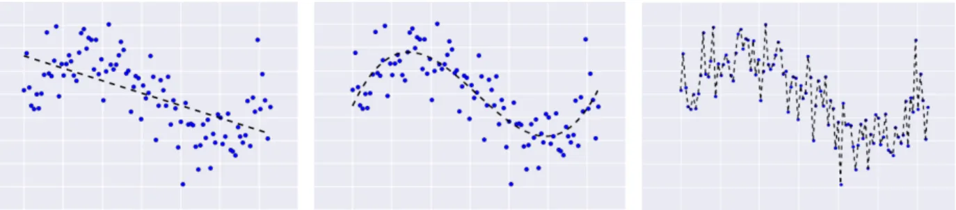
Figure 2.1. Increasingly complex models fit to sinusoidal data (EliteDataScience, 2018) What can go wrong when minimizing the training error ˆR as a surrogate for minimizing the true risk R? If the hypothesis class H allows for it, h can fit the data sample too closely, leading to a higher true risk than some hÕ that has a higher training error than h. More

precisely, h can be worse than hÕ even when ˆR(h) < ˆR(hÕ) because R(h) > R(hÕ). This can

be easily visualized by an example.

In Figure 2.1, we see data coming from a noisy sinusoid task (EliteDataScience, 2018). On the left, a linear model is fit to the data. This leads to both high training error and high true risk. In other words, the model is not complex enough. On the right, a much more complex model is fit to the data. This leads to zero training error, as the learned function fits every training point. However, it will also lead to high true risk as it will not generalize well to unseen data. This is because it is fitting the data too closely, fitting the noise in the data, and, hence, overfitting. The linear model was too simple at the highly complex model was too complex. In the middle, we see a model of about the right complexity that learns a function that will generalize the best of the three.

One notion of generalization that is often seen in statistical learning theory is the

gener-alization gap. This is simply the difference between the true risk and the training error:

Egap(h) = R(h) ≠ ˆR(h) (2.2.1)

2.3. Model Complexity

InFigure 2.1, the key concept that varies (increases from left to right) is model complexity (i.e., the complexity of the hypothesis class H). Models that are not sufficiently complex will underfit, while models that are too complex will overfit (see, e.g., Figure 2.1). In terms of hypothesis classes, the larger |H| is, the more functions exist that will fit the training data, but they might not perform well on unseen data. It is intuitive that the larger |H| is, the more our model will overfit (see Figure 3.1 in Section 3.2 for an illustration of this in the bias-variance framework). And indeed, there is theory that supports this intuition (Mohri

et al., 2012, Theorem 2.2). For any ” > 0, with probability at least 1 ≠ ”, ’h œ H, R(h) Æ ˆR(h) + Û log |H| + log2 ” 2m . (2.3.1)

The quantity |H| is one notion of model complexity. However, for many models (e.g. neural networks), |H| is infinite. Therefore, a better notion of model complexity is needed. The VC dimension of H, VC(H), is a better notion of model complexity, which leads to a finite bound with infinite models classes (Mohri et al., 2012, Chapter 3.3). For any ” > 0, with probability at least 1 ≠ ”,

’h œ H, R(h) Æ ˆR(h) + ˆ ı ı

Ù8VC(H) logVC(H)2em + 8 log4”

m . (2.3.2)

This bounds grows with VC(H). For many models the VC dimension ends up being roughly proportional to the number of parameters in the model. For example, the VC dimension of various kinds of neural networks grows with the number of parameters (Baum & Haussler,1989; Karpinski & Macintyre, 1995; Bartlett et al., 1998; Harvey et al., 2017).

Rademacher complexity is another measure of model complexity. Intuitively, it measures the capacity of a model to fit random noise. Generalization bounds in terms of Rademacher complexity are also prevalent (Mohri et al., 2012, Theorem 3.2):

’h œ H, R(h) Æ ˆR(h) + Rm(H) +

Û log 1

”

2m (2.3.3)

where Rm(H) denotes the Rademacher complexity of H. Known bounds on Rademacher

complexity also grow with the number of parameters (Bartlett & Mendelson, 2003).

These generalization bounds in terms of model complexity are important because of how they are interpreted. The general idea is that the model must be complex enough to achieve a low ˆR(h), but not too complex that the complexity measures such as VC(H) and Rm(H)

will blow up, leading to high bounds on R(h). For example, when interpreting the VC-based generalization bound, Abu-Mostafa et al. (2012, Chapter 2.2) wrote, “Although the bound is loose, it tends to be equally loose for different learning models, and hence is useful for comparing the generalization performance of these models. [...] In real applications, learning models with lower VC(H) tend to generalize better than those with higher VC(H). Because of this observation, the VC analysis proves useful in practice [...] the VC bound can be used as a guideline for generalization, relatively if not absolutely.”

Chapter 3

The Bias-Variance Tradeoff

3.1. What are Bias and Variance?

The bias is a measure of how close the central tendency of a learner is to the true function

f. If, on average (over training sets S), the learner learns the true function f, then the learner

is unbiased. For some x ≥ D, the bias is

Bias(hS) = ES[hS(x)] ≠ f(x) .

The variance is a measure of fluctuations of a learner around its central tendency, where the fluctuations result from different samplings of the training set. By definition, a learner that generalizes well does not learn dramatically different functions, depending on sampling of the training set. Let Y = R for simplicity; then for some x ≥ D, the variance is

Var(hS) = ES

Ë

(hS(x) ≠ ES[hS(x)])2

È

.

3.2. Intuition for the Tradeoff

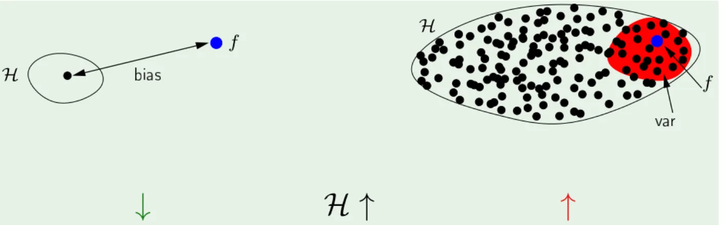
Similar to the idea that larger hypothesis classes lead to overfitting in Section 2.3, in the bias-variance context, there is the idea that larger hypothesis classes lead to higher variance. This is illustrated inFigure 3.1, which comes fromAbu-Mostafa et al.(2012). Also, illustrated is the idea that bias decreases when increasing the size of the hypothesis class because their will be more hypotheses that are closer to the true function f. In Figure 3.1, a hypothesis class that contains only a single hypothesis is depicted on the left; this will, of course, lead to bias as that hypothesis does not match f, but it will also lead to zero variance, which is a positive. In contrast, on the right, there is a larger hypothesis class (Figure 3.1); in this example, this leads to nearly zero bias, but it comes at the expense of incurring variance. The bottom of Figure 3.1 is shorthand that summarizes the idea that when you increase the size of the hypothesis class, you decreases bias and increase variance. Figure 2.1 is another example of this: the leftmost learner has high bias and low variance,

=

_E

¯

g(

x

)

f (

x

)

=

E

E

g

(

x

)

g(

¯

x

)

H

Figure 3.1. Bias-variance in simple vs. complex hypothesis class (Abu-Mostafa et al.,2012)

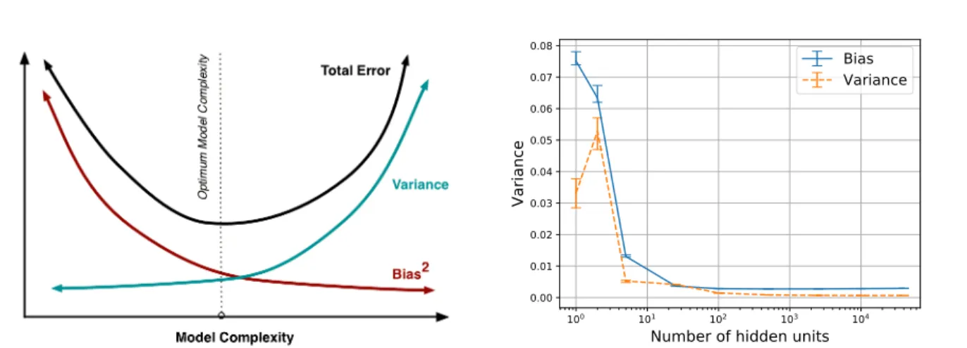
Figure 3.2. Illustration of the bias-variance tradeoff (Fortmann-Roe, 2012)

the rightmost learner has low bias and high variance, and the learner in the middle has something close to the optimal balance of bias and variance.

In their landmark paper, Geman et al. (1992) capture the essence of the bias-variance tradeoff with the following claim: “the price to pay for achieving low bias is high variance.” In Figure 3.2, we see the common illustration of the bias-variance tradeoff (Fortmann-Roe (2012)). Note the important U shape of the test error curve with increasing model complexity. The idea is that the optimal point on that U can be achieved by achieving the optimal balance of bias and variance. This tradeoff hypothesis is ubiquitious, as we will see in Section 3.4.2.

3.3. The Bias-Variance Decomposition

Geman et al. (1992) considered the average case (over training sets) quantity ESR(hS)

with squared-loss and showed that it can be cleanly decomposed into bias and variance 10

components:

ESR(hS) = Ebias(hS) + Evariance(hS) + Enoise (3.3.1)

Although a decomposition does not prove that the bias-variance tradeoff is true, it does show that the average error is made up of a sum of bias and variance components. Then, if the average error is held constant and bias is varied, variance must also vary (and vice versa). This greatly added to the strong intuition of the bias-variance tradeoff, and Geman et al. (1992) became quite highly cited for their contribution.

Note that risks computed with classification losses (e.g cross-entropy or 0-1 loss) do not have such a clean, additive bias-variance decomposition (Domingos, 2000; James, 2003). However, because the concept of a tradeoff is not reliant on an additive decomposition (see Hastie & Tibshirani(1990, Chapter 3.3) for presence of the bias-variance tradeoff before the bias-variance decomposition), the concept of the bias-variance tradeoff is applied extremely broadly (see Section 3.4.2), including settings where an additive decomposition does not seem possible.

3.4. Why do we believe the Bias-Variance Tradeoff?

A universal bias-variance tradeoff, without qualifications, is a mere hypothesis. Poten-tially, its most significant appeal comes from its intuitiveness. In this section, we review the history of the bias-variance tradeoff, the evidence in support of it, and its prevalence in textbooks (which also seem to contain much of the authoritative evidence).

3.4.1. A History

The concept that we know as the “bias-variance tradeoff” in machine learning has a long history, with its basis in statistics. Neural Networks and the Bias/Variance Dilemma (Geman et al., 1992) is the most cited work largely because it introduced the bias-variance decomposition to the machine learning community, provided convincing experiments with nonparametric methods, and popularized the bias-variance tradeoff in the neural network and machine learning community. However, the bias-variance tradeoff was already present in a textbook in 1990 (Hastie & Tibshirani,1990), and it dates back at least as far back as 1952 in statistics when Grenander (1952) referred to the concept as an “uncertainty principle.”

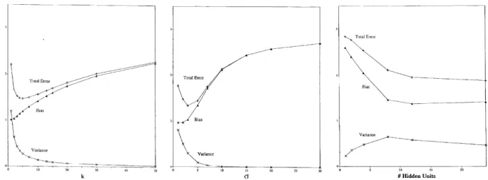
3.4.1.1. Experimental Evidence

Geman et al.(1992) ran experiments using two nonparametric methods (KNN and kernel regression) and neural networks on a partially corrupted version of the handwritten digits Guyon (1988) collected (Figure 3.3). The experiments on k-nearest neighbor (KNN) ( Fig-ure 3.3(a)) and kernel regression (Figure 3.3(b)) yield clear bias-variance tradeoff curves with

(a) K-nearest neighbor (KNN)

(higher k is less complexity) (b) Kernel regression (higher kernelwidth ‡ is less complexity) (c) Single hidden layer neural net-work (higher “# Hidden Units” is

more complexity)

Figure 3.3. Geman et al. (1992)’s bias-variance experiments on handwritten digits

U-shaped test error curves in their respective complexity parameters k and ‡. The exper-iment with neural networks (Figure 3.3(c)) is substantially less conclusive. Geman et al. (1992) maintain their claim that there is a bias-variance tradeoff in neural networks and explain their inconclusive experiments as a result of convergence issues:

«The basic trend is what we expect: bias falls and variance increases with

the number of hidden units. The effects are not perfectly demonstrated (no-tice, for example, the dip in variance in the experiments with the largest numbers of hidden units), presumably because the phenomenon of overfit-ting is complicated by convergence issues and perhaps also by our decision to stop the training prematurely. »

This is the first glimpse we see of the cracks in the bias-variance tradeoff hypothesis. There is a fair amount of empirical evidence for the bias-variance tradeoff in different complexity parameters in a variety of methods. Wahba & Wold (1975) show a tradeoff in complexity with cubic splines when varying their smoothing parameter. Geurts (2002, Section 5.4.3) show a bias-variance tradeoff in decision trees when varying tree size. Hastie & Tibshirani(1990, Chapter 3.3) show a bias-variance tradeoff with a “running-mean smoother” (i.e. KNN, but in statistics) when varying k. Bishop(2006, Chapter 3.2) show a bias-variance tradeoff with Gaussian basis function linear regression when varying the L2 regularization (weight decay) parameter ⁄. Goodfellow et al.(2016, Chapters 5.2 and 5.3) show a tradeoff in complexity with fitting polynomials when varying either the degree or the L2 regularization parameter.

3.4.1.2. Supporting Theory

The first main theory that supports the bias-variance tradeoff is the sample of general-ization upper bounds presented in Section 2.3 that grow with the number of parameters. This is simply because the bias-variance tradeoff is a clear conceptualization of one of the common interpretations of those bounds: models that are too simple will not perform well due to underfitting (high bias or high training error ˆR) while models that are too complex will not perform well due overfitting (high variance caused by high model complexity such as VC(H)). However, it should be noted that these upper bounds do not guarantee that a model with high VC(H) will actually have high variance (or high test error); a lower bound for cases seen in practice (not worst case) would be needed for that.

Hastie et al.(2001, Chapter 7.3) show that you can derive closed-form expressions for the variance for simple models such as KNN and linear regression in the “fixed-design” setting where the design matrix X is fixed. In this setting, Y = f(X)+‘, where f is the true function mapping examples x (rows in X) to y (elements in the vector Y ). Then, the randomness in Y is determined by the zero-mean random variable ‘. In this setting, Hastie et al. (2001, Chapter 7.3) show that variance for KNN models scales as 1

K. Similarly, they show that

the variance for linear regression grows linearly with the number of parameters, assuming

XT_X is invertible. Note that in the over-parameterized setting (XT_X is not invertible), we

show that the variance of linear regression does not grow with the number of parameters (see Section 5.5.1 inChapter 5).

Because neural networks are much more complicated models than KNN and linear regres-sion, we must resort to bounds on the variance of a neural network. Barron (1994) derives an upper bound on the estimation error of a single hidden layer neural network that grows linearly with the number of hidden units. The estimation error is not the same thing as variance, but it is analogous (see Section 3.5). This kind of bound is similar to the bounds described in Section 2.3. Again, it should be noted that because this is an upper bound, it does not actually imply that large neural networks will have high estimation error.

3.4.2. The Textbooks

The concept of the bias-variance tradeoff is ubiquitious, appearing in many of the text-books that are used in machine learning education: Hastie et al. (2001, Chapters 2.9 and 7.3), Bishop (2006, Chapter 3.2), Goodfellow et al. (2016, Chapter 5.4.4)), Abu-Mostafa et al. (2012, Chapter 2.3), James et al. (2014, Chapter 2.2.2), Hastie & Tibshirani (1990, Chapter 3.3), Duda et al. (2001, Chapter 9.3). Here are two excerpts:

— “As a general rule, as we use more flexible methods, the variance will increase and the bias will decrease. The relative rate of change of these two quantities determines whether the test MSE increases or decreases. As we increase the flexibility of a class

of methods, the bias tends to initially decrease faster than the variance increases. Consequently, the expected test MSE declines. However, at some point increasing flexibility has little impact on the bias but starts to significantly increase the variance. When this happens the test MSE increases” (James et al.,2014, Chapter 2.2.2). — “As the model complexity of our procedure is increased, the variance tends to increase

and the squared bias tends to decrease” (Hastie et al., 2001, Chapters 2.9).

3.5. Comparison to the Approximation-Estimation Tradeoff

The bias-variance tradeoff is not the only tradeoff in machine learning that is related to generalization. For example, when hS is chosen from a hypothesis class H, R(hS) can be

decomposed into approximation error and estimation error:

R(hS) = Eapp+ Eest

where Eapp = minhœHR(h) and Eest = R(hS) ≠ Eapp. Shalev-Shwartz & Ben-David (2014,

Section 5.2) present this decomposition and frame it as a tradeoff. Bottou & Bousquet(2008) describe this as the “well known tradeoff between approximation error and estimation error” and present it in a slightly more lucid way as a decomposition of the excess risk:

E[R(hS) ≠ R(hú)] = E[R(hú_H) ≠ R(hú)] + E[R(hS) ≠ R(hú_H)]

where R(hú) is the Bayes error and hú

H = arg minhœHR(h) is the best hypothesis in H. The

approximation error can then be interpreted as the distance of the best hypothesis in H from the Bayes classifier, and the estimation error can be interpreted as the average distance of the learned hypothesis from the best hypothesis in H. It is common to associate larger H with smaller approximation error and larger estimation error, just like it is common to associate larger H with smaller bias and larger variance. While bias (variance) and approximation error (estimation error) are qualitatively similar, they are not the exact same.

3.5.1. Universal Approximation Theorem for Neural Networks

The commonly cited universal approximation property of neural networks (Cybenko, 1989; Hornik, 1991; Leshno & Schocken, 1993) means that the approximation error goes to 0 as the network width increases; these results do not say anything about estimation error. In other words, the universal approximation error does not imply that wider networks are better. It implies that wider networks yield lower approximation error; traditional thinking suggests that this also means that wider networks yield higher estimation error.

Chapter 4

The Lack of a Tradeoff

4.1. A Refutation of Geman et al.’s Claims

In their highly influential paper, Geman et al. (1992) make several claims of varying specificity. We will start with their most general claim, which is simply a statement of the bias-variance tradeoff:

«the price to pay for achieving low bias is high variance. »

However, this claim is not true in the general case. The fact that the expected risk can be decomposed into squared bias and variance does imply that the two terms trade off. It is not necessary to trade bias for variance in all settings. For example, it is not necessary to trade bias for variance in neural networks (Neal et al. (2018),Chapter 5).

As neural networks are a main focus of Geman et al. (1992)’s work, they also make a clear claim relevant to neural networks: “bias falls and variance increases with the number of hidden units.” We directly test this claim in Chapter 5 and show it to be false on a variety of datasets. Both bias and variance can decrease as network width increases. In Figure 4.1we contrast the common intuition about the bias-variance tradeoff (left, as inspired by Figure 3.1) with what we observe in neural networks (right). This is a specific example of not having to pay any price of increased variance when decreasing bias.

In fact,Geman et al. (1992)’s own experiments with neural networks do not even support their claim that “bias falls and variance increases with the number of hidden units.” Geman et al. (1992, Figures 16 and 8) run experiments with a handwritten digit recognition dataset (Figure 4.2(a)) and with a sinusoid dataset (Figure 4.2(b)). In both of these datasets, they see decreasing variance when increasing the number of hidden units (Figure 4.2). Geman et al. (1992, page 33) explain this seeming evidence against their claim as a product of “convergence issues,” and maintain their claim: “The basic trend is what we expect: bias falls and variance increases with the number of hidden units. The effects are not perfectly demonstrated (notice, for example, the dip in variance in the experiments with the largest

unbiased biased with some variance bias high variance

Traditional view of bias-variance

increasing number of  parameters Practical setting low variance increasing network width

Worst-case analysis Measure concentrates

Figure 4.1. Bias-variance in simple vs. complex hypothesis class

numbers of hidden units), presumably because the phenomenon of overfitting is complicated by convergence issues and perhaps also by our decision to stop the training prematurely.”

In their paper,Geman et al.(1992) give the following prescription for choosing the width of a neural network: “How big a network should we employ? A small network, with say one hidden unit, is likely to be biased, since the repertoire of available functions spanned by f(x; w) over allowable weights will in this case be quite limited. If the true regression is poorly approximated within this class, there will necessarily be a substantial bias. On the other hand, if we overparameterize, via a large number of hidden units and associated weights, then the bias will be reduced (indeed, with enough weights and hidden units, the network will interpolate the data), but there is then the danger of a significant variance contribution to the mean-squared error.” Although this fits the conventional wisdom laid out in Section 2.3 and Chapter 3, we find this way of thinking to be misleading, leading researchers to incorrect predictions.

4.2. Similar Observations in Reinforcement Learning

Neyshabur et al. (2015) found that increasing the width of a single hidden layer neural network leads to decreasing test error on MNIST and CIFAR10 until it levels off (never going back up). We explore whether this phenomenon extends to deep reinforcement learning. We provide some evidence that it does, finding that wider networks do seem to perform better than their smaller counterparts in deep reinforcement learning as well (Neal & Mitliagkas, 2019). Combining that with the results from Chapter 5, we infer that very wide networks do not have to suffer from high variance (in exchange for low bias) in reinforcement learning either.

(a) Bias, variance, and total error as a function of number of hidden units in Geman et al. (1992)’s handwritten digit recognition experiment. Note that variance is decreasing with width in roughly the last 2

3 of the graph.

(b) Bias (o), variance (x), and total error (+) as a function of number of hidden units in Geman et al. (1992)’s noise-free (deterministic) and noisy (ambiguous) sinusoid classificia-tion experiments. Note that decreasing variance is already seen in the deterministic (top) experiment with neural net-works as small as 7-15 hidden units.

Figure 4.2. Geman et al. (1992)’s neural network experiments

4.3. Previous Work on Boosting

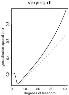
Bühlmann & Yu (2003)’s work on the bias-variance tradeoff in boosting is motivated by “boosting’s resistance to overfitting” when increasing the number of iterations. For example, in Schapire & Singer (1999, Figures 8-10), they run experiments on many datasets, finding that, on some datasets, test error decreases and plateaus without increasing with more iterations of boosting. This is only the case in some of their experiments, as in roughly half of their experiments, Schapire & Singer (1999) find that test error does eventually increase with number of iterations of boosting. Still, because roughly half of the experiments show “boosting’s resistance to overfitting,”Bühlmann & Yu(2003) study bias-variance in boosting. Bühlmann & Yu(2003) find that the lack of increasing test error when increasing number of iterations (“boosting’s resistance to overfitting”) can be explained in terms of bias and variance. In Theorem 1, they show exponentially decaying bias and variance that grows at an exponentially decaying rate with number of iterations. There are some specifics to this that are related to the strength/weakness of the learner that is boosted, but this is how they explain why monotonically decreasing test error can sometimes be seen when increasing the number of iterations in boosting: “(2) Provided that the learner is sufficiently weak, boosting always improves, as we show in Theorem 1” (Bühlmann & Yu,2003, Section 3.2.2).

boosting

m

generalization squared error

0 50 100 150 200 0.2 0.4 0.6 0.8 varying df degrees of freedom

generalization squared error

0 10 20 30 40

0.2

0.4

0.6

0.8

(a) Test error as a function of the number of iterations of boosting. Although it de-creases and then inde-creases, it inde-creases at a much slower rate than the classic bias-variance tradeoff would suggest (see figure on the right). Bühlmann & Yu (2003) call this slower increase an “a new exponential bias-variance tradeoff.”

boosting

m

generalization squared error

0 50 100 150 200 0.2 0.4 0.6 0.8 varying df degrees of freedom

generalization squared error

0 10 20 30 40

0.2

0.4

0.6

0.8

(b) Test error as a function of the amount of smoothing in a cubic spline. This is the test error curve that the classic bias-variance tradeoff would suggest; test error increases with the complexity parameter at a rate that is at least linear.

Figure 4.3. Exponential bias-variance tradeoff in boosting (Bühlmann & Yu, 2003) All this said,Bühlmann & Yu (2003)’s work should not be interpreted as showing a lack of a bias-variance tradeoff in boosting. Rather, it shows a bias-variance tradeoff where the growth of variance with the complexity parameter is exponentially smaller than that in the traditional bias-variance tradeoff (seeFigure 4.3), which implies that variance does not grow forever when increasing the number of iterations. Their work is an important example of a departure from the conventional bias-variance tradeoff.

4.4. The Double Descent Curve

A conjecture that has recently gained popularity is the idea the risk behaves as a “double descent” curve in model complexity (Figure 4.4). Specifically, the idea is that the risk behaves according to the classical bias-variance tradeoff wisdom (Chapter 3) in the under-parameterized regime; the risk decreases with model complexity in the over-under-parameterized

Ri

sk

Training risk

Test risk

Capacity of

_H

Ri

sk

Training risk

Test risk

Capacity of

_H

(a)

(b)

Figure 1: Curves for training risk (dashed line) and test risk (solid line). (a) The classical

U-shaped risk curve arising from the bias-variance trade-off. (b) The double descent risk curve,

which incorporates the U-shaped risk curve (i.e., the “classical” regime) together with the observed

behavior from using high capacity function classes (i.e., the “modern” interpolating regime),

sep-arated by the interpolation threshold. The predictors to the right of the interpolation threshold

have zero training risk.

When function class capacity is below the “interpolation threshold”, learned predictors exhibit

the classical U-shaped curve from Figure 1(a). (In this paper, function class capacity is identified

with the number of parameters needed to specify a function within the class.) The bottom of the

U is achieved at the sweet spot which balances the fit to the training data and the susceptibility

to over-fitting: to the left of the sweet spot, predictors are under-fit, and immediately to the

right, predictors are over-fit. When we increase the function class capacity high enough (e.g.,

by increasing the number of features or the size of the neural network architecture), the learned

predictors achieve (near) perfect fits to the training data—i.e., interpolation. Although the learned

predictors obtained at the interpolation threshold typically have high risk, we show that increasing

the function class capacity beyond this point leads to decreasing risk, typically going below the risk

achieved at the sweet spot in the “classical” regime.

All of the learned predictors to the right of the interpolation threshold fit the training data

perfectly and have zero empirical risk. So why should some—in particular, those from richer

functions classes—have lower test risk than others? The answer is that the capacity of the function

class does not necessarily reflect how well the predictor matches the inductive bias appropriate for

the problem at hand. For the learning problems we consider (a range of real-world datasets as well

as synthetic data), the inductive bias that seems appropriate is the regularity or smoothness of

a function as measured by a certain function space norm. Choosing the smoothest function that

perfectly fits observed data is a form of Occam’s razor: the simplest explanation compatible with

the observations should be preferred (cf. [38, 6]). By considering larger function classes, which

contain more candidate predictors compatible with the data, we are able to find interpolating

functions that have smaller norm and are thus “simpler”. Thus increasing function class capacity

improves performance of classifiers.

Related ideas have been considered in the context of margins theory [38, 2, 35], where a larger

function class

_{H may permit the discovery of a classifier with a larger margin. While the margins}

theory can be used to study classification, it does not apply to regression, and also does not

pre-dict the second descent beyond the interpolation threshold. Recently, there has been an emerging

recognition that certain interpolating predictors (not based on ERM) can indeed be provably

sta-tistically optimal or near-optimal [3, 5], which is compatible with our empirical observations in the

interpolating regime.

In the remainder of this article, we discuss empirical evidence for the double descent curve, the

3

Figure 4.4. Double descent curve, showing U-shaped risk curve in under-parameterized regime and decreasing curve in over-parameterized regime (Belkin et al., 2019a).

regime; and there is a sharp transition from the under-parameterized regime to the over-parameterized regime where the training error is 0. Belkin et al. (2019a) illustrate this in Figure 4.4.

In previous work, Advani & Saxe (2017) observed this phenomenon in linear student-teacher1 _{networks and with nonlinear networks on MNIST. In concurrent (to Chapter 5)}

work, Spigler et al. (2018); Geiger et al. (2019b); Belkin et al. (2019a) also studied this phenomenon. Spigler et al. (2018); Geiger et al. (2019b) described the cusp in the double descent curve as corresponding to a phase transition and draw the analogy to the “jamming transition” in particle systems. Belkin et al. (2019a) conjectured that this phenomenon is fairly general (as opposed to just being restricted to neural networks). Belkin et al. (2019a) showed the phenomenon in random forests, in addition to neural networks, and coined the term “double descent.” Nakkiran et al. (2019) recently showed that this double descent phenomenon is present in many state-of-the-art architectures such as convolutional neural networks, ResNets, and transformers, as opposed to only being present in more toy settings. The double descent phenomenon in simple settings such as shallow linear models can be seen in work that dates as far back as 1995 (Opper, 1995, 2001; Bös & Opper,1997).

Our work in Chapter 5 is consistent with the double descent curve. Although we were not looking for the cusp in the double descent curve (can require dense sampling of model sizes and specific experimental details), we do seem to see it in several variance figures in Chapter 5. All the works on the double descent curve examine the risk (or test error). In order to test the bias-variance hypothesis, it is important to actually measures bias and variance because test error and bias can decrease while variance still increases at an exponentially decaying rate (Section 4.3).

1. “Teacher” here refers to the fact that the data is generated by a neural network.

4.5. The Need to Qualify Claims about the Bias-Variance Tradeoff

when Teaching

Students who take introductory machine learning courses are typically taught the bias-variance tradeoff as a general, unavoidable truth that applies anywhere there is some notion of increasing model complexity (seeSection 3.4.2 for its prevalence and representative quotes from textbooks). This leads machine learning experts to sometimes make incorrect inferences about model selection with high confidence. From extensive personal communication, it appears that most researchers unfamiliar with work likeNeyshabur et al.(2015)’s react with incredulity to the results described in Section 4.1, Section 4.2, and Chapter 5. Even among researchers who have familiarized themselves with Neyshabur et al. (2015)’s results on test error, one can find many who are surprised by our results. We attribute this phenomenon to the strong influence Geman et al. (1992)’s claims have had on the research community. In other words, a sizable portion of researchers can be dogmatic about the conventional tradeoff wisdom described inSection 2.3andChapter 3. Qualifying the conventional tradeoff wisdom in textbooks and introductory courses by noting that the tradeoff intuition is useful sometimes and misleading other times would prevent future students from subscribing to this intuitive dogma.

The goal in amending textbooks/lectures that teach the bias-variance tradeoff is to make it more clear that the bias-variance tradeoff is not a universal truth. Here, we present three simple qualifications that, if integrated, would more accurately represent the evidence we have on the bias-variance tradeoff and would help prevent students from interpreting that the bias-variance tradeoff is universal:

(1) Expected error can be decomposed into (squared) bias and variance, when using squared loss (Geman et al., 1992), but this decomposition does not imply a tradeoff. This lack of implication should be made explicit in textbooks because the decomposition is often used in close proximity to the tradeoff as ambiguous evidence for it.

(2) The bias-variance tradeoff should not be assumed to be universal. There is evidence that bias and variance trade off in certain methods (e.g. KNN) when varying the right parameter (Section 3.4.1.1), but there are also counterexamples. For example, there are clear examples of a lack of a bias-variance tradeoff in neural networks (Chapter 5) and potentially other methods such as decision trees (Belkin et al., 2019a).

(3) It should be emphasized that the PAC upper bounds on test error can be very loose for the problems we care about in practice (see Sections 2.3 and 3.4.1.2 for examples of upper bounds on test error and estimation error). Because these upper bounds are so loose, their qualitative trend (e.g. as number of parameters increases)

is not necessarily an accurate reflection of the qualitative trend of the test error in practice.

Chapter 5

A Modern Take on the

Bias-Variance Tradeoff

in Neural Networks

by

Brady Neal1_{, Sarthak Mittal}1_{, Aristide Baratin}1_{, Vinayak Tantia}1_,

Matthew Scicluna1_{, Simon Lacoste-Julien}1_{, and Ioannis Mitliagkas}1

(1_{) Mila - Quebec AI Institute}

6666 St Urbain St, Montréal, QC H2S 3H1

This article was accepted at the ICML 2019 Workshop on Identifying and Understanding Deep Learning Phenomena.

The main contributions of Brady Neal for this articles are presented. — Lead the project

— Hypothesis that the bias-variance tradeoff would not be seen in neural networks when varying width

— The whole initial codebase — Ran many of the experiments — Proposition 5.5.1

— Majority of paper writing

Sarthak Mittal ran many experiments.

Vinayak Tantia contributed significantly to the codebase and ran experiments. Aristide Baratin contributed the initialization term to Proposition 5.5.1.

Aristide Baratin and Ioannis Mitliagkas proved related versions of Theorem 5.5.2

Ioannis Mitliagkas and Aristide Baratin contributed significantly to the writing of the paper.

Résumé. Le compromis biais-variance nous indique qu’à mesure que la complexité du modèle augmente, le biais diminue et la variance augmente, ce qui conduit à une courbe d’erreur de test en forme de U. Cependant, les résultats empiriques récents avec des réseaux neuronaux sur-paramétrés sont marqués par une absence frappante de la courbe d’erreur de test classique en forme de U : l’erreur de test continue de diminuer dans les réseaux plus larges. Cela donne à penser qu’il n’y a peut-être pas de compromis sur la variance de biais dans les réseaux de neurones en ce qui concerne la largeur du réseau, contrairement à ce que prétendaient, à l’origine, par exemple, Geman et al. (1992). Motivés par les preuves incertaines utilisées à l’appui de cette affirmation dans les réseaux de neurones, nous mesurons les biais et la variance dans le contexte moderne. Nous constatons que le biais d’accentuation et la variance peuvent diminuer à mesure que le nombre de paramètres augmente. Pour mieux comprendre cela, nous introduisons une nouvelle décomposition de la variance pour démêler les effets de l’optimisation et de l’échantillonnage des données. Nous fournissons également une analyse théorique dans un cadre simplifié qui est conforme à nos constatations empiriques.

Mots clés : compromis biais-variance, réseaux de neurones, sur-paramétrage, généralisation

Abstract.The bias-variance tradeoff tells us that as model complexity increases, bias falls and variances increases, leading to a U-shaped test error curve. However, recent empirical results with over-parameterized neural networks are marked by a striking absence of the classic U-shaped test error curve: test error keeps decreasing in wider networks. This suggests that there might not be a bias-variance tradeoff in neural networks with respect to network width, unlike was originally claimed by, e.g., Geman et al. (1992). Motivated by the shaky evidence used to support this claim in neural networks, we measure bias and variance in the modern setting. We find that both bias and variance can decrease as the number of parameters grows. To better understand this, we introduce a new decomposition of the variance to disentangle the effects of optimization and data sampling. We also provide theoretical analysis in a simplified setting that is consistent with our empirical findings. Keywords: bias-variance tradeoff, neural networks, over-parameterization, generalization

5.1. Introduction

There is a dominant dogma in machine learning: 24

«The price to pay for achieving low bias is high variance (Geman et al., 1992). »

The quantities of interest here are the bias and variance of a learned model’s prediction on a new input, where the randomness comes from the sampling of the training data. This idea that bias decreases while variance increases with model capacity, leading to a U-shaped test error curve is commonly known as the bias-variance tradeoff (Figure 5.1 (left)).

There exist experimental evidence and theory that support the idea of a tradeoff. In their landmark paper, Geman et al. (1992) measure bias and variance in various models. They show convincing experimental evidence for the bias-variance tradeoff in nonparametric meth-ods such as kNN (k-nearest neighbor) and kernel regression. They also show experiments on neural networks and claim that bias decreases and variance increases with network width. Statistical learning theory (Vapnik, 1998) successfully predicts these U-shaped test error curves implied by a tradeoff for a number of classic machine learning models. A key element is identifying a notion of model capacity, understood as the main parameter controlling this tradeoff.

Surprisingly, there is a growing amount of empirical evidence that wider networks gener-alize better than their smaller counterparts (Neyshabur et al.,2015;Zagoruyko & Komodakis, 2016; Novak et al., 2018; Lee et al., 2018; Belkin et al., 2019a; Spigler et al., 2018; Liang et al.,2017;Canziani et al.,2016). In those cases the classic U-shaped test error curve is not observed.

A number of different research directions have spawned in response to these findings. Neyshabur et al. (2015) hypothesize the existence of an implicit regularization mechanism. Some study the role that optimization plays (Soudry et al., 2018; Gunasekar et al., 2018). Others suggest new measures of capacity (Liang et al., 2017; Neyshabur et al., 2019). All approaches focus on test error, rather than studying bias and variance directly (Neyshabur et al., 2019; Geiger et al., 2019a; Liang et al.,2017;Belkin et al., 2019a).

Test error analysis does not give a definitive answer on the lack of a bias-variance tradeoff. Consider boosting: it is known that its test error often decreases with the number of rounds (Schapire & Singer,1999, Figures 8-10). In spite of this monotonicity in test error,Bühlmann & Yu (2003) show that variance grows at an exponentially decaying rate, calling this an “exponential bias-variance tradeoff” (see Section 4.3). To study the bias-variance tradeoff, one has to isolate and measure bias and variance individually. To the best of our knowledge, there has not been published work reporting such measurements on neural networks since Geman et al.(1992).

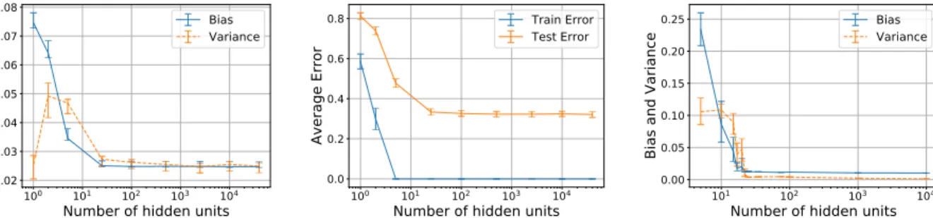
We go back to basics and study bias and variance. We start by taking a closer look at Geman et al. (1992, Figure 16 and Figure 8 (top))’s experiments with neural networks. We notice that their experiments do not support their claim that “bias falls and variance increases with the number of hidden units.” The authors attribute this inconsistency to convergence

Figure 5.1. On the left is an illustration of the common intuition for the bias-variance tradeoff (Fortmann-Roe, 2012). We find that both bias and variance decrease when we increase network width on MNIST (right) and other datasets (Section 5.4). These results seem to contradict the traditional intuition of a strict tradeoff.

issues and maintain their claim that the bias-variance tradeoff is universal. Motivated by this inconsistency, we perform a set of bias-variance experiments with modern neural networks.

We measure prediction bias and variance of fully connected neural networks. These measurements allow us to reason directly about whether there exists a tradeoff with respect to network width. We find evidence that both bias and variance can decrease at the same time as network width increases in common classification and regression settings (Figure 5.1 and Section 5.4).

We observe the qualitative lack of a bias-variance tradeoff in network width with a num-ber of gradient-based optimizers. In order to take a closer look at the roles of optimization and data sampling, we propose a simple decomposition of total prediction variance ( Sec-tion 5.3.3). We use the law of total variance to get a term that corresponds to average (over data samplings) variance due to optimization and a term that corresponds to variance due to training set sampling of an ensemble of differently initialized networks. Variance due to opti-mization is significant in the under-parameterized regime and monotonically decreases with width in the over-parameterized regime. There, total variance is much lower and dominated by variance due to sampling (Figure 5.2).

We provide theoretical analysis, consistent with our empirical findings, in simplified anal-ysis settings: i) prediction variance does not grow arbitrarily with number of parameters in fixed-design linear models; ii) variance due to optimization diminishes with number of pa-rameters in neural networks under strong assumptions.

Organization. The rest of this paper is organized as follows. We discuss relevant related work in Section 5.2. Section 5.3 establishes necessary preliminaries, including our variance

Figure 5.2. Trends of variance due to sampling and variance due to optimization with width on CIFAR10 (left) and on SVHN (right). Variance due to optimization decreases with width, once in the over-parameterized setting. Variance due to sampling plateaus and remains constant. This is in contrast with what the bias-variance tradeoff would suggest. decomposition. InSection 5.4, we empirically study the impact of network width on variance. In Section 5.5, we present theoretical analysis in support of our findings.

5.2. Related work

Neyshabur et al. (2015); Neyshabur (2017) point out that because increasing network width does not lead to a U-shaped test error curve, there must be some form of implicit regularization controlling capacity. Our work is consistent with this finding, but by ap-proaching the problem from the bias-variance perspective, we gain additional insights: 1) We specifically address the hypothesis that decreased bias must come at the expense of in-creased variance (seeGeman et al.(1992) andAppendix E) by measuring both quantities. 2) Our more fine-grain approach reveals that variance due to optimization vanishes with width, while variances due to sampling increases and levels off. This insight about variance due to sampling is consistent with existing variance results for boosting (Bühlmann & Yu, 2003). To ensure that we are studying networks of increasing capacity, one of the experimental controls we use throughout the paper is to verify that bias is decreasing.

In independent concurrent work, Spigler et al. (2018); Belkin et al. (2019a) point out that generalization error acts according to conventional wisdom in the under-parameterized setting, that it decreases with capacity in the over-parameterized setting, and that there is a sharp transition between the two settings. Although the phrase “bias-variance trade-off” appears in Belkin et al. (2019a)’s title, their work really focuses on the shape of the test error curve: they argue it is not the simple U-shaped curve that conventional wisdom would suggest, and it is not the decreasing curve that Neyshabur et al. (2015) found; it is “double descent curve,” which is essentially a concatenation of the two curves. This is in contrast