HAL Id: hal-00416446
https://hal.archives-ouvertes.fr/hal-00416446
Submitted on 15 Sep 2009
HAL is a multi-disciplinary open access
archive for the deposit and dissemination of sci-entific research documents, whether they are pub-lished or not. The documents may come from teaching and research institutions in France or abroad, or from public or private research centers.
L’archive ouverte pluridisciplinaire HAL, est destinée au dépôt et à la diffusion de documents scientifiques de niveau recherche, publiés ou non, émanant des établissements d’enseignement et de recherche français ou étrangers, des laboratoires publics ou privés.
Efficient Tools for Computing the Number of
Breakpoints and the Number of Adjacencies between
two Genomes with Duplicate Genes
Sébastien Angibaud, Guillaume Fertin, Irena Rusu, Annelyse Thevenin,
Stéphane Vialette
To cite this version:
Sébastien Angibaud, Guillaume Fertin, Irena Rusu, Annelyse Thevenin, Stéphane Vialette. Efficient Tools for Computing the Number of Breakpoints and the Number of Adjacencies between two Genomes with Duplicate Genes. Journal of Computational Biology, Mary Ann Liebert, 2008, 15 (8), pp.1093-1115. �10.1089/cmb.2008.0061�. �hal-00416446�
Efficient Tools for Computing the Number of
Breakpoints and the Number of Adjacencies between
two Genomes with Duplicate Genes
S´ebastien Angibaud
∗Guillaume Fertin
†Irena Rusu
‡Annelyse Th´evenin
§St´ephane Vialette
¶March 19, 2008
Abstract
Comparing genomes of different species is a fundamental problem in comparative genomics. Recent research has resulted in the introduction of different measures be-tween pairs of genomes: reversal distance, number of breakpoints, number of common or conserved intervals, etc. However, classical methods used for computing such mea-sures are seriously compromised when genomes have several copies of the same gene ∗Laboratoire d’Informatique de Nantes-Atlantique (LINA), UMR CNRS 6241, Universit´e de Nantes,
2 rue de la Houssini`ere, 44322 Nantes Cedex 3, France, Sebastien.Angibaud@univ-nantes.fr, Phone: (+33) 2 51 12 59 68, Fax: (+33) 2 51 12 58 12
†Laboratoire d’Informatique de Nantes-Atlantique (LINA), UMR CNRS 6241, Universit´e de Nantes,
2 rue de la Houssini`ere, 44322 Nantes Cedex 3, France, Guillaume.Fertin@univ-nantes.fr, Phone: (+33) 2 51 12 58 14, Fax: (+33) 2 51 12 58 12
‡Laboratoire d’Informatique de Nantes-Atlantique (LINA), UMR CNRS 6241, Universit´e de Nantes, 2 rue
de la Houssini`ere, 44322 Nantes Cedex 3, France, Irena.Rusu@univ-nantes.fr, Phone: (+33) 2 51 12 58 16, Fax: (+33) 2 51 12 58 12
§Laboratoire de Recherche en Informatique (LRI), UMR CNRS 8623, Universit´e Paris-Sud, 91405 Orsay,
France, thevenin@lri.fr, Phone: (+33) 1 69 15 70 99, Fax: (+33) 1 69 15 65 86.
¶IGM-LabInfo, UMR CNRS 8049, Universit´e Paris-Est, 5 Bd Descartes 77454 Marne-la-Vall´ee, France,
scattered across them. Most approaches to overcome this difficulty are based either on the exemplar model, which keeps exactly one copy in each genome of each duplicated gene, or on the maximum matching model, which keeps as many copies as possible of each duplicated gene. The goal is to find an exemplar matching, respectively a maximum matching, that optimizes the studied measure. Unfortunately, it turns out that, in presence of duplications, this problem for each above-mentioned measure is NP-hard.
In this paper, we propose to compute the minimum number of breakpoints and the maximum number of adjacencies between two genomes in presence of duplications us-ing two different approaches. The first one is a (exact) generic 0–1 linear programmus-ing approach, while the second is a collection of three heuristics. Each of these approaches is applied on each problem and for each of the following models: exemplar, maximum matching and intermediate model, that we introduce here. All these programs are run on a well-known public benchmark dataset of γ-Proteobacteria, and their performances are discussed.
Keywords: genome rearrangements, number of breakpoints, number of adjacen-cies, exemplar/matching/intermediate models, 0–1 linear programming
1
Introduction
It is a well-known fact that, between different species, the order of genes in the genomes is not conserved. Hence, it appears natural to exploit this information, in order for instance to infer the phylogenetic relationships between those species. Comparison of gene orders is usually done between pairs of genomes, and can be undertaken in many different ways, which fall into two main categories. The first one consists in defining different types of rearrangement operations, and to find a most parsimonious rearrangement scenario that, using these operations, allows to go from one genome to the other. Probably the most famous example is the reversal distance problem, in which only one operation, reversal, is allowed (see for instance (Hannenhalli and Pevzner, 1999)). The second category consists in computing a (dis-)similarity measure between two genomes, that is a number which reflects the proximity (or not) of the two considered genomes. In that case, the measure is computed regardless of any possible rearrangement scenario that would lead from one genome to the other. Several (dis-)similarity measures between two whole genomes have been proposed in the past: number of breakpoints (Watterson et al., 1982), number of common intervals (Uno and Yagiura, 2000), number of conserved intervals (Bergeron and Stoye, 2003), Maximum Adjacency Disruption (MAD) number (Sankoff and Haque, 2005).
In this paper, we will only be interested in the latter category. Moreover, our study focuses on genomes where genes possibly have several copies. When such duplications are present, in order to compute any measure between two genomes, one first needs to disambiguate the data by inferring orthologs, i.e., a non-ambiguous one-to-one mapping between the genes of the two genomes. In order to achieve this, two approaches have been considered recently: the exemplar model and the maximum matching model. In the exemplar model (Sankoff, 1999),
for all gene families, all but one occurrence in each genome are deleted. In the maximum matching model (Blin et al., 2004), the goal is to map as many genes as possible. These two models can be considered as the extremal cases of the same generic homolog assignment approach.
Unfortunately, it has been shown that, for each of the above mentioned measures, and for each model (exemplar or maximum matching), the problem of finding the non-ambiguous one-to-one mapping that optimizes the studied (dis-)similarity measure becomes NP-hard as soon as duplicates are present in genomes (Bryant, 2000; Blin et al., 2004; Blin and Rizzi, 2005; Blin et al., 2007) ; several inapproximability results are known (Thach, 2005; Chen et al., 2006b; Chen et al., 2006a; Blin et al., 2007; Angibaud et al., 2008), and in some cases, heuristic (hence, not exact) methods have been devised to obtain good solutions in a reasonable amount of time (Blin et al., 2005; Bourque et al., 2005; Angibaud et al., 2007b). The main goal of this paper is to study two measures, the number of breakpoints and the number of adjacencies, under three different models: the exemplar model, the maximum matching model and a model we introduce here, the intermediate model, in which, for all gene families, at least one occurrence in each genome is kept. In other words, in this model, one is allowed to modulate the number of conserved copies of each duplicated gene in each genome. Indeed, it seems natural to take this new model into account, because it is a generalization of both the exemplar and maximum matching models. We will actually discuss the interest of the intermediate model later in the paper, according to the results that will be presented. We will then focus on methods to answer the problems: given two genomes, find the exemplar (respectively intermediate, maximum) matching that maximizes the number of adjacencies (or minimizes the number of breakpoints). Extending research initiated in
(An-gibaud et al., 2007b), we propose, for each problem, a generic 0–1 linear programming method that exactly (though not always quickly) answers the question. We then provide, for each problem, several heuristics and compare them with results obtained by 0–1 linear programming on a dataset of γ-Proteobacteria. In addition, we show strong evidence that our fast and simple heuristics based on iteratively finding Longest Common Subsequences provide very good results on our dataset.
The paper is organized as follows. In Section 2, we present some preliminaries and definitions. In Section 3, we reduce our study, that we wish to perform for two measures and three models, to only three main problems. In Section 4, for each of these three problems, we provide the corresponding 0–1 linear programming encoding, together with some reduction rules that help speed-up the computation. In Section 5, we present and discuss the results that we have obtained by running our 0–1 linear programming methods on a dataset of γ-Proteobacteria. In Section 6, a collection of three heuristics is proposed and their results are compared to the exact results obtained in Section 5.
2
Preliminaries
From an algorithmic perspective, a unichromosomal genome is a signed sequence over a finite alphabet, referred hereafter as the alphabet of gene families. Each element of the sequence is called a gene. DNA has two strands, and genes on a genome have an orientation that reflects the strand on which the genes lie. We represent the order and orientation of the genes on each genome as a sequence of signed genes, i.e., genes with a sign, “+” or “−”. Let G1 and
G2 be two genomes, and let nx, x ∈ {1, 2} be the number of genes in genome Gx. For each
x ∈ {1, 2}, Gx[i] denotes the gene at position i (1 ≤ i ≤ nx) in Gx, and occx(g, i, j) denotes
the number of genes g (and −g) in Gx between positions i and j, 1 ≤ i ≤ j ≤ nx. To
simplify notations, we abbreviate occx(g, 1, nx) to occx(g). As we shall only be concerned
here with pairs of genomes (G1, G2) having the same gene content, we shall ignore those
genes that occur in one genome but not in the other.
In order to deal with the inherent ambiguity of duplicate genes, we now precisely define what is a matching between two genomes. Roughly speaking, a matching between two genomes can be seen as a way to describe a putative assignment of orthologous pairs of genes between the two genomes (see for example (Chen et al., 2005)). More formally, a matching M between genomes G1 and G2 is a set of pairwise disjoint pairs (G1[i], G2[j]), where G1[i]
and G2[j] belong to the same gene family regardless of the sign, i.e., |G1[i]| = |G2[j]|. Genes
of G1 and G2 that belong to a pair of the matching M are said to be saturated by M, or
M-saturated for short. The size of a matching M is noted by |M|. A matching M between G1 and G2 is said to be maximum if for any gene family, there are no two genes of this family
that are unmatched for M and belong to G1 and G2, respectively.
between two genomes. Two types of matchings are usually considered and specify the un-derlying model to focus on for computing the desired measure. In the exemplar model, the matching M is required to saturate exactly one gene of each gene family ; thus, the size of the matching is the number of gene families. In the maximum matching model, the matching M is required to be maximum, i.e., to saturate as many genes of any gene family as possible. Here again, the size of M can be easily computed in advance, from the two input genomes. In this paper, we present and study a third model, that we call the intermediate model. In this model, the matching M is required to saturate at least one gene of each gene family. In that sense, this new model lies between the two extrema that are the exemplar and the maximum matching models.
Let M be any matching between G1and G2that fulfills the requirements of a given model
(exemplar, intermediate or maximum matching). By first deleting non-saturated genes and next renaming genes in G1 and G2 according to the matching M, we may now assume that
both G1 and G2 are duplication-free, i.e. G2 is a signed permutation of G1. We call the
resulting genomes M-pruned.
Let G1 and G2 be two duplication-free genomes of size n. Without loss of generality,
we may assume that G1 is the identity positive permutation, i.e., G1 = +1 + 2 . . . + n.
We say that there is a breakpoint after gene G1[i], 1 ≤ i < n − 1, in G1 if neither G1[i]
and G1[i + 1] nor −G1[i + 1] and −G1[i] are consecutive genes in G2, otherwise we say that
there is an adjacency after gene G1[i]. In order to take into account the breakpoints and/or
adjacencies that arise at the extremities of the genomes, we artificially add, for each genome in the studied pair, a unique (i.e., non-duplicated) gene at both extremities. For simplicity, the artificial gene added before the first gene in both genomes will always be +0, while the
one added after the last gene will always be +(n + 1).
For example, if G1 = +1 + 2 + 3 + 4 + 5 + 6 and G2 = +1 −6 −5 −4 + 3 + 2,
we modify both genomes in order to obtain: G′
1 = +0 + 1 + 2 + 3 + 4 + 5 + 6 + 7 and
G′
2 = +0 + 1 −6 −5 −4 + 3 + 2 + 7. In this example, we have breakpoints in G′1 after
genes 1, 2, 3 and 6 and hence we have adjacencies in G′
1 after genes 0, 4 and 5. Thus, the
number of breakpoints between G1 and G2 is equal to 4, while the number of adjacencies
3
The problems
Given two genomes G1 and G2 and a model (exemplar, intermediate or maximum matching),
we wish to find a matching which (1) is appropriate to the model, and (2) yields the optimal number of breakpoints/adjacencies, where optimal means minimum for breakpoints and maximum for adjacencies. Not all of the six resulting problems are essentially different. In fact, only three of them are.
3.1
From six problems to four
Let G1 and G2 be two genomes and M be a matching between G1 and G2 under any model
(exemplar, intermediate or maximum matching). We define bkp(M) to be the number of breakpoints between the two M-pruned genomes. The number of adjacencies between two M-pruned genomes is denoted by adj(M).
It is easy to see, but important to notice, that for any matching M between two genomes G1 and G2, we have
adj(M) + bkp(M) = |M| + 1. (1)
Hence, for any given instance, if the size of the matching M is fixed, then finding the matching which minimizes the number of breakpoints is equivalent to finding the matching that maximizes the number of adjacencies, because of equality (1). As a consequence, we have the following proposition.
Proposition 1 Minimizing the number of breakpoints under the exemplar model is equiv-alent to maximizing the number of adjacencies ; the same result holds for the maximum
matching model.
For the intermediate model, the same result does not hold anymore, since the cardinality of the matching cannot be inferred from the input.
3.2
From four problems to three
Another, less straightforward, equivalence holds between two of our remaining problems.
Proposition 2 Minimizing the number of breakpoints under the exemplar model is equiva-lent to minimizing the number of breakpoints under the intermediate model.
Proof. Let G1 and G2 be two genomes. Denote by bkpoptE and bkp opt
I the minimum
num-ber of breakpoints obtained for G1 and G2 under the exemplar and intermediate models,
respectively.
Obviously, we have bkpoptE ≥ bkpoptI since any solution for the exemplar model is also a solution for the intermediate problem. What is left is thus to prove bkpoptE ≤ bkpoptI .
To this end, consider an optimal solution of the problem for the intermediate model, that is, a matching between genes of G1 and G2 yielding bkpoptI breakpoints. We then
construct a solution (G′
1, G′2) for the exemplar model that has at most bkp opt
I breakpoints.
This is done using the following greedy algorithm: while there exists two saturated genes in G1 that belong to the same gene family (regardless of the sign), delete one of the two
genes arbitrarily, together with the corresponding gene in G2. The above algorithm certainly
results in a solution for the exemplar model. We claim that this solution has at most as many breakpoints as the solution for the intermediate model, that is bkpoptI . To this aim, we consider any iteration of the above algorithm and show that the obtained matching has
at most as many breakpoints as the initial one. Four cases need distinct examination. For all genes a, the notation aN denote the presence of a breakpoint after the gene a.
1. G1 = . . . a X b . . ., G2 = . . . a X b . . . or G2 = . . . −b −X −a . . .
Deleting X in both genomes results in genomes G′
1 = . . . a b . . ., G′2 = . . . a b . . . or
G′2 = . . . −b −a . . . where no additional breakpoint is introduced.
2. G1 = . . . aNX b . . ., G2 = . . . c X b . . . or G2 = . . . −b −X c . . .
Deleting X in both genomes results in genomes G′
1 = . . . aNb . . ., G
′
2 = . . . c b . . . or
G′
2 = . . . −b c . . . where no additional breakpoint is introduced.
3. G1 = . . . a XNb . . ., G2 = . . . c X b . . . or G2 = . . . b −X −c . . .
Deleting X in both genomes results in genomes G′
1 = . . . aNb . . ., G
′
2 = . . . c b . . . or
G′2 = . . . b −c . . . where no additional breakpoint is introduced.
4. G1 = . . . aNXNb . . .
For any arbitrary G2, deleting X in both genomes induces either genome G′1 = . . . a b . . .
or genome G′
1 = . . . aNb . . .. In both cases, the number of breakpoints strictly decreases,
which contradicts the optimality of the solution under the intermediate model. There-fore, this case cannot happen.
For each case, deleting X in both genomes induces two genomes where no additional breakpoint is introduced. Therefore, the generated solution cannot admit more breakpoints than bkpoptI , and hence we have bkpoptI = bkpoptE . ✷
3.3
The three main problems
We are now in position to formally define the optimization problems we are interested in. As before, G1 and G2 are two genomes.
Let optE (respectively optM) be the problem of finding an exemplar (respectively
max-imum) matching M such that the corresponding M-pruned of G1 and G2 has a maximum
number of adjacencies. Proposition 1 insures that the same matching M also minimizes, after M-pruning G1 and G2, the number of breakpoints. We denote by adjoptE and bkp
opt E
(resp. adjoptM and bkpoptM ) the number of adjacencies and the number of breakpoints in an optimal solution to optE (resp. optM).
Let optIA (respectively optIB) be the problem of finding an intermediate matching M such that the corresponding M-pruned of G1 and G2 has a maximum number of adjacencies
(minimum number of breakpoints, respectively).
According to Proposition 2, as long as we are mainly interested in minimizing the number of breakpoints, we do not need to specifically solve optIB, assuming we solve optE. We denote by adjoptI and bkpoptI adjoptI and bkpoptI are the number of adjacencies and the number of breakpoints in an optimal solution to optIA and optIB, respectively.
4
An exact 0–1 linear programming approach
4.1
Introduction
Minimizing the number of breakpoints between two genomes with duplicated genes is an NP-hard problem for the exemplar model, even when occ1(g) = 1 for all genes g in G1
and occ2(g) ≤ 2 for all genes g in G2 (Bryant, 2000). Consequently, the NP-hardness
also holds for both the intermediate and the maximum matching models, which means that problems optE (and thus optIB, see Proposition 2) and optM are NP-hard. Moreover, a
recent result (Chen et al., 2007) implies that optIA is NP-hard as well.
Aiming at precise evaluations of heuristics, we develop in this section an exact generic approach as initiated in (Angibaud et al., 2007a). More precisely, our approach relies on expressing the different problems as 0–1 linear programs (Schrijver, 1998) and using powerful solvers to obtain optimal solutions.
For ease of exposition, we first present the complete 0–1 linear program for maximizing the number of adjacencies for the maximum matching problem (problem optM). Next we give some data reduction rules for reducing the input size, and hence speeding-up the program. Finally, we show how to adapt this program to optE and optIA.
4.2
Maximizing the number of adjacencies under the maximum
matching model: Problem opt
MThe 0–1 linear program we propose here (referred in the sequel to as Program Adjacency--Maximum-Matching) takes as input two genomes with duplicated genes, and solves problem optM. We denote by G the set of all gene families. The program is presented in Figure 1. How
to adapt the program for dealing with other problems of interest is deferred to Subsection 4.4.
Here, Figure 1
Program Adjacency-Maximum-Matching considers two genomes G1 and G2 of respective
lengths n1 and n2. The objective function, the variables and the constraints involved are
now discussed. Variables:
• Variables a(i, k), 1 ≤ i ≤ n1 and 1 ≤ k ≤ n2, define a matching M: ai,k = 1 iff G1[i]
is matched with G2[k] in M.
• Variables bx(i), x ∈ {1, 2} and 1 ≤ i ≤ nx, represent the M-saturated genes: bx(i) =
1 if and only if Gx[i] is saturated by the matching M. Clearly,
P
1≤i≤n1b1(i) =
P
1≤k≤n2b2(k), and this is precisely the size of M.
• Variables cx(i, j), x ∈ {1, 2} and 1 ≤ i < j ≤ nx, represent consecutive genes according
to M: cx(i, j) = 1 iff Gx[i] and Gx[j] are both saturated by M and no gene Gx[p],
i < p < j, is saturated by M.
• Variables d(i, j, k, ℓ), 1 ≤ i < j ≤ n1 and 1 ≤ k < ℓ ≤ n2, represent adjacencies
according to M: d(i, j, k, ℓ) = 1 iff
– either (G1[i], G2[k]) and (G1[j], G2[ℓ]) belong to M, G1[i] = G2[k] and G1[j] =
G2[ℓ], or (G1[i], G2[ℓ]) and (G1[j], G2[k]), and belong to M, G1[i] = −G2[ℓ] and
– G1[i] and G1[j] are consecutive in G1 according to M, and
– G2[k] and G2[ℓ] are consecutive in G2 according to M.
Constraints:
Assume x ∈ {1, 2}, 1 ≤ i < j ≤ n1 and 1 ≤ k < ℓ ≤ n2.
• Constraint C.01 ensures that each gene of G1 and of G2 is matched at most once,
i.e., b1(i) = 1 (respectively b2(k) = 1) iff gene i (respectively k) is matched in G1
(respectively G2) ; see Figure 2 for an illustration of this constraint. Observe that in
any matching, any two genes that are mapped together necessarily belong to the same gene family, and hence we do not have to explicitly ask for a(i, k) = 0 in case G1[i]
and G2[k] are two genes belonging to different gene families.
• Constraint C.02 actually defines the considered model (here the maximum matching model). For each gene family g, min(occ1(g), occ2(g)) occurrences of genes belonging
to g must be M-saturated in both G1 and G2 (see Figure 2).
• Constraints in C.03 and C.04 are concerned with our definition of consecutive genes. Variable cx(i, j) is equal to 1 iff there exists no p such that i < p < j and bx(p) = 1. It
is worth noticing here that, according to these constraints, one may have cx(i, j) = 1
even if one of the genes Gx[i] or Gx[j] is not M-saturated.
• Constraints in C.05 to C.10 define variables d. In the case where G1[i] = G2[k] and
G1[j] = G2[ℓ], Constraints C.05 and C.06 ensure that we have d(i, j, k, ℓ) = 1 if and
only if all variables a(i, k), a(j, ℓ), c1(i, j) and c2(k, ℓ) are equal to 1. In the case
we have d(i, j, k, ℓ) = 1 iff all variables a(i, ℓ), a(j, k), c1(i, j) and c2(k, ℓ) are equal to
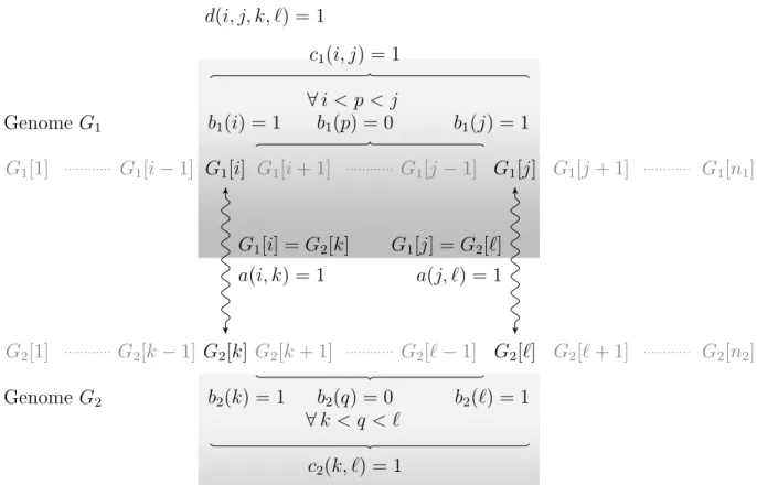
1. Constraint C.09 sets variable d(i, j, k, ℓ) to 0 if none of the two above cases holds. Finally, thanks to Constraint C.10, one must have at most one adjacency for every pair (i, j). See Figure 3 for a simple illustration.
The objective of Program Adjacency-Maximum-Matching is to maximize the number of adjacencies between the two considered genomes. According to the above, this objective thus reduces in our model to maximizing the sum of all variables d(i, j, k, ℓ).
Here, Figure 2
Here, Figure 3
4.3
Speeding-up the program
Program Adjacency-Maximum-Matching has O((n1· n2)2) variables and O((n1· n2)2)
con-straints. Aiming at speeding-up the execution of the program, we present here some simple rules for reducing the number of variables and constraints involved.
Pre-processing the genomes. The genomes are pairwise pre-processed to delete all genes that do not appear in both genomes. For instance, for the γ-Proteobacteria benchmark set studied in Section 5, the average size of a genome reduces from 3000 to 1300.
Reducing the number of variables and constraints. For non-duplicated genes, i.e., genes g for which occ1(g) = occ2(g) = 1, the corresponding variable ai,k is set directly to
1, as well as the two variables b1(i) and b2(k). Also, if two non-duplicated genes occur
consecutively or in reverse order with opposite signs, the corresponding variable d is set directly to 1 and the related constraints are discarded. If for two genes, say occurring at positions i and j in G1, at least one gene occurring between position i and j in G1 must
be saturated in any matching M (for example if one family has all occurrences between i and j in G1), then the corresponding variable c1(i, j) and the variable d(i, j, k, ℓ) for all
1 ≤ k < ℓ ≤ n2 are set directly to 0 and the related constraints are discarded. We can use
the same reasoning for two positions k and ℓ in G2 and the variables c2(k, ℓ) and d(i, j, k, ℓ)
for all 1 ≤ i < j ≤ n1.
4.4
Dealing with other measures and models
Program Adjacency-Maximum-Matching allows us to solve problem optM. We describe here how to adapt this 0–1 linear program for dealing with the two remaining problems, namely optE and optIA. As we shall see, only a few modifications are needed.
Exemplar Model (Problem optE). As observed before, Constraint C.02 explicits the
model under consideration. For the exemplar model, exactly one occurrence in each gene family must be saturated. Therefore, Constraint C.02 should be rewritten as follows.
C.02 ∀ x ∈ {1, 2}, ∀ g ∈ G, X
1≤i≤nx
|Gx[i]|=|g|
Moreover, for efficiency, a simple additional rule can be considered for simplifying the pro-gram. Indeed, we must have exactly one occurrence of each gene in each genome. Therefore, for all 0 ≤ i < j ≤ nx, x ∈ {1, 2}, if |Gx[i]| = |Gx[j]| then cx(i, j) = 0. The corresponding
variables d are set directly to 0 and the related constraints are discarded.
Intermediate Model (Problem optIA). Again, we are here concerned with Constraint
C.02. For the intermediate model, at least one gene of each gene family must be saturated. This simply reduces in rewriting Constraint C.02 as follows.
C.02 ∀ x ∈ {1, 2}, ∀ g ∈ G, X
1≤i≤nx
|Gx[i]|=|g|
bx(i) ≥ 1
As seen in the previous section, computing the minimum number of breakpoints or the maximum number of adjacencies are not equivalent problems in the intermediate model.
To compute the minimum number of breakpoints (problem optIB), the objective must be
modified as follows (correctness follows from relation (1)).
Minimize X 0≤i<n1 b1(i) − X 0≤i<n1 X i<j≤n1 X 0≤k<n2 X k<ℓ≤n2 d(i, j, k, ℓ) − 1
One may argue that this latter 0–1 linear program is useless since optIB and optE have been shown to be equivalent problems (see Proposition 2). However, as we shall see in Section 5, the intermediate model gives us the opportunity, for the same minimum number of breakpoints as in the exemplar model, to obtain more adjacencies. As a simple illustration
of this point, consider the two genomes G1 = +0 + 1 − 4 + 2 − 1 + 2 − 3 + 4 and
G′
1 = G′2 = +0 + 1 + 2 − 3 + 4 ; this solution yields 4 adjacencies. However, the solution
under the intermediate model G′′1 = G′′2 = +0 + 1 + 2 − 1 − 3 + 4 still induces 0 breakpoint,
5
Experimental results
Based on our generic 0–1 linear programming approach (see Section 4), we present in this section a computation campaign for obtaining almost all results for problems optM, optIA and optE(note that problem optIB will also be discussed for reasons developed at the end of the previous section). The rationale of this is threefold. First, we aim at testing the relevance of our generic 0–1 linear programming approach on real biological data. In particular, we are interested in identifying non-artificial hard to solve instances, and more generally in estimating the intrinsic limits of the proposed approach. Second, we seek at comparing on a real biological dataset the three problems optM, optIA and optE, and at comparing the three models. Finally, in order to evaluate heuristics (see Section 6), we provide here an almost complete set of exact results to which we can refer to, and we also believe these results could be of interest for the community in the design of new heuristic approaches.
Our linear program solver engine is powered by CPLEX1. All computations were carried
out on a Quadri Intel(R) Xeon(TM) CPU 3.00 GHz with 16Gb of memory running under Linux.
5.1
Dataset
We conducted our computation campaign on a dataset of γ-Proteobacteria genomes, origi-nally studied in (Lerat et al., 2003). For one, this dataset is becoming a standard reference dataset in comparative genomics (Lerat et al., 2005; Blin et al., 2005; Angibaud et al., 2007b). For another, this dataset is composed of genomes of moderate sizes, and hence is a good candidate for intensive time consuming computations. More precisely, our reference
dataset is composed of twelve complete genomes of γ-Proteobacteria out of the thirteen orig-inally studied in (Lerat et al., 2003). Indeed, the thirteenth genome (V.cholerae) was not considered, since it is composed of two chromosomes, and hence does not fit in the model we considered here for representing genomes. More precisely, the dataset is composed of the following genomes:
• Buchnera aphidicola APS (Baphi, Genbank accession number NC 002528), • Escherichia coli K12 (Ecoli, NC 000913),
• Haemophilus influenzae Rd (Haein, NC 000907), • Pseudomonas aeruginosa PA01 (Paeru, NC 002516), • Pasteurella multocida Pm70 (Pmult, NC 002663), • Salmonella typhimurium LT2 (Salty, NC 003197),
• Xanthomonas axonopodis pv. citri 306 (Xaxon, NC 003919), • Xanthomonas campestris (Xcamp, NC 0 03902),
• Xylella fastidiosa 9a5c (Xfast, NC 002488), • Yersinia pestis CO 92 (Ypest-CO92, NC 003143),
• Yersinia pestis KIM5 P12 (Ypest-KIM, NC 004088) and • Wigglesworthia glossinidia brevipalpis (Wglos, NC 004344).
The determination of the gene families, where each family is supposed to represent a group of homologous genes, is taken from (Blin et al., 2005) and hence, although a crucial
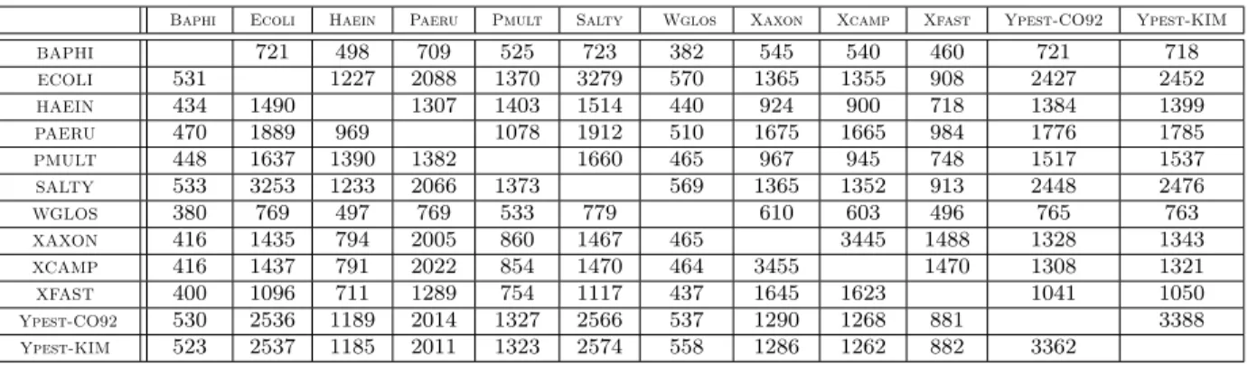
preliminary step, will not be further discussed here. Initially, the sizes of the genomes range from 565 to 5474 genes (see Table 1). Moreover, 8% of the gene families are, on average, duplicated (these duplications cover, on average, 20% of the genes of a genome).
Here, Table 1
5.2
Results
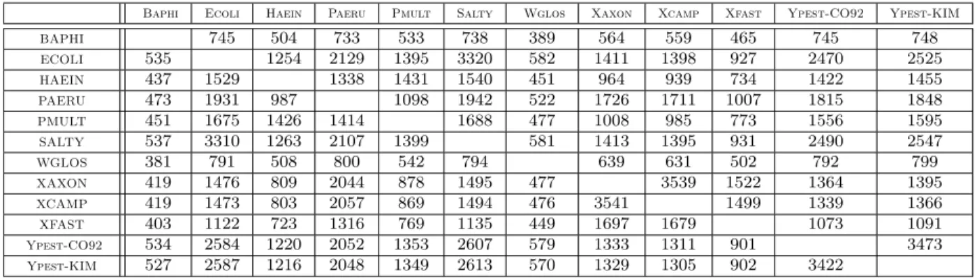
After the pre-processing step (see Section 4.3), 8% of the gene families are, on average, dupli-cated and these duplications cover, on average, 26% of the genes of a genome. Furthermore, pre-processing the dataset by pairs of genomes drastically reduces the size of the genomes. For example, focusing on comparing Baphi and Ecoli, their size reduces from 565 and 4119 genes to 531 and 721, respectively. Table 2 gives all reduced sizes for pairwise compar-isons for the exemplar model and Table 3 gives all reduced sizes for pairwise comparcompar-isons for the maximum matching model. Notice that this latter table also gives all reduced sizes for pairwise comparisons for the intermediate model (indeed, concerning the pre-processing step, a maximum matching can be seen as the “worst” case over all possible intermediate matchings).
Here, Table 3
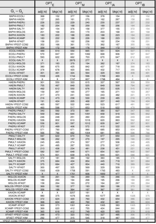
The computation campaign, in which all 0–1 linear programs have been extended with speed-up rules as described in 4.3, has given the results presented in Table 4 (symbol X denotes unsolved instances).
Here, Table 4
Maximum matching model. Recall first that computing the minimum number of break-points and the maximum number of adjacencies for the maximum matching model are equiv-alent problems (see Proposition 1). This problem turned out out to be the easiest case for our γ-Proteobacteria dataset. The CPLEX engine indeed computed all pairwise distances (Table 4) in less than 2 minutes (1.7 second, on average, per pairwise genome comparison).
Exemplar model. Again, recall here that computing the minimum number of breakpoints and the maximum number of adjacencies are equivalent problems for the exemplar model (see Proposition 1). However, oppositely to the maximum matching model, we were not able to compute all pairwise distances. More precisely, 61 out of 66 results (see Table 4) have been obtained thanks to our 0–1 linear programming program in less than 1 minute, except for two cases, for which several hours of computation were necessary. Our attempts for computing the remaining 5 last cases resulted in CPLEX memory exhausted crashes. We note that a similar combinatorial explosion was observed in (Angibaud et al., 2007b) in the
context of maximizing the number of common intervals between two genomes by means of a 0–1 linear program. Unfortunately, we still have no formal explanation for this surprising and counter-intuitive situation. However, we believe this fact to be not related to the CPLEX engine - seen as a black box here.The only obvious observation that can be made for these 5 unsolved cases is that they always take as input two genomes of relatively large sizes (roughly, between 2500 and 3500 genes in each case). However, this is not a sufficient explanation since there are pairs of genomes that have more or less the same size and that went through our program (see for instance Salty/Ypest-KIM). This is why we strongly suspect the structure of the genomes to play a role concerning this problem.
Intermediate model. Recall first that minimizing the number of breakpoints and max-imizing the number of adjacencies are not equivalent problems for the intermediate model. Concerning the problem of maximizing the number of adjacencies, 63 out of 66 results have been obtained in about 3 minutes. As for minimizing the number of breakpoints, 59 out of 66 results have been obtained in less than two minutes.
A justification should be given here for having computed the minimum number of break-points for the intermediate model (problem optIB). Indeed, minimizing the number of break-points for the exemplar and the intermediate models were shown to be equivalent problems in Section 3 (see Proposition 2), and thus the rightmost column of Table 4 might appear just superfluous ; indeed it might be verified in Table 4 that column bkp(M) (exemplar model optE) and column bkp(M) (intermediate model optIB) are always equal. The main reason for having presented both results is to draw the attention of the reader to the fact that, although obtaining the same minimum number of breakpoints as the exemplar model, a matching minimizing the number of breakpoints for the intermediate model might result
in a solution with more adjacencies (see the example at the end of Section 4 for a simple illustration). This could be helpful for obtaining a solution that achieves a double objective: minimizing the number of breakpoints (primary objective) and, among those optimal solu-tions, maximizing the number of adjacencies (secondary objective). This latter goal should be, however, modulated here since the secondary objective is not explicitly stated in the 0–1 linear program, i.e., there is no guarantee that the maximum number of adjacencies is achieved.
We now turn to comparing the results for the different models. First, the following two (average) ratios can be computed from Table 4:
bkpoptE
bkpoptM = 0.89 and
adjoptE
adjoptM = 0.92.
These two ratios illustrate the fact that (i) the minimum number of breakpoints for the exemplar and the maximum matching models differ in about 10%, and (ii) the maximum number of adjacencies for the exemplar and the maximum matching models also differ in about 10%. In the light of these factual ratios, it should thus be emphasized here that, for most practical applications, the choice of the model (exemplar or maximum matching) to focus on should not be underestimated, since noticeable differences might result from this decision.
As for the intermediate model, we already showed that bkpoptE = bkp opt
I . We compare in
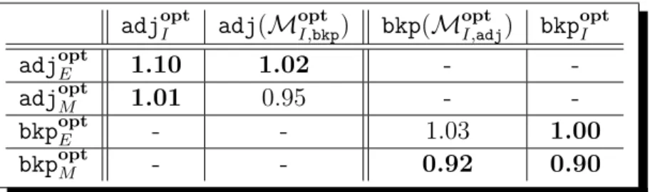
Table 5 the results for the intermediate model with the results for the two other models. To complement Table 5, we indicate in Table 6 how often the same optimal measure (number of breakpoints or number of adjacencies) is found for the intermediate model and for another
model (exemplar or maximum matching). It should be noticed here that, for most cases, we obtain more adjacencies using the intermediate model. The situation is more contrasted when considering the number of breakpoints: for one, we have bkpoptE = bkpoptI (denoted by 100% in Table 6), and for another, for 1/3 of the comparisons, we obtain the same number of breakpoints when maximizing the number of adjacencies for the intermediate model as we obtain for the exemplar model.
Here, Table 5
Here, Table 6
To compare adjoptI and bkp opt
I , the two following (average) ratios can be computed (see
Table 5):
adj(MoptI,bkp)
adjoptI = 0.94 and
bkpoptI
bkp(MoptI,adj) = 0.97.
The intermediate model gives us opportunity to drive the computation with a double objec-tive (minimum number of breakpoints and maximum number of adjacencies). According to the above, one may be tempted to argue that, for the intermediate model, maximizing the number of adjacencies is better than minimizing the number of breakpoints since the obtained solution certainly maximizes the number of adjacencies yet giving about 1/0.97 ≈ 103% of the minimum number of breakpoints (minimizing the number of breakpoints gives about
94% of the maximum number of adjacencies). We however do think that the two ratios are too close to draw any definitive conclusion here on the≪adjopt
I versus bkp
opt
6
Heuristic algorithms
Though our 0–1 linear programming approach presented in Section 4 allows us to obtain almost all the expected exact results in the exemplar, intermediate and maximum matching models on the studied set of γ-Proteobacteria (see Section 5), it should be said that the limits of this method have been attained. Indeed, especially in the intermediate model, some results could not be obtained in reasonable time using this method, and one of the reasons for this is that the sizes of the genomes were too large for the 0–1 linear programming method to be able to handle it. In other words, while this method seems to be promising for “small” genomes (i.e. genomes which, after pre-processing, do not exceed, roughly, two thousand genes), there is a crucial need for faster (and thus not necessarily exact) algorithms in case genomes are of substantially larger sizes ; of course, these heuristic algorithms should provide results of high quality, that is as close as possible from the exact results. In that sense, thanks to the results presented in the previous section, we will be able to compare several heuristics to the exact results and to validate the accuracy of the heuristics provided in this section.
In the following, altogether nine heuristics will be presented and studied (three for each model) ; each of these heuristics fall into one of the two following categories: (i) heuristics based on finding iteratively the Longest Common Subsequence (or LCS, for short) of two genomes, and (ii) heuristics which are a hybrid between category (i) above and the 0–1 linear programming method.
6.1
Description of the Heuristics
Before describing in detail our heuristics, we recall that under the intermediate model, two different problems exist: either we wish to find a matching that maximizes the number of adjacencies, or one that minimizes the number of breakpoints. However, we have seen that minimizing the number of breakpoints in the intermediate model is equivalent to minimizing the number of breakpoints in the exemplar model (see Proposition 2). Thus any heuristic that aims at minimizing the number of breakpoints in the exemplar model will of course apply for minimizing the number of breakpoints in the intermediate model. Consequently, when we turn to the intermediate model, we will only focus on heuristics that aim at maximizing the number of adjacencies.
6.1.1 IILCS heuristics
We first describe here the main ideas that lie behind heuristics based on finding iteratively the Longest Common Subsequence (or LCS, for short), that we have called IILCS heuristics. Let G1 and G2 be two genomes: an LCS of (G1, G2) is a longest common word S of G1 and
G2, up to a complete reversal. The idea here is to match, at each iteration, all the genes
that are present in an LCS, until the desired matching is obtained.
We note that this idea is not new: it has already been used, for instance, in (Marron et al., 2004). In (Angibaud et al., 2007b), this heuristic has been improved in the following way: at each iteration, not only we match all the genes that are contained in an LCS (Rule 1), but we also remove each unmatched gene of a genome for which there is no unmatched gene of same family in the other genome (Rule 2).
Since the difference between the problems lies in the matching that we wish to obtain, our three heuristics will differ on that specific point.
Maximum matching model. We apply iteratively Rule 1 and Rule 2 until the algo-rithm stops. By definition of Rule 1 and Rule 2, this implies that the resulting matching is maximum. We call this heuristic IILCS M.
Intermediate model. We also apply iteratively Rule 1 and Rule 2. The difference here is the stop condition: the algorithm stops as soon as each gene family has been matched at least once. We call this heuristic IILCS IA.
Exemplar model. We apply iteratively Rule 1 and Rule 2 again, but we apply extra deletions of genes at each iteration. Indeed, we need to make sure that only one gene from each family is matched on each genome. In that case, at each iteration, for the duplicate genes which are contained in the current LCS, we arbitrarily keep (and match) the first occurrence ; while for those genes g who are outside LCS, we apply the following rule: if g is present in the LCS (and thus kept in the matching), then we remove all the other occur-rences of g in the rest of both genomes. When this heuristic stops, we are thus guaranteed to obtain an exemplar matching. We call this heuristic IILCS E.
Remark that, for each of those three heuristics, at each iteration, there might exist sev-eral LCS ; in that case, we have decided to randomly choose one of them. Due to this, if one runs IILCS M (respectively IILCS IA, IILCS E) several times on the same instance, it could result in different matchings, and thus the number of breakpoints and adjacencies may vary.
Hence, for each pair of genomes, we have decided to run ten times the heuristics IILCS M, IILCS IA and IILCS E and to keep the best result.
6.1.2 Hybrid method
Let us now describe the other category of heuristics we propose for solving our problems in the three models: this method is a hybrid method using the appropriate IILCS heuristic, followed by the 0–1 linear programming algorithm. The principle is to compute a part of the matching by iterating of the appropriate heuristic IILCS until the size of the LCS is strictly smaller than a given parameter k. Once this is done, we complete the matching by invoking the appropriate 0–1 linear programming algorithm. This heuristic is called HYB M(k) (respectively HYB IA(k), HYB E(k)) in the maximum matching (respectively intermediate, exemplar) model.
For each of the three models, we have tested the hybrid heuristic described above for two different values of k, namely k = 2 and k = 3. We deliberately chose small values of k, because when k gets bigger, invoking the exact algorithm for completing the partial matching might take too long, which is something we want to avoid. Moreover, we will see in the next section that the results obtained with k = 2 and k = 3 are already extremely good.
6.2
Non-exact results
Each of the nine heuristics has been tested on the dataset of γ-Proteobacteria described in Section 5.1. A synthesis of all these results is given in Table 7, where we show, for the nine heuristics, how close they lie to the exact results on average, at worse and at best.
The complete set of results is given in Tables 8, 9 and 10 for problems optM, optIA and optE, respectively. A graphical representation showing, for each problem, how each heuristic
compares to the exact results is provided in Figures 4, 5 and 6 (note that, in each figure, the results are presented in the same arbitrary order than Tables 8, 9 and 10).
Concerning heuristics based on IILCS, their running time is approximately 40 minutes for each of the three problems (we recall that, for each pair of genomes, any given heuristic of this type is run 10 times, thus it takes approximately 4 minutes for each heuristic to achieve all the 66 pairwise comparisons).
As said before, concerning the heuristics based on the hybrid method, we have run them, for each of the three models (i) with parameter k set to 2 and (ii) with parameter k set to 3. The running time, for each of those six heuristics, is roughly five minutes.
Here, Table 7
Here, Figure 4
Here, Figure 5
Here, Table 8
Here, Table 9
Here, Table 10
6.3
Discussion
Globally, the nine heuristics that we have proposed perform very well on our dataset. For each of the three problems, the appropriate IILCS heuristic returns results that are on average at least 90% of the optimal value. It can be seen that IILCS IA is relatively less effective than IILCS E and IILCS M: IILCS IA returns on average results that are 90.56% of the optimal value, while IILCS E (respectively IILCS M) reaches 99.36% (respectively 99%). This can be explained by the fact that IILCS IA, which relies on iteratively finding and matching the genes of a Longest Common Subsequence, is in fact well-fitted for minimizing the number of breakpoints, but not necessarily for maximizing the number of adjacencies. Still, its performances, though not as good as the ones of IILCS E and IILCS M, remain satisfying.
Non surprisingly, our hybrid methods, with parameter k = 2, give better results than their corresponding IILCS heuristics (we are on average 99.48% close to the optimal values for the less effective heuristic). Non surprisingly again, when we set parameter k to 3, the hybrid methods get even better (we are on average 99.82% close to the optimal values for the less effective heuristic). In each case, we are on average closer to the optimal values, and much more exact values are obtained.
There are two main conclusions that can be drawn from this set of results.
First, any of the nine presented heuristics is good on the studied dataset, and in that sense they are all validated. Of course, when possible, better results should be obtained using the hybrid method HYB(3), or HYB(2). However, even after having computed a partial matching by running IILCS down to k = 3 or k = 2, we cannot obtain in reasonable time all results with the 0–1 linear program. In particular, this situation might occur when genomes are of very large sizes. In that case, the good performances of the IILCS heuristics show that they still can be used to obtain fast and accurate results.
Second, these results show that the rather intuitive idea consisting of iteratively finding and matching the genes of a Longest Common Subsequence is very effective for both measures (number of breakpoints and number of adjacencies) and for the three models. It should be said that the same conclusion was drawn in (Angibaud et al., 2007b) concerning the measure “number of common intervals” under the maximum matching model. In that sense, it tends to prove that comparing gene orders should probably, in the future, be studied under this angle.
7
Discussion and future works
This paper developed out of an attempt to build more accurate models for comparative genomics and to design accurate and fast heuristics for breakpoints and adjacencies based measures.
In that sense, the results we have obtained are very satisfying: for one, virtually all the results have been obtained through our 0–1 linear programming approach (though it seems hard to push it further for genomes of larger sizes). For the other, all the heuristics we have proposed perform very well on our dataset.
Another aspect of our work was to focus on the intermediate model. Indeed, our main motivation for this lies on the fact that both the exemplar and the maximum matching might be too restrictive for practical applications. More precisely, if both the exemplar and the maximum matching models provide a clear and simple algorithmic framework, we believe the intermediate model to be well-suited and more accurate for comparative genomics. From this point of view, one of our goals was to observe whether this new model would give very different results from the exemplar and maximum matching models. It turns out that the results are not conclusive: (i) optIBis equivalent to optE(see Proposition 2), and (ii) solving
optIA returns results which, in terms of adjacencies, are relatively close to both optE and optM (see Tables 5 and 6). Hence, studying the pertinence of the intermediate model on
our dataset and for our measures would require a deeper study, and in particular a study of the structure of the output genomes (how many genes of each family are kept and what are their locations, for instance). This specific study is one that we will undertake in the next future.
number of adjacencies, whether the intermediate model radically differs from the others, we still believe this model to be of interest. First, giving more freedom in the structure of the solution is certainly an advantage for practical applications. Second, as illustrated in Table 4, the intermediate model actually gives rise to two combinatorial problems (minimizing the number of breakpoints and maximizing the number of adjacencies). A complementary line of research is thus to develop a 0–1 linear based program for achieving such a double objective. Note that such a program could be obtained by the following procedure: compute the minimum number of breakpoints for the intermediate model, transform this objective into an additional constraint to obtain a modified linear program, and finally compute the maximum number of adjacencies according to the modified 0–1 linear program. Conversely, we can add a constraint to obtain the maximum number of adjacencies, then compute the minimum of breakpoints. These approaches would give us more precise results for the intermediate model than those in Table 4 but its time computation should be more important.
References
Angibaud, S., Fertin, G., and Rusu, I. (2008). On the approximability of comparing genomes with duplicates. In Proc. 2nd Workshop on Algorithms and Computation (WALCOM’08), volume 4921 of LNCS, pages 34–45.
Angibaud, S., Fertin, G., Rusu, I., Th´evenin, A., and Vialette, S. (2007a). A pseudo-boolean programming approach for computing the breakpoint distance between two genomes with duplicate genes. In Proc. 5th RECOMB Comparative Genomics Satellite Workshop (RECOMB-CG’07, volume 4751 of LNBI, pages 16–29.
Angibaud, S., Fertin, G., Rusu, I., and Vialette, S. (2007b). A general framework for com-puting rearrangement distances between genomes with duplicates. Journal of Compu-tational Biology, 14(4):379–393.
Bergeron, A. and Stoye, J. (2003). On the similarity of sets of permutations and its applica-tions to genome comparison. In Proc. 9th International Computing and Combinatorics Conference (COCOON ’03), volume 2697 of LNCS, pages 68–79.
Blin, G., Chauve, C., and Fertin, G. (2004). The breakpoint distance for signed sequences. In Proc. 1st Algorithms and Computational Methods for Biochemical and Evolutionary Networks (CompBioNets), pages 3–16. KCL publications.
Blin, G., Chauve, C., and Fertin, G. (2005). Genes order and phylogenetic reconstruc-tion: Application to γ-proteobacteria. In Proc. 3rd RECOMB Comparative Genomics Satellite Workshop (RECOMB-CG’05), volume 3678 of LNBI, pages 11–20.
Blin, G., Chauve, C., Fertin, G., Rizzi, R., and Vialette, S. (2007). Comparing genomes with duplications: a computational complexity point of view. ACM/IEEE Trans. Com-putational Biology and Bioinformatics, 4(4):523–534.
Blin, G. and Rizzi, R. (2005). Conserved intervals distance computation between non-trivial genomes. In Proc. 11th Annual Int. Conference on Computing and Combina-torics (COCOON’05), volume 3595 of LNCS, pages 22–31.
Bourque, G., Yacef, Y., and El-Mabrouk, N. (2005). Maximizing synteny blocks to identify ancestral homologs. In Proc. 3rd RECOMB Comparative Genomics Satellite Workshop (RECOMB-CG’05, volume 3678 of LNBI, pages 21–35.
Ge-nomics: Empirical and Analytical Approaches to Gene Order Dynamics, Map Align-ment, and the Evolution of Gene Families, pages 207–212. Kluwer.
Chen, X., Zheng, J., Fu, Z., Nan, P., Zhong, Y., Lonardi, S., and Jiang, T. (2005). Assignment of orthologous genes via genome rearrangement. IEEE/ACM Transactions on Computational Biology and Bioinformatics, 2(4):302–315.
Chen, Z., Fowler, R., Fu, B., and Zhu, B. (2006a). Lower bounds on the approximation of the exemplar conserved interval distance problem of genomes. In Proc. 12th Int. Comp. and Combinatorics Conference (COCOON’06), volume 4112 of LNCS, pages 245–254.
Chen, Z., Fu, B., Xu, J., Yang, B.-T., Zhao, Z., and Zhu, B. (2007). Non-breaking simi-larity of genomes with gene repetitions. In Proc. 18th Annual Symposium on Combi-natorial Pattern Matching (CPM’07), volume 4580 of LNCS, pages 119–130.
Chen, Z., Fu, B., and Zhu, B. (2006b). The approximability of the exemplar breakpoint distance problem. In Proc. 2nd International Conference on Algorithmic Aspects in Information and Management (AAIM’06), volume 4041 of LNCS, pages 291–302. Hannenhalli, S. and Pevzner, P. A. (1999). Transforming cabbage into turnip: Polynomial
algorithm for sorting signed permutations by reversals. Journal of the ACM, 46(1):1– 27.
Lerat, E., Daubin, V., and Moran, N. (2003). From gene tree to organismal phylogeny in prokaryotes: the case of γ-proteobacteria. PLoS Biology, 1(1):101–109.
Lerat, E., Daubin, V., Ochman, H., and Moran, N. A. A. (2005). Evolutionary origins of genomic repertoires in bacteria. PLoS Biology, 3(5).
Marron, M., Swenson, K., and Moret, B. (2004). Genomic distances under deletions and insertions. Theoretical Computer Science, 325(3):347–360.
Sankoff, D. (1999). Genome rearrangement with gene families. Bioinformatics, 15(11):909– 917.
Sankoff, D. and Haque, L. (2005). Power boosts for cluster tests. In Proc. 3rd RECOMB Comparative Genomics Satellite Workshop (RECOMB-CG’05), volume 3678 of LNBI, pages 11–20.
Schrijver, A. (1998). Theory of Linear and Integer Programming. John Wiley and Sons. Thach, N. C. (2005). Algorithms for calculating exemplar distances. Honours Year Project
Report, National University of Singapore.
Uno, T. and Yagiura, M. (2000). Fast algorithms to enumerate all common intervals of two permutations. Algorithmica, 26(2):290–309.
Watterson, G. A., Ewens, W. J., Hall, T. E., and Morgan, A. (1982). The chromosome inversion problem. Journal of Theoretical Biology, 99(1):1–7.
Program Adjacency-Maximum-Matching Objective : Maximize P 0≤i<n1 P i<j≤n1 P 0≤k<n2 P k<ℓ≤n2 d(i, j, k, ℓ) Constraints : C.01 ∀ 1 ≤ i ≤ n1, P 1≤k≤n2 |G1[i]|=|G2[k]| a(i, k) = b1(i) ∀ 1 ≤ k ≤ n2, P 1≤i≤n1 |G1[i]|=|G2[k]| a(i, k) = b2(k) C.02 ∀ x ∈ {1, 2}, ∀ g ∈ G, P 1≤i≤nx |Gx[i]|=|g|
bx(i) = min(occ1(g), occ2(g))
C.03 ∀ x ∈ {1, 2}, ∀ 1 ≤ i ≤ j − 1 < nx, cx(i, j) + P i<p<j
bx(p) ≥ 1
C.04 ∀ x ∈ {1, 2}, ∀ 1 ≤ i < p < j ≤ nx, cx(i, j) + bx(p) ≤ 1
C.05 ∀ 1 ≤ i < j ≤ n1, ∀ 1 ≤ k < ℓ ≤ n2,
such that G1[i] = G2[k] and G1[j] = G2[ℓ],
a(i, k) + a(j, ℓ) + c1(i, j) + c2(k, ℓ) − d(i, j, k, ℓ) ≤ 3
C.06 ∀ 1 ≤ i < j ≤ n1,∀ 1 ≤ k < ℓ ≤ n2,
such that G1[i] = G2[k] and G1[j] = G2[ℓ],
a(i, k) − d(i, j, k, ℓ) ≥ 0 a(j, ℓ) − d(i, j, k, ℓ) ≥ 0 c1(i, j) − d(i, j, k, ℓ) ≥ 0
c2(k, ℓ) − d(i, j, k, ℓ) ≥ 0
C.07 ∀ 1 ≤ i < j ≤ n1, ∀ 1 ≤ k < ℓ ≤ n2,
such that G1[i] = −G2[ℓ] and G1[j] = −G2[k],
a(i, ℓ) + a(j, k) + c1(i, j) + c2(k, ℓ) − d(i, j, k, ℓ) ≤ 3
C.08 ∀ 1 ≤ i < j ≤ n1, ∀ 1 ≤ k < ℓ ≤ n2,
such that G1[i] = −G2[ℓ] and G1[j] = −G2[k],
a(i, ℓ) − d(i, j, k, ℓ) ≥ 0 a(j, k) − d(i, j, k, ℓ) ≥ 0 c1(i, j) − d(i, j, k, ℓ) ≥ 0
c2(k, ℓ) − d(i, j, k, ℓ) ≥ 0
C.09 ∀ 1 ≤ i < j ≤ n1, ∀ 1 ≤ k < ℓ ≤ n2,
such that {|G1[i]|, |G1[j]|} 6= {|G2[k]|, |G2[ℓ]|} or G1[i] − G1[j] 6= G2[k] − G2[ℓ],
d(i, j, k, ℓ) = 0 C.10 ∀ 1 ≤ i < j ≤ nP 1, 1≤k<n2 P k<ℓ≤n2 d(i, j, k, ℓ) ≤ 1 Domains : ∀ x ∈ {1, 2}, ∀ 1 ≤ i < j ≤ n1,∀ 1 ≤ k < ℓ ≤ n2,
a(i, k), bx(i), cx(i, k), d(i, j, k, ℓ) ∈ {0, 1}
Figure 1: Program Adjacency-Maximum-Matching for finding the maximum number of ad-jacencies between two genomes under the maximum matching model.
Genome G1 G1[1] G1[2] G1[i − 1] G1[i] G1[i + 1] G1[n1] Genome G2 G2[1] G2[2] G2[k1] G2[kj] G2[kp] G2[n2] |G1[i]| = |G2[k1]| |G1[i]| = |G2[kj]| |G1[i]| = |G2[kp]| a(i, k1) = 0 a(i, kj) = 1 a(i, kp) = 0 b1(i) = 1 b2(k1) ∈ {0, 1} b2(kj) = 1 b2(kp) ∈ {0, 1}
b2(k1) + . . . + b2(kj) + . . . + b2(kp) = min{occ1(|G1[i]|), occ2(|G1[i]|)}
Figure 2: Illustration of the constraints on variable b1(i), 1 ≤ i ≤ n1. If gene G1[i] appears
in positions k1 < k2 < . . . < kp in G2 and gene G1[i] is mapped to gene G2[kj] in the solution
matching, then (i) a(i, kj) = 1, i.e., gene G1[i] is mapped to gene G2[kj], (ii) a(i, kq) = 0
for 1 ≤ q ≤ p and q 6= j, i.e., gene G1[i] is mapped to only one gene in G2, (iii) b1(i) = 1,
i.e., gene G1[i] is mapped to a gene of G2 and (iv) b2(kj) = 1, i.e., gene G2[kj] is mapped
to a gene of G1. Observe that one may have in addition b2(kq) = 1 for some 1 ≤ q ≤ p and
q 6= j if min(occ1(|G1[i]|), occ2(|G1[i]|) ≥ 1 (this observation is however no longer valid for
d(i, j, k, ℓ) = 1 Genome G1 G1[1] G1[i − 1] G1[i] G1[i + 1] G1[j − 1] G1[j] G1[j + 1] G1[n1] Genome G2 G2[1] G2[k − 1] G2[k] G2[k + 1] G2[ℓ − 1] G2[ℓ] G2[ℓ + 1] G2[n2] G1[i] = G2[k] a(i, k) = 1 G1[j] = G2[ℓ] a(j, ℓ) = 1 b1(p) = 0 ∀ i < p < j b1(i) = 1 b1(j) = 1 b2(q) = 0 ∀ k < q < ℓ b2(k) = 1 b2(ℓ) = 1 c1(i, j) = 1 c2(k, ℓ) = 1
Figure 3: Illustration of the constraints on variable d(i, j, k, ℓ), 1 ≤ i < j ≤ n1 and 1 ≤ k <
ℓ ≤ n2, for G1[i] = G2[k] and G1[j] = G2[ℓ]. The two genes G1[i] and G1[j] are adjacent
according to a solution matching if there exist two genes G2[k] and G2[ℓ], G1[i] = G2[k] and
G1[j] = G2[ℓ], such that (i) G1[i] is mapped to G2[k], i.e., a(i, k) = 1, (ii) G1[j] is mapped
to G2[ℓ], i.e., a(j, ℓ) = 1, (iii) no gene between G1[i] and G1[j] is mapped to a gene of G2,
i.e., c1(i, j) = 1 and (iv) no gene between G2[k] and G2[ℓ] is mapped to a gene of G2, i.e.,
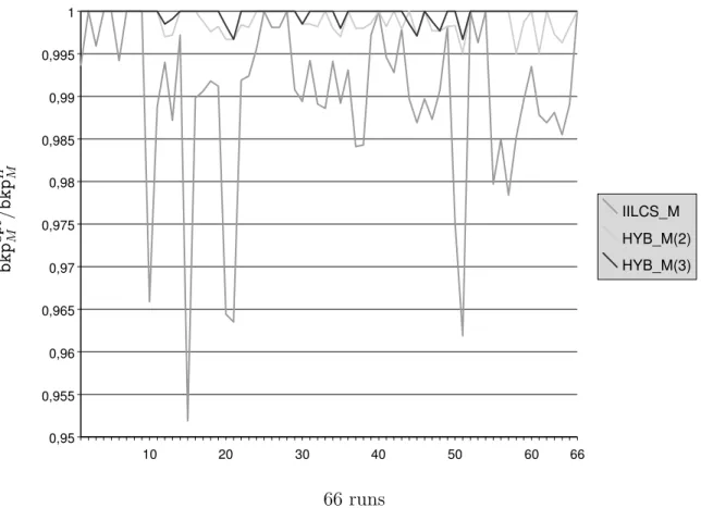
b k p o p t M / b k p H M 10 20 30 40 50 60 66 0,95 0,955 0,96 0,965 0,97 0,975 0,98 0,985 0,99 0,995 1 IILCS_M HYB_M(2) HYB_M(3) 66 runs
Figure 4: Graphical representation of ratio bkpoptM /bkpH
M under the maximum matching
model, for each of the 66 exact results that we have obtained. H is the studied heuristic (i.e., either IILCS M, HYB M(2) or HYB M(3)), bkpH
M is the number of breakpoints computed
by H and bkpoptM is the minimum number of breakpoints under the maximum matching
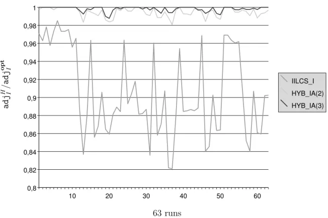
a d j H /I a d j o p t I 10 20 30 40 50 60 0,8 0,82 0,84 0,86 0,88 0,9 0,92 0,94 0,96 0,98 1 IILCS_I HYB_IA(2) HYB_IA(3) 63 runs Figure 5: Graphical representation of ratio adjH
I /adj opt
I under the intermediate model, for
each of the 63 exact results that we have obtained. H is the studied heuristic (i.e., either IILCS IA, HYB IA(2) or HYB IA(3)), adjH
I is the number of adjacencies computed by H and
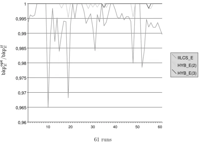
b k p o p t E / b k p H E 10 20 30 40 50 60 0,96 0,965 0,97 0,975 0,98 0,985 0,99 0,995 1 IILCS_E HYB_E(2) HYB_E(3) 61 runs Figure 6: Graphical representation of ratio bkpoptE /bkpH
E under the exemplar model, for each
of the 61 exact results that we have obtained. H is the studied heuristic (i.e., either IILCS E, HYB E(2) or HYB E(3)), bkpH
E is the number of breakpoints computed by H and bkp
opt E is
Genome Baphi Ecoli Haein Paeru Pmult Salty Wglos Xaxon Xcamp Xfast Ypest-CO92 Ypest-KIM
Size 565 4119 1975 5474 1981 4157 642 4105 3939 2631 3540 3788
Baphi Ecoli Haein Paeru Pmult Salty Wglos Xaxon Xcamp Xfast Ypest-CO92 Ypest-KIM BAPHI 721 498 709 525 723 382 545 540 460 721 718 ECOLI 531 1227 2088 1370 3279 570 1365 1355 908 2427 2452 HAEIN 434 1490 1307 1403 1514 440 924 900 718 1384 1399 PAERU 470 1889 969 1078 1912 510 1675 1665 984 1776 1785 PMULT 448 1637 1390 1382 1660 465 967 945 748 1517 1537 SALTY 533 3253 1233 2066 1373 569 1365 1352 913 2448 2476 WGLOS 380 769 497 769 533 779 610 603 496 765 763 XAXON 416 1435 794 2005 860 1467 465 3445 1488 1328 1343 XCAMP 416 1437 791 2022 854 1470 464 3455 1470 1308 1321 XFAST 400 1096 711 1289 754 1117 437 1645 1623 1041 1050 Ypest-CO92 530 2536 1189 2014 1327 2566 537 1290 1268 881 3388 Ypest-KIM 523 2537 1185 2011 1323 2574 558 1286 1262 882 3362
Table 2: Reduced sizes of the genomes for pairwise comparisons under the exemplar model. As an illustration, pre-processing the data for comparing Baphi with Ecoli reduces in two genomes of size 531 (Baphi) and 721 (Ecoli).
Baphi Ecoli Haein Paeru Pmult Salty Wglos Xaxon Xcamp Xfast Ypest-CO92 Ypest-KIM BAPHI 745 504 733 533 738 389 564 559 465 745 748 ECOLI 535 1254 2129 1395 3320 582 1411 1398 927 2470 2525 HAEIN 437 1529 1338 1431 1540 451 964 939 734 1422 1455 PAERU 473 1931 987 1098 1942 522 1726 1711 1007 1815 1848 PMULT 451 1675 1426 1414 1688 477 1008 985 773 1556 1595 SALTY 537 3310 1263 2107 1399 581 1413 1395 931 2490 2547 WGLOS 381 791 508 800 542 794 639 631 502 792 799 XAXON 419 1476 809 2044 878 1495 477 3539 1522 1364 1395 XCAMP 419 1473 803 2057 869 1494 476 3541 1499 1339 1366 XFAST 403 1122 723 1316 769 1135 449 1697 1679 1073 1091 Ypest-CO92 534 2584 1220 2052 1353 2607 579 1333 1311 901 3473 Ypest-KIM 527 2587 1216 2048 1349 2613 570 1329 1305 902 3422
Table 3: Reduced sizes of the genomes for pairwise comparisons under the maximum match-ing and intermediate models. As an illustration, pre-processmatch-ing the data for comparmatch-ing Baphi with Ecoli reduces in two genomes of size 535 (Baphi) and 745 (Ecoli).
BAPHI-ECOLI 368 152 377 156 378 154 372 152 BAPHI-HAEIN 157 265 161 270 162 267 158 265 BAPHI-PAERU 226 232 229 240 230 237 227 232 BAPHI-PMULT 182 254 188 259 189 256 184 254 BAPHI-SALTY 367 154 376 158 377 155 372 154 BAPHI-WGLOS 201 168 203 170 203 168 201 168 BAPHI-XAXON 183 222 188 226 188 223 184 222 BAPHI-XCAMP 183 222 188 226 188 223 183 222 BAPHI-XFAST 158 231 162 236 162 234 158 231 BAPHI-YPEST-CO92 352 166 361 170 362 167 355 166 BAPHI-YPEST-KIM 339 172 348 176 349 172 343 172 ECOLI-HAEIN 489 610 550 665 551 624 507 610 ECOLI-PAERU 570 847 651 1082 668 906 597 847 ECOLI-PMULT 593 622 662 703 670 647 612 622 ECOLI-SALTY X X 2875 277 X X X X ECOLI-WGLOS 371 183 379 194 382 187 374 183 ECOLI-XAXON 380 675 425 842 437 718 390 675 ECOLI-XCAMP 378 678 420 845 432 717 386 678 ECOLI-XFAST 301 491 324 564 329 503 308 491 ECOLI-YPEST-CO92 1559 426 1744 596 1789 463 X 426 ECOLI-YPEST-KIM X X 1747 607 1798 464 X X HAEIN-PAERU 301 550 333 615 337 567 309 550 HAEIN-PMULT 755 497 849 525 849 509 794 497 HAEIN-SALTY 492 612 550 676 553 635 515 612 HAEIN-WGLOS 159 267 165 277 165 271 163 267 HAEIN-XAXON 217 473 241 533 243 482 221 473 HAEIN-XCAMP 216 473 238 530 239 485 218 473 HAEIN-XFAST 191 424 205 468 207 440 194 424 HAEIN-YPEST-CO92 465 597 522 649 523 617 481 597 HAEIN-YPEST-KIM 460 598 517 653 518 622 479 598 PAERU-PMULT 340 592 373 681 380 627 347 592 PAERU-SALTY 559 862 644 1091 658 918 585 862 PAERU-WGLOS 246 248 251 260 253 249 249 248 PAERU-XAXON 536 802 610 1016 620 863 562 802 PAERU-XCAMP 536 801 597 1012 609 847 557 801 PAERU-XFAST 372 499 406 572 410 522 389 499 PAERU-YPEST-CO92 571 790 671 990 685 853 604 790 PAERU-YPEST-KIM 566 786 662 1004 681 855 598 786 PMULT-SALTY 597 622 670 704 677 650 620 622 PMULT-WGLOS 188 262 197 270 197 265 190 262 PMULT-XAXON 245 495 274 557 277 506 248 495 PMULT-XCAMP 241 495 267 555 270 507 245 495 PMULT-XFAST 213 436 234 481 238 451 221 436 PMULT-YPEST-CO92 582 597 648 671 654 621 602 597 PMULT-YPEST-KIM 574 601 639 676 644 631 588 601 SALTY-WGLOS 372 181 380 192 383 185 376 181 SALTY-XAXON 375 684 434 854 445 718 391 684 SALTY-XCAMP 375 684 427 854 440 716 389 684 SALTY-XFAST 300 497 325 569 329 509 310 497 SALTY-YPEST-CO92 1560 439 1758 591 1793 483 X 439 SALTY-YPEST-KIM X X 1761 606 1800 477 X X WGLOS-XAXON 189 261 194 269 195 266 189 261 WGLOS-XCAMP 189 260 194 268 195 266 189 260 WGLOS-XFAST 158 264 163 272 164 267 160 264 WGLOS-YPEST-CO92 369 182 377 193 380 186 373 182 WGLOS-YPEST-KIM 356 186 364 197 367 187 361 186 XAXON-XCAMP X X 3257 181 X X X X XAXON-XFAST 980 375 1076 400 1077 380 1026 375 XAXON-YPEST-CO92 372 624 420 760 432 654 386 624 XAXON-YPEST-KIM 368 624 422 760 432 661 385 624 XCAMP-XFAST 969 373 1061 404 1065 383 1005 373 XCAMP-YPEST-CO92 369 620 412 755 424 644 380 620 XCAMP-YPEST-KIM 365 618 412 749 420 655 379 618 XFAST-YPEST-CO92 298 473 323 542 327 485 306 473 XFAST-YPEST-KIM 292 477 315 545 318 487 298 477 YPEST-CO92-YPEST-KIM X X 3328 59 X X X X OPT
E OPTM OPTIA OPTIB
G1 – G2 adj(M) bkp(M) adj(M) bkp(M) adj(M) bkp(M) adj(M) bkp(M)
Table 4: Number of adjacencies adj(M) and number of breakpoints bkp(M) for problems optE, optM, optIA and optIB. M always denotes the returned solution and X stands for the unsolved cases.
adjoptI adj(MoptI,bkp) bkp(MoptI,adj) bkpoptI
adjoptE 1.10 1.02 -
-adjoptM 1.01 0.95 -
-bkpoptE - - 1.03 1.00
bkpoptM - - 0.92 0.90
Table 5: Comparison of the results for adjoptI : maximum number of adjacencies for the inter-mediate model, adj(MoptI,bkp): number of adjacencies induced by a matching MoptI,bkp yielding the minimum number of breakpoints for the intermediate model, bkp(MoptI,adj): number of
breakpoints induced by a matching MoptI,adj yielding the maximum number of adjacencies for the intermediate model, bkpoptI : minimum number of breakpoints the intermediate model, adjoptE : maximum number of adjacencies for the exemplar model, adjoptM : maximum num-ber of adjacencies for the maximum matching model, bkpoptE : minimum number of break-points for the exemplar model, bkpoptM : minimum number of breakpoints for the maximum matching model. Bold values indicate cases where the intermediate model performs better than the exemplar or maximum matching model. Shown here are the average ratios, e.g.,
adjoptI
adjoptE
= 1.10, and hence, on average, the number of adjacencies for the exemplar model is about 1/1.10 = 90% of the number of adjacencies achieved by the intermediate model.
adjoptI adj(MoptI,bkp) bkp(MoptI,adj) bkpoptI
adjoptE 0% 9% -
-adjoptM 11% 0% -
-bkpoptE - - 3% 100%
bkpoptM - - 0% 0%
Table 6: Shown here is the percentage that the same optimal measure (maximum number of adjacencies and minimum number of breakpoints) is found for the intermediate models and the two other models (exemplar and maximum matching). For example, for 5 out of 58 pairs of genomes i.e., 9%, it holds that adjoptE = adj(MoptI,bkp) (see Table 5).
![Figure 2: Illustration of the constraints on variable b 1 (i), 1 ≤ i ≤ n 1 . If gene G 1 [i] appears in positions k 1 < k 2 <](https://thumb-eu.123doks.com/thumbv2/123doknet/11574025.297717/42.918.104.791.101.419/figure-illustration-constraints-variable-gene-g-appears-positions.webp)