Determination of Young's modulus of mandibular bone using inverse analysis

HAL Id: hal-00509752

https://hal-mines-paristech.archives-ouvertes.fr/hal-00509752

Submitted on 9 Mar 2012

HAL is a multi-disciplinary open access

archive for the deposit and dissemination of

sci-entific research documents, whether they are

pub-lished or not. The documents may come from

teaching and research institutions in France or

abroad, or from public or private research centers.

L’archive ouverte pluridisciplinaire HAL, est

destinée au dépôt et à la diffusion de documents

scientifiques de niveau recherche, publiés ou non,

émanant des établissements d’enseignement et de

recherche français ou étrangers, des laboratoires

publics ou privés.

using inverse analysis

Guillaume Odin, Charles Savoldelli, Pierre-Olivier Bouchard, Yannick Tillier

To cite this version:

Guillaume Odin, Charles Savoldelli, Pierre-Olivier Bouchard, Yannick Tillier.

Determination of

Young’s modulus of mandibular bone using inverse analysis. Medical Engineering and Physics,

Else-vier, 2010, 32 (6), pp.Pages 630-637. �10.1016/j.medengphy.2010.03.009�. �hal-00509752�

DETERMINATION OF YOUNG'S MODULUS OF MANDIBULAR BONE USING INVERSE ANALYSIS

Guillaume Odin, M.D., Ph.D.; Charles Savoldelli, M.D.; Pierre-Olivier Bouchard, Ph.D.; Yannick Tillier, Ph.D.

Abstract

Development of a numerical model applicable to clinical practice, and in particular oral implantology, requires knowledge of the mechanical properties of mandibular bone. The wide range of mechanical parameters found in the literature prompted us to develop an inverse analysis method that takes into account the exact geometry of each specimen tested, regardless of its shape. The Young's modulus of 3000 MPa we determined for mandibular bone using this approach is lower than the values reported in the literature. This difference can be explained by numerous experimental factors, related in particular to the bone specimens used. However, the main reason is that, unlike most previously published papers on the subject, the heterogeneity of bone led us to select a specimen size at the upper end of the scale, close to clinical reality.

1 Introduction

Dental implants are an effective and commonly used treatment for the replacement of lost teeth and rehabilitation after maxillo-facial trauma. The current objective of clinical research is to simplify this kind of surgery while achieving a long-lasting result. The finite element method (FEM) plays an important role today in solving engineering problems in many fields of science and industry. It can also be successfully applied for the simulation of biomechanical systems and dental implants (Chuong et al., 2005; Savoldelli et al., 2008).

However, the development of such FEM models requires specific knowledge of the mechanical properties of both the mandible and implants. Numerous studies have been conducted on the mechanical behaviour of titanium implants, but determination of the biomechanical properties of living tissues or bone remains challenging. The wide range of values published in the literature for Young’s modulus of human bones confirms this situation. We propose a new approach for identification of rheological parameters using an inverse analysis method based on comparison of computed results of compression tests and actual experimental findings.

The Young’s modulus obtained for bone specimens can differ considerably, depending on the mechanical test used. This can be explained not only by the mechanical properties of bone, such as anisotropy, but also by the mechanical test itself. Many parameters influence the determination of mechanical or physical properties: specimen size, the way the specimen has been stored and tested, specimen shape, loading conditions (static or dynamic), and, obviously, the experimental means. As reported by Bosisio et al. (2007), the Young’s modulus determined by biomechanical testing at the midshaft of long bones, mainly the femur, for a large number of specimens (regularly shaped reduced section or cubic specimens) varies between 8 and 22.8 GPa.

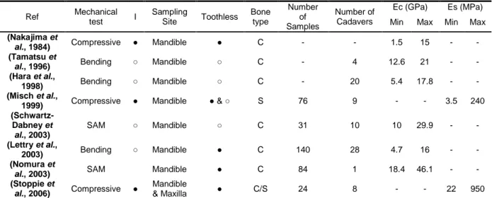
More specifically, Table 1 summarizes the results of several major studies on jawbones. These studies were carried out on standardized specimens from cadaver jawbones using three different kinds of mechanical tests: compressive test, 3-point bending method, and techniques relying on Scanning Acoustic Microscopy (SAM). Some of the studies took bone anisotropy into account (Hara

et al., 1998; Lettry et al., 2003; Schwartz-Dabney et al., 2003; Tamatsu et al., 1996). The values obtained for Young’s modulus are widely dispersed and vary between 1.5 and 29.8 GPa.

Table 1 - Discrepancy among values of Young’s modulus (Ec & Es) for cortical (C) and cancellous (S) jawbone found in the literature; I, isotropic; ●, Yes; ○, No

Ref Mechanical test I Sampling Site Toothless Bone type Number of Samples Number of Cadavers Ec (GPa) Es (MPa) Min Max Min Max

(Nakajima et

al., 1984) Compressive ● Mandible ● C - - 1.5 15 - -

(Tamatsu et

al., 1996) Bending ○ Mandible ○ C - 4 12.6 21 - -

(Hara et al.,

1998) Bending ○ Mandible ○ C - 20 5.4 17.8 - -

(Misch et al.,

1999) Compressive ● Mandible ● & ○ S 76 9 - - 3.5 240

(Schwartz-Dabney et al., 2003) SAM ○ Mandible ○ C 31 10 10 29.9 - - (Lettry et al., 2003) Bending ○ Mandible ● C 140 28 4.7 16 - - (Nomura et

al., 2003) SAM Mandible ● C 84 1 18.4 46.1 - -

(Stoppie et

al., 2006) Compressive ●

Mandible

& Maxilla ● C/S 24 8 - - 22 950

It is therefore of prime importance to fully define the mechanical test (specimen shape, size, etc.) used in a study and to specify how accurate the results are in order to permit reliable interpretation.

Determination of Young’s modulus is generally based on the stress/strain curves obtained analytically from the experimental load/displacement curves. The problem is that this analytical transformation is often based on very strong hypotheses such as material homogeneity, isotropic behaviour, isothermal conditions, etc. as well as on standardized specimen shapes. For biomaterials, this requires a fastidious machining step (mainly cutting) that can adversely affect specimen quality. For instance, specimens can be damaged during machining, and the scale on which the specimens are going to be tested may be not as representative as it should be of the jawbone as a whole.

This study was conducted using inverse analysis techniques that allow characterization of material parameters using non-standardized specimens. Inverse analysis approaches are based on comparison of the curves resulting from a mechanical test with those obtained by numerical simulation of the same test using reliable simulation software. The main advantage of this approach is that it eliminates the need to machine the specimens; the biomaterial constitutive equations are determined directly from bone specimens of variable sizes and shapes. In particular, material characterization can

be performed using the same scale as that on which the system will be modelled later on. This eliminates any problems due to extrapolation.

2 Materials and methods

The choice of adequate constitutive (and friction) laws is essential to obtain satisfactory numerical results. As shown in Fig. 1, the inverse model we propose is designed to estimate mechanical parameters from inhomogeneous mechanical tests. This method is based on comparison of the data obtained from measurements with the results obtained using a direct numerical model (FORGE 2005®) that was initially dedicated to the simulation of forming processes and then adapted to surgical simulation.

Sample preparation CT scan of the sample

Mechanical test (compressive test)

3D finite element mesh generation of the sample

Direct model Numerical simulation Parameters optimisation Experimental curves Load (N) vs Displacement (mm)

E (MPa)

2.1 Experimental work

2.1.1 Specimen preparation

Mandibular bone samples were collected without soft tissues from fresh cadavers and were stored at -20 °C. Specimens of both cancellous and cortical bone measuring approximately -20 mm in width and 30 to 40 mm in height were obtained by sectioning with a Lindemann bur. Irrigation with a saline solution (9 %o) was performed to minimize any damage due to heating. A total of 4 to 6 specimens were collected from each mandible (Fig. 2).

Fig. 2 - Mandible specimen preparation

Each piece was hollowed out with a dental bur in a saline solution (9 %o) to eliminate the cancellous bone; this provided specimens of mandibular cortical bone. Because our ultimate goal was to create a numerical model capable of predicting the behaviour of the system formed by the bone and an implant, we decided to study the dentate portion of the mandible, and in particular the symphysis and the horizontal branches. The bone specimens were stored in a cooler during their transfer, before CT-scan analysis and mechanical tests. As shown in Table 2, 41 specimens were collected from nine mandibles from 5 women and 4 men (average donor age 79.55 years). The specimens were tested on an Instron® testing machine (see §2.1.3).

Table 2 - Number of samples / mandibles collected (W: Women / M: Men)

Number n sex Age (mean value) n samples

Mandibles 9 5W, 4M 79.55 yr 41

Hydration of the specimens was not checked during the mechanical tests.

In order to validate our approach, two radius specimens obtained from two separate cadavers (75 and 96 years) were also tested in order to compare the Young’s modulus identified using our procedure with those published by Bosisio et al. (2007) for cortical radius bones (Table 2).

2.1.2 3D bone mesh generation

2D DICOM images of the bone specimens were obtained using a medical CT unit (Fig. 3a). For each specimen, 600 mm thick slices were recorded every 300 m along a perpendicular axis.

3D segmentation AMIRA 3D® software was used to generate surface mesh models of the jawbones directly from clinical imaging data (Fig. 3b). The .unv files generated were then imported into our own finite element software in order to generate full 3D volumic tetrahedral meshes for each bone specimen (Fig. 3c).

(a) (b) (c)

Fig. 3 - 3D model preparation ; (a) Medical CT-scan image, (b) Surface mesh model, (c) 3D volume mesh

2.1.3 Mechanical test

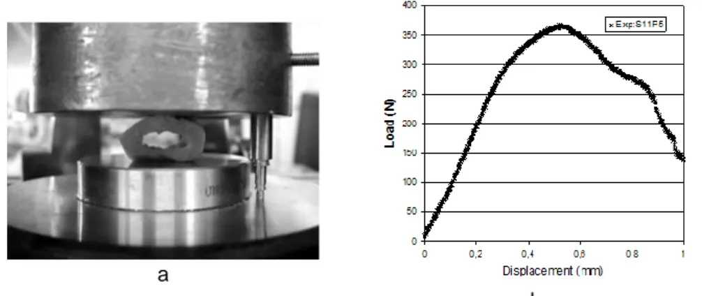
The experimental device used for material behaviour characterization is a standard pneumatic tensile-testing machine (Instron® 1121) capable of performing compressive tests with a force sensor of 10 kN. An LVDT extensometer was used to improve measurement accuracy (Fig. 4a). A preload of approximately 10 N was applied to the specimens.

Specimen alignment on the test platens is based on a three-point contact pattern. Local plasticization and overall deformation can cause specimen rotation. In order to enable accurate replication of the experimental conditions in the numerical model, photographs and movies were taken before, during,

and after the test. Post-controls did not reveal any macroscopic modifications of the specimens in the areas in contact with the test platens.

Fig. 4b shows a typical compression curve obtained using this experimental setup. At first, the force increases linearly. The slope of the curve then starts to decrease due to material damage. At this point, cracks start to appear. Once the maximum is reached, the specimen’s structure breaks and the curve decreases.

a

b

Fig. 4 - Mechanical test; (a) Compression test using an LVDT extensometer, (b) Load vs. Displacement curve

2.2 Numerical simulation

The numerical software used to model the compression tests was FORGE 2005®, a program that was developed in our laboratory.

2.2.1 The direct model

The direct model FORGE 2005® software used for mechanical simulation of the experimental test consists of a 3D finite element model that was originally developed for material forming. It is based on an updated Lagrangian formulation suitable for large deformations, and takes into account evolving contact conditions with tools.

As a first approximation, the mechanical behaviour of bones can be considered linear-elastic if the relative displacement with respect to the specimen size is small.

ε

I

ε

σ

trace

2

where and are the Lamé coefficients, I the unit tensor, and the Cauchy stress tensor. is the strain tensor defined from the displacement field u:

u

grad

u

grad

Equation (1) can be rewritten:

tr

p

e

s

.

2

where s and e are respectively the deviatoric stress and strain tensors and is the compressibility coefficient. Linear-elastic incompressibility is expressed by:

0

u

div

trace

When gravity forces are included and the forces of inertia are neglected as a first approximation, the equilibrium equation is written:

0

g

p

grad

s

div

g

div

and the problem must be solved in terms of the unknown fields u and p.

There are three main kinds of boundary conditions for this problem:

- a kinematic boundary condition, due to the prescribed displacement of the compressive machine die,

- a stress-free boundary condition on the free surface of the specimens, - a non-penetration contact condition between the die and the specimens.

0

*

0

*

*

*

:

dV

p

u

div

p

dV

gv

dV

v

pdiv

dV

s 

A weak formulation of the mechanical problem can be obtained using the virtual work principle. A mixed finite element P1+/P1 in velocity/pressure is used to discretize the problem (Coupez et al., 1991; Arnold et al., 1984). This mixed formulation makes these linear tetrahedral elements insensitive to spurious stress-locking effects.

Since it is highly non-linear, mainly due to unilateral contact conditions, it is solved using a Newton-Raphson algorithm. Once mechanical equilibrium is reached, a Lagrangian update procedure is used with an explicit Euler integration scheme.

An automatic remeshing algorithm is used to prevent mesh degeneration for high strains (Coupez et al., 1991). This finite element code can accurately simulate mechanical tests. It reveals the evolution of certain measurable data such as force vs. time or displacement. The crosshead velocity is assumed to be constant and known.

2.2.2 The inverse model: parameter identification

The inverse method aims at fitting computed data to experimental data by finding the optimal set of constitutive parameters (Young’s modulus in our case). This problem is formulated as a least squares problem (Favennec et al., 2002, Tillier et al., 2006):

NbM i E xp i NbM i E xp i Com p i opt opt

M

M

E

M

E

E

Min

E

E

with

as

such

Find

where is the objective function,

M

M

experimental measurement, NbM the number of measurements, and a constraint space. A statistical interpretation of this problem is obtained by considering that the experimental measurement can be expressed as the results of the direct model plus an error (measurement error) ei:

true Comp i Exp i i

M

M

E

e

This implies the existence of an “exact” value of E (denoted Etrue). The error due to the choice of the model is assumed to be negligible.

2.3 Boundary conditions

A dedicated preprocessor allows definition of all of the boundary conditions required for simulation. They must be the same as the experimental boundary conditions in order to make the approach accurate.

The geometry of each specimen was imported from CT-scan data, as shown in § 2.1.2. As a first approximation, the mechanical behavior of jawbone was defined as homogenous and isotropic and was modeled using a linear-elastic constitutive equation. Poisson’s coefficient ( ) was constant and equal to 0.3, meaning that the bone is assumed to be partly compressible. The initial value of Young’s modulus was arbitrarily set at 5 000 MPa. An adiabatic heat exchange condition was applied and the room temperature was set at 20 °C.

The compression machine platens were modeled using two non-deformable parallelepipeds: the lower die and the press itself. The contact between the specimens and the dies was modeled using a Tresca friction law with a high friction parameter (friction parameter set at 0.4). This parameter must be set as close as possible to reality as it may alter the modeling result. For example, a sliding contact tends to reduce the slope of the load vs. displacement curve whereas a sticking contact will increase it. Total displacement was set at 0.8 mm. For higher values, some damage is noticeable experimentally. Since no damage criteria are taken into account in the numerical model, it is better to limit the displacement to the undamaged area to avoid non-exploitable data and thus reduce the computing time.

Each numerical specimen was positioned on the lower die using a center of gravity as close as possible to that of the experimental position by comparison with the photographs and movies taken during the compression test. The same preloading condition as that used experimentally was applied to the specimens to avoid any undesirable movement (Fig. 5a and 5b).

(a) (b)

3 Results

Simulation of each specimen compression test was performed using a manual optimization approach in which Young’s modulus was modified until the numerical load vs. displacement curves perfectly fit the experimental curves.

The last Young’s modulus, which minimized the gap between the curves (less than 0.5 %), was considered representative of the specimen studied (Fig. 6).

Fig. 6 - Inverse analysis results. Best result obtained using N=3000 MPa.

Comparison of the curves was restricted to their linear portion. For each value of Young’s modulus E, the objective function was computed using the least squares problem (7). Optimization was performed using only one observable: the load. Compression tests were performed in two different directions, as shown in Fig. 7a and 7b. Table 3 shows the results obtained for the entire set of specimens.

Fig. 7 - Compression tests performed in two different directions (a) and (b) Table 3 -Young’s modulus values E (MPa) determined for each sample

Samples Mandible EM1 EM 2 E M3 EM4 EM5 EM6 EM7 EM8 EM9 S1 2000 (x) - 3500 (x) 2000 (x) 4000 (x) 4500 (x) 2000 (x) 4000 (y) 3000 (y) S2 - 5000 (x) 3000 (x) 2000 (x) 4000 (x) 3000 (x) 2000 (x) 3500 (y) 2000 (y) S3 2000 (x) - 3000 (y) - 4500 (x) 3000 (x) 2500 (x) 3000 (x) 3000 (y) S4 - 4000 (y) 3000 (x) 2000 (x) 4000 (x) 3000 (x) 2000 (x) 2500 (x) 3000 (x) S5 2000 (x) 4000 (x) - 3000 (x) 3000 (x) 2500 (x) 2500 (x) 3000 (x) 2000 (x) S6 2000 (x) Max 2000 5000 3500 3000 4500 4500 2500 4000 3000 Min 2000 4000 3000 2000 3000 2500 2000 2500 2000 Emean ( SD) 2000 (0) 4333,3 (577,3) 3125 (250) 2250 (500) 3900 (547,7) 3200 (758,2) 2200 (273,8) 3200 (570,08) 2600 (547,7) Radius ER1 ES2 S1 15 000 10 000

EMZ: Z stands for the mandible number.

ERZ: Z stands for the radius number.

S#: # stands for the sample number for mandible or radius number Z.

(x) and (y) show the test direction axis.

The mean value of E obtained after 40 evaluations was 2894 +/- 685 MPa in the x direction and 3214 +/- 699 MPa in the y direction. The overall mean value (taking into account both directions) was 2980 +/- 794 MPa. Young’s modulus for the two radius specimens was respectively 15 and 10 GPa.

As shown in Fig. 8, two different mandible compression tests were simulated using the identified parameters. Numerical results agreed well with the experimental results in terms of both stress and deformation levels. The stress peaks were predicted exactly in the areas where cracks appeared experimentally at comparable force levels.

Case 1

Case 2

Fig. 8 - Validation test: comparison between simulation and experiments for two compression directions

4 Discussion

For the two radius specimens, Young’s modulus in one case (15 GPa) was of the same order of magnitude as those found by Bosisio et al. (2007), whereas the second result was lower (10 GPa). The mean value of Young’s modulus for the mandible obtained for the entire set of tests was approximately 3 GPa, which is much lower than most of the values found in the literature, especially those used for finite element modeling of the jawbone (~ 15 GPa). This paragraph explains why our value was lower than expected but nevertheless gives good results.

4.1 Sampling location

Schwartz-Dabney et al. (2003) demonstrated significant regional variability in the material properties of the human dentate mandible. In their study, specimens were taken from the ramus of the mandible, a region that is more cortical than the dentate area. This might explain the considerable difference in the Young’s modulus determined.

4.2 Mechanical testing

The unconfined mechanical compression test we used, which was adapted to the size of our bone specimens, may be responsible for a loss of continuity and can lead to underestimation of Young’s modulus (Linde et al., 1989). It has previously been established that the compression tests designed to measure the elastic modulus of trabecular bone suffer from several experimental artifacts, and in particular so-called “end-artifact” (Keaveny et al., 1997) and “side-artifact” errors (Ün et al., 2006 and). With simple cylindrical specimens, such artifacts have been shown to affect the estimated Young’s modulus by up to 20-30% (Allard et al., 1991) compared to total specimen deflection with extensometer measurements from the middle sections of 10 mm3 specimens. The stiffness determined for the middle part was considerably greater than that from total deflection. Nevertheless, this effect decreased as specimen size increased, and even disappeared for larger sizes. This effect was relatively limited in this study owing to the size of our specimens (20 mm width x 30-40 mm height).

4.3 Cadaver age and influence of tooth loss on material properties

For Schwartz-Dabney et al. (2002), edentulation alters the material properties of cortical bone in the human mandible. According to these authors, compared with the dentate mandible, the edentulous mandible has on average:

greater maximum stiffness coupled with thicker bone in the lingual corpus,

greater maximum stiffness anteriorly in the facial corpus and at the lingual condylar neck, lesser maximum stiffness and thickness in portions of the ramus,

different directions of the axes of maximum stiffness at some sites, especially in the buccal retromolar region.

4.4 Degree of bone hydration

Dehydration of bone specimens increases their Young’s modulus by 15% to 30% (Linde et al., 1993). In our study, the test specimens were taken from fresh cadavers, which minimized this factor.

4.5 Test temperature

As for most biological materials, the mechanical properties of bone depend on the temperature. While it would have been preferable to perform the tests at 37°C (body temperature), this would have involved numerous methodological problems. However, the influence of the temperature is negligible for static tests (Bonfield et al., 1968; Carter et al., 1976), which was the case in our study.

4.6 Specimen storage

Freezing affects the mechanical properties of bone at a temperature of -70°C (Nomura et al., 2003). However, no effect has been demonstrated at a temperature of -20°C. Furthermore, it has been shown that post-mortem sampling does not modify the properties of bone if performed before 120 days (Stevens et al., 1962).

4.7 Bone anisotropy

The anisotropy of mandibular bone manifests as a progressive reduction of Young’s modulus the greater the distance from the longitudinal strain axis (Tamatsu et al., 1996, Ichim et al., 2006, Lettry et al., 2003). These results are compatible with those obtained for the long bones. The strain axis used in our study formed a 90° angle with the longitudinal axis, corresponding to the principal axis of masticatory strain.

4.8 Bone porosity

An increasing linear relationship exists between bone density and Young’s modulus (Carter et al., 1978; Cowin et al., 2001). However, the precision of the CT units used for acquisition of the images required for the numerical phase of analysis is not accurate enough to isolate the smallest zones of spongy cancellous bone, namely at the interface with the cortical bone. Certain zones are thus fitted with a finite element mesh like that of cortical bone, whereas the true anatomic specimen actually probably contains small zones of spongy cancellous bone. The result is underestimation of the calculated Young’s modulus. Data acquisition can be improved using microtomography. However, this technique, available for research purposes, cannot be used in clinical practice, and thus cannot be applied to implantology at the present time.

5 Conclusion

Knowledge of the mechanical properties of mandibular bone is necessary for development of a numerical model applicable to clinical practice, and in particular oral implantology. The wide range of mechanical parameters published in the literature led us to develop an inverse analysis method that takes into account the exact geometry of each specimen tested, regardless of its shape. The Young’s modulus of 3000 MPa determined for mandibular bone in our study using this approach is lower than the values reported in the literature. This difference can be explained by numerous experimental factors related in particular to the bone specimens used (type of bone, donor age, and storage conditions). The main reason, however, is that, unlike most existing papers on the subject, the specimen dimensions were defined at the upper end of the scale, close to clinical reality. On this scale, bone is a composite material composed primarily of cortical bone but with some cancellous bone inclusions. The macroscopic constitutive representation proposed in this paper is a sufficiently accurate model to represent a mean constitutive response.

6 References

Allard, F., and Ashman, R., 1991. A comparison between cancellous bone compressive moduli determined from surfaced strain and total specimen deflection. Orth Res Soc 16:151.

Arnold, D.N., Brezzi, F., Fortin, M., 1984. A stable finite element for the Stokes equations. Calcolo 21, 337-344.

Bonfield, W., and Li, C. H., 1968. The temperature dependence of the deformation of bone. J Biomech 1, 323-9.

Bosisio, M. R., Talmant, M., Skalli, W., Laugier, P., and Mitton, D., 2007. Apparent Young's modulus of human radius using inverse finite-element method. J Biomech 40, 2022-8.

Carter, D. R., Hayes, W. C., 1976. Fatigue life of compact bone-I. Effects of stress amplitude, temperature and density. J Biomech 9:27-34.

Carter, D. R., Spengler, D. M., 1978. Mechanical properties and composition of cortical bone. Clin Orthop Relat Res, 192-217.

Chuong C., Borotikar B., Schwartz-Dabney C., Sinn D., 2005. Mechanical characteristics of the mandible after bilateral sagittal split ramus osteotomy: Comparing 2 different fixation techniques. J Oral Maxillofac Surg 63(1), 68-76

Coupez, T., 1991. Grandes deformations incompressibles - remaillage automatique, PhD. thesis, ENSMP, Sophia Antipolis, France.

Favennec, Y., Labbé, V., Tillier, Y., Bay, F., 2002. Identification of magnetic parameters through inverse analysis coupled with finite element modeling. IEEE Transaction on Magnetics 38 (6), 3607-19.

Hara, T., Takizawa, M., Sato, T., and Ide, Y., 1998. Mechanical properties of buccal compact bone of the mandibular ramus in human adults and children: relationship of the elastic modulus to the direction of the osteon and the porosity ratio. Bull Tokyo Dent Coll 39, 47-55.

Ichim, I., Swain, M. V., and Kieser, J. A., 2006. Mandibular stiffness in humans: numerical predictions. J Biomech 39, 1903-13.

Keaveny T. M., Pinilla T. P., Crawford R., Kopperdahl D. P., and Lou A., 1997. Systematic and random errors in compression testing of trabecular bone. J Orthop Res, 15 (1):101-110.

Lettry, S., Seedhom, B. B., Berry, E., and Cuppone, M., 2003. Quality assessment of the cortical bone of the human mandible. Bone 32, 35-44.

Linde, F., Hvid, I., and Pongsoipetch, B., 1989. Energy absorptive properties of human trabecular bone specimens during axial compression. J Orthop Res 7, 432-9.

Linde, F., and Sorensen, H. C., 1993. The effect of different storage methods on the mechanical properties of trabecular bone. J Biomech 26, 1249-52.

Misch, C. E., Qu, Z., and Bidez, M. W., 1999. Mechanical properties of trabecular bone in the human mandible: implications for dental implant treatment planning and surgical placement. J Oral Maxillofac Surg 57, 700-6; discussion 706-8.

Nakajima, K., Kondoh, J., and Fujiwara, M., 1984. An experimental study on the dynamic traits of dehydrated mandibles in relation to Yang's [sic] modulus and Poisson's ratio of compact bone. Shikwa Gakuho 84, 1951-61.

Nomura, T., Gold, E., Powers, M. P., Shingaki, S., and Katz, J. L., 2003. Micromechanics/structure relationships in the human mandible. Dent Mater 19, 167-73.

Savoldelli, C., Tillier, Y., Bouchard, P.-O., Odin, G., 2009. Apport de la méthode des éléments finis en chirurgie maxillofaciale. Rev Stomatol Chir Maxillofac 110(1), 27-33.

Schwartz-Dabney, C.L., Dechow, P.C., 2002. Edentulation alters material properties of cortical bone in the human mandible. J Dent Res 81(9), 613-617.

Schwartz-Dabney, C. L., Dechow, P. C., 2003. Variations in cortical material properties throughout the human dentate mandible. Am J Phys Anthropol 120, 252-77.

Stevens, J., Ray, R. D., 1962. An experimental comparison of living and dead bone in rats. I. Physical properties. J Bone Joint Surg Br 44-B, 412-23.

Stoppie, N., Pattijn, V., Van Cleynenbreugel, T., Wevers, M., Vander Sloten, J., and Ignace, N., 2006. Structural and radiological parameters for the characterization of jawbone. Clin Oral Implants Res 17, 124-33.

Tamatsu, Y., Kaimoto, K., Arai, M., and Ide, Y., 1996. Properties of the elastic modulus from buccal compact bone of human mandible. Bull Tokyo Dent Coll 37, 93-101.

Tillier, Y., Paccini, A., Durand-Reville, M., Chenot, J.-L., 2006. Finite element modelling for soft tissues surgery based on linear and nonlinear elasticity behaviour. Computer Aided Surgery 11(2), 63–68.

Ün K, Bevill G., Keaveny T. M., 2006. The effects of side-artifacts on the elastic modulus of trabecular bone. J Biomech 39:1955–1963.

LEGENDS TO FIGURES

Fig. 1: Inverse analysis approach Fig. 2 - Mandible specimen preparation

Fig. 3 - 3D model preparation ; (a) Medical CT-scan image, (b) Surface mesh model, (c) 3D volume mesh

Fig. 4 - Mechanical test; (a) Compression test using an LVDT extensometer, (b) Load vs. Displacement curve

Fig. 5 - Experimental boundary conditions are applied to the numerical model. Fig. 6 - Inverse analysis results. Best result obtained using N=3000 MPa. Fig. 7 - Compression tests performed in two different directions (a) and (b)

Fig. 8 - Validation test: comparison between simulation and experiments for two compression directions

LEGENDS TO TABLES

Table 1 - Discrepancy among values of Young’s modulus (Ec & Es) for cortical (C) and cancellous (S) jawbone found in the literature; I, isotropic; ●, Yes; ○, No

Table 2 - Number of samples / mandibles collected (W: Women / M: Men)