Experimental determination and modeling of thermal conductivity tensor of carbon/epoxy composite.

(1)

HAL Id: hal-01687331

https://hal.archives-ouvertes.fr/hal-01687331

Submitted on 26 Mar 2019

HAL is a multi-disciplinary open access archive for the deposit and dissemination of sci-entific research documents, whether they are pub-lished or not. The documents may come from teaching and research institutions in France or abroad, or from public or private research centers.

L’archive ouverte pluridisciplinaire HAL, est destinée au dépôt et à la diffusion de documents scientifiques de niveau recherche, publiés ou non, émanant des établissements d’enseignement et de recherche français ou étrangers, des laboratoires publics ou privés.

Experimental determination and modeling of thermal

conductivity tensor of carbon/epoxy composite.

Damien Lecointe, Maxime Villiere, Sawsane Nakouzi, Vincent Sobotka,

Nicolas Boyard, Fabrice Schmidt, Didier Delaunay

To cite this version:

Damien Lecointe, Maxime Villiere, Sawsane Nakouzi, Vincent Sobotka, Nicolas Boyard, et al.. Ex-perimental determination and modeling of thermal conductivity tensor of carbon/epoxy composite.. ESAFORM 2012 - 15th International ESAFORM Conference on material forming, Mar 2012, Erlan-gen, Germany. pp.1091-1096, �10.4028/www.scientific.net/KEM.504-506.1091�. �hal-01687331�

(2)

! " # $ % & # ' ! % (()*

$ $ + + ,)()- ../)( / 0

1 $ # 2 324 . 0 3 52 $ 6 7 4 ) / 2

)-& " $ %+ " 8

Abstract: In this study, the effective thermal conductivity tensor of carbon/epoxy laminates was

investigated experimentally in the three states of a typical LCM-process: dry-reinforcement, raw and cured composite. Samples were made of twill-weave carbon fabric impregnated with epoxy resin. The transverse thermal conductivity was determined using a classical estimation algorithm, whereas a special testing apparatus was designed to estimate in-plane conductivity for different temperatures and different states of the composite. Experimental results were then compared to modified Charles & Wilson and Maxwell models. The comparison showed clearly that these models can be used to accurately and efficiently predict the effective thermal conductivities of woven-reinforced composites.

1. Introduction

Composite materials are generally distinguished by their outstanding “strength to weight” ratio, good fatigue resistance, dimensional stability, mechanical and thermal properties. They are being widely used in many applications which require high performance, such as automotive, aerospace and aeronautics industries. Although they have been extensively studied in the past, the knowledge of physical as well as thermal properties is essential to control processing cycles. As a consequence, the lack of reliable thermo-physical data may hamper the wide utilization of composites. There are actually three different ways to estimate values of thermal conductivity: experimentally, analytically by deriving approximation formulae, and numerically by micromechanical calculations. In this paper, we propose to determine the thermal conductivity tensor of a carbon-epoxy composite in the three states of a typical RTM process: dry-preform, uncured composite, and cured composite. Although there are a lot of experimental methods for the measurement of the effective in-plane or transverse thermal conductivities, very few determined them in the three states of the process, which represents an attractive feature.

2. Material

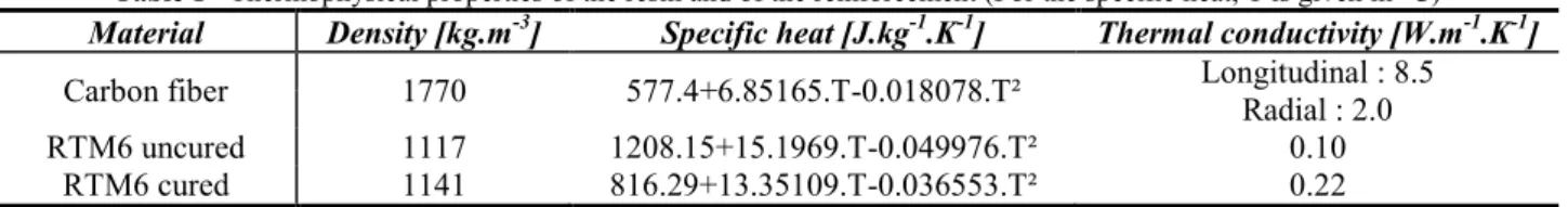
The materials considered in this study are representative of those used in the aeronautics industry. The reinforcement is a non-powdered 2x2 twill-weave carbon fiber fabric (G986 reference) provided by Brochier. The resin is an epoxy resin of the Hexcel Company (Ref. RTM6) whose thermal conductivity in liquid and solid states has been considered independent of temperature. DSC measurements were conducted to determine the specific heat of the reinforcement and of the resin in both states. Thermophysical properties are summarized in Table 1.

Table 1 · Thermophysical properties of the resin and of the reinforcement (For the specific heat, T is given in °C)

! "

Carbon fiber 1770 577.4+6.85165.T-0.018078.T² Longitudinal : 8.5 Radial : 2.0

RTM6 uncured 1117 1208.15+15.1969.T-0.049976.T² 0.10

RTM6 cured 1141 816.29+13.35109.T-0.036553.T² 0.22

All rights reserved. No part of contents of this paper may be reproduced or transmitted in any form or by any means without the written permission of TTP, www.ttp.net. (ID: 194.167.201.135-09/11/12,10:57:07)

(3)

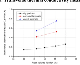
Figure 1 · Transverse thermal conductivities of dry preform, uncured laminate, and cured laminate for different fiber contents

3. Transverse thermal conductivity measurement

The composite sample is placed between the heating platen of a home-built press. Predefined thermal cycles are imposed on them, in order to obtain a 1D thermal gradient within the thickness of the part. The temperature evolution inside the preform is measured by three 80µm-diameter K-type thermocouples, that are disposed at different locations in the thickness of the part. Their exact positions are measured afterwards, using a binocular microscope. Carbon plies are surrounded by an insulating guard which limits the lateral thermal losses, and prevents the flow of the liquid resin under pressure. The estimation of the transverse thermal conductivities is performed by minimizing the squared difference between calculated and measured temperatures in the sample [1]. The identification method is based on the conjugate gradient algorithm coupled with an adjoint system. The measurements were carried out with balanced laminate [0 ° / 45 °] n / 2 , for different fiber volume fractions Vf. Four fiber volume fractions have

been tested in the case of the dry-preform, and two for uncured and cured laminates, as these experiments are a little more delicate to carry out. Figure 1 compares the transverse conductivity results of composites for all states of the resin.

4. In-plane thermal conductivity measurement

Whereas the measurement in the transverse direction is carried out conventionally, it is much more tricky in the planar direction, because heat transfer is more difficult to control in this direction. A special apparatus has been designed to impose the heat flux in the plane.

Experimental set-up · The experimental device is a small RTM mold made of Teflon® (PTFE). It

is composed of two symmetrical parts and allows the molding of square plates of 60 mm side and 10mm thick9 One half of this mold is depicted in Figure 3 and a cross-section view in Figure 4. This mold is placed between the heating platen of a press that allows temperature control to the prescribed initial temperature and also to apply the required closing pressure.

The temperature step is obtained by suddenly circulating a coolant fluid (oil in this study) inside a channel located at the edge of the sample, at a different temperature than the one of the mold. This channel is placed inside a copper insert, in order to reach a homogenous surface temperature. Moreover, since the mold is made of Teflon®, it is thermally more insulating than the carbon fiber and the composite. Therefore, during the step, heat transfer occurs mainly between the copper and the composite part. Due to the configuration of the insert (Figure 4), the step is applied on a small surface of the composite edge allowing to obtain rapidly and on a short distance a quasi uniform

Figure 3 · Half of the home-designed RTM-mold Figure 4 · Schematic view of a cross-section of the experimental mold

(4)

temperature through the thickness of the part. Thus, heat will diffuse preferentially in the plane of fibers. Moreover, the mold is surrounded by several centimeters of insulating material to reduce heat losses between the lateral faces of the mold and the ambient air.

The sample to characterize consists in two identical 5 mm thick preforms. 80µm K-type thermocouples are positioned in the direction of propagation of the thermal step (x-axis in Figure 3), at half-thickness of the preform and at equal distance from lateral sides. They are placed such as their wires are along isotherms. The distance between the thermocouples and the copper insert is accurately measured using a binocular microscope. The temperature of the copper insert is measured by a thermocouple TC0 fixed on its lower face (Figure 4). A vacuum pump connected to

the vent allows the injection of resin. A pressure regulator connected to the compressed air system ensures a low packing pressure (0.5 bar) after the end of the filling of the part to minimize residual porosity. The temperatures are recorded using Agilent HP34970A acquisition system.

A 3D-model of the device was first used to confirm that heat transfer mainly occurs in the cross-section of the mold. It appears that 3D effects cannot be neglected anymore after 700 seconds. In order to guarantee this assumption, the time interval used for the identification with the 2D model is limited to 500s. At steady-state, the composite sample is not isothermal. Indeed, the copper insert acts as heat sink and causes heat loss, and therefore a local cooling. The power of this heat sink is beforehand estimated to get an initial numerical thermal state as close as possible as the experimental one. In this study, the longitudinal conductivity (λx) and the thermal contact resistance

between the copper and the composite (Rt) must be estimated. The transverse conductivity is

obtained from the results of the transverse measurement (Figure 1). The sensitivity of the temperature to main parameters (ρCp, λx, λy and Rt) was calculated for the 5 thermocouples (TC1 to

TC5). This analysis aims firstly to highlight the relevance of the bench design for the estimation of

the unknown parameters, and secondly to determine the confidence intervals. We noticed that the sensitivities to thermal inertia ρCp are the most important, it is hence essential to determine accurately these parameters (Table 1). As expected, the sensitivity to the transverse conductivity λz

is significant only for the first thermocouple. However, this thermocouple must be kept because it allows determining the thermal contact resistance between the copper and the mold (Rt), since the

sensitivity of the latter is maximum for this thermocouple.

Identification method · To determine both parameters λx and Rt, a least squares criterion J is

defined by :

, = ~− (1)

where k is the thermocouple number and n the time step. T is the computed temperature and ~ the experimental one. The value of the L-S criterion depends on the two parameters to identify. The couple (λx, Rt) can easily be deduced from the minimum of this criterion.

Experimental protocol · A measurement cycle allows estimating for each composite part the

in-plane thermal conductivities of the dry preform, the composite at uncured and cured states. The cooling steps are carried out only when a steady-state is reached.

Table 2 · Main steps of a complete measurement cycle

Step Dry-preform Step Uncured laminate Step Cured laminate

1 Heating the mold at 130°C 4 Quasi-isothermal injection 7 Homogenization of the mold temperature

2 Measurement on the preform by

temperature step 5

Homogenization of the mold

temperature 8

Measurement on the cured composite by temperature

step

3 Preparing the injection (degassing

the resin, vacuum the preform)

6 Measurement on the liquid composite by temperature step

(5)

Three fiber volume fractions with balanced lay-ups were tested. A fourth sample validated the measurements reproducibility. Results are summed up in Table 3.

Table 3 · Configuration of the samples

Part Vf [vol %] Plies number (n) Reinforcement reference Lay-up

1 53.3 32 G986 [0°/45°]16

2 40 24 G986 [0°/45°]12

3 60 36 G986 [0°/45°]18

5. Modeling of thermal conductivity

The method used in this part is a two-step method that was developed by Kulkarny and Brady [2]. The first step consists in determining the transverse and longitudinal thermal conductivities of a single unidirectional lamina. In the second step, we consider the different orientations of fibers in the stacking sequence to obtain the laminate thermal conductivity tensor. We provide here a modified model [1] which adapts to the case of woven reinforcements.

Conductivity modeling of unidirectional composites: The starting material is a unidirectional

lamina, in which the fibers are all parallel to each other. The thermal conductivity parallel to the fiber direction, λ1, is easily obtained by the parallel model, or rule of mixtures [2, 3], by

= 1 − + ‖ ₍₂₎

where and denote respectively the volume fraction and the thermal conductivity of the resin, which is assumed to be isotropic, while ‖ stands for the corresponding property of the fibers, parallel to their longitudinal axis. Due to the difference between the in-plane and out of plane chemical bonds, graphite is a highly anisotropic material. While the conductivity in the basal planes is high, it is much lower through these planes. Therefore, there is a gap between the thermal conductivities in the longitudinal, ‖, and transverse direction, , of the fiber [3]. In this study, we will consider this anisotropy and use two values of fiber conductivity. The properties of standard modulus carbon fiber are presented in the following table.

Table 4 · Thermal conductivities of a standard modulus carbon fiber

Standard modulus carbon fiber (T300J)

Longitudinal thermal conductivity Radial thermal conductivity 8.5 W.m-1.K-1 [5] 2.0 W.m-1.K-1 [3]

In the transverse direction of the lamina (λ2), plenty of models attempt to predict the thermal

conductivity. Based on a potential analogy, Charles & Wilson and Maxwell models [2, 4, 6] were selected because they offer quite simple relationships describing the conductivity of randomly distributed and non-interacting discs in a homogenous matrix.

= 1 +_{1 −} +₊ 1 −_{1 +} = ! + 2 + 2 # − $_{+ 2 − # − $}% (3) (4)

where denotes the radial conductivity of a fiber. Assuming that the lamina is transversely isotropic, the relation λ2=λ3 applies, and the thermal properties can be finally described by only two

parameter, i.e. λ1 and λ2.

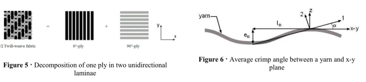
In-plane conductivity modeling of woven composites · In order to calculate in-plane thermal

conductivities, the woven reinforcement can be broken down into a sequence of unidirectional laminae. Thus, a twill-weave fabric made up of tows at 0° and 90° will be split into two unidirectional laminae, as shown in figure 5.

(6)

Figure 5 · Decomposition of one ply in two unidirectional

laminae

Figure 6 · Average crimp angle between a yarn and x-y

plane

We assume that all laminae are identical in thickness and in fiber fraction. Only the fiber orientation in each ply varies. Thermal contact resistance between the laminae, as interfacial defects (porosities, etc), are neglected. Global conductivity tensor (λx, λy, λz) of one ply can then be obtained

[2] through principal conductivities of an UD-lamina (λ1 and λ2) by:

,&= |cos +&| + |sin +&| .,&= |sin +&| + |cos +&| /= (5) (6) (7)

where θi represents the fiber orientation angle with respect to the global x-axis for the ply i. These

components for a single ply are used further to infer global thermal conductivity tensor components of the fabric composite. These are obtained by stacking N plies of the reinforcement and averaging their conductivities.

Transverse conductivity modeling · Fiber waviness is inherent in many reinforcing fabric, unlike

unidirectional composites, for which all fibers are nearly perpendicular to the z-axis. In fact, fiber crimping can be observed with woven reinforcements. In such situations, each fiber bends over or under another, so its axis departs from a straight line and follows a simple or complex wavy path. In this part, we take this effect into account and bring a correction to the previous estimated conductivities. These fabrics are characterized by a critic crimp angle αc which is the maximum

angle that takes a yarn with respect to the x-y plane. Average crimp angle is defined by: 0 = tan3 ₄56

768 (8)

where eα and lα are reinforcement-dependent lengths defined as shown in figure 6. Assuming that

all plies are most of the time identical in thickness, the effective transverse conductivity is then given by:

/= |sin 0| + |cos 0| (9)

We noticed that the effective longitudinal conductivity was not affected by the fiber crimp angle. Indeed, carbon fibers conduct heat much better than the resin, and fibers govern accordingly planar conductivity, especially since the value of the angle α is low.

6. Results & discussion

We used G986 fabric and assumed it was composed of standard modulus carbon fibers (T300J type). Considering that the matrix is air for the dry reinforcement, we will take into account the thermal conductivity of air at 130°C (λair=0.034W.m-1.K-1). By micrographic observations, we

calculated the crimp angle α in a cured laminate. Thus, we obtain 0 ≃ 1°. Thermal data are summarized Table 1.

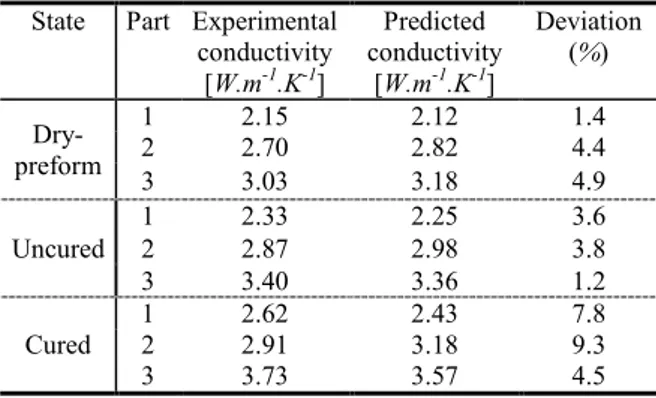
In-plane conductivity · The global conductivity seems to increase almost linearly with fiber

volume fraction (see Table 5). Satisfactory agreement is found between these models and experimental data for uncured and cured composites. The deviation generally does not exceed 5%, except for cured part, for which the deviation reaches more than 9%. It may be assumed measurement errors due to a problem of porosity or a bad fiber-matrix interface.

Transverse conductivity · On the whole, the comparison indicates good agreement between the

predicted transverse conductivity of the proposed models and our results, as shown in Figure 7. Unlike the in-plane case, both models are consistent, but not strictly equivalent. An excellent

(7)

Figure 7 · Comparison between calculated and measured

transverse conductivities for all states of composite

agreement is found for the dry-preform and the cured laminate, since our results are fitted between the two analytical models regardless of the fiber content. Moreover, it seems that the Maxwell model is more suitable for high fiber volume fractions, and that Charles & Wilson is more effective for lower fiber contents. Nevertheless, the uncured transverse conductivity deviates from

Table 5 · Comparison between calculated and measured

in-plane conductivities for all states of composite

the models by a maximum of 14%, which represents only about 0.06W.m-1.K-1. This difference can be explained by the uncertainty on the value of the conductivity of the raw resin, which has a relatively high sensitivity on the models. This may justify a new determination of this conductivity.

7. Conclusion

An experimental protocol was defined to measure in-plane and transverse conductivities of composite samples. The experimental bench developed for this study allows determining the values of the thermal conductivities in the planar direction. In comparison with other characterization devices, this one makes it possible to estimate the conductivities during the different stages of the molding: from the dry preform, to the raw composite and finally to the cured composite. The experimental bench and the identification program developed have provided satisfactory results. A perspective of this work will consist to identify simultaneously the in-plane and transverse conductivities and specific heat of the material by developing a new measurement apparatus and using a more effective identification. Charles & Wilson and Maxwell modified models provided a good agreement with the experimental data. The comparison with the experimental data revealed that they could be used to accurately predict the effective thermal conductivities of dry, liquid, and cured woven-reinforced composites.

References

[1] D. Lecointe, Caractérisation et simulation des processus de transferts lors d’injection de résine pour le procédé RTM, Ph. D. Thesis, Nantes University, 1999

[2] M. R. Kulkarni & R. P. Brady, Composites Science and Technology #$, A model of global thermal conductivity in laminated carbon-carbon composites, 1996

[3] R. Rolfes & U. Hammerschmidt, Composites Science and Technology #%, Transverse thermal conductivity of CFRP laminates: a numerical and experimental validation of approximation formulae, 1995

[4] R. Pal, Composites Part A &, On the Lewis-Nielsen model for thermal/electrical conductivity of composites, 2008

[5] B. N. Cox & G. Flanagan, National Aeronautics and Space Administration, Handbook of analytical methods for textile composites, 1997

[6] I. H. Tavman, Int. comm.. Heat and Mass Transfer, Vol 25, No. 5, pp 723-732, Effective thermal conductivity of isotropic polymer composites, 1998

State Part Experimental conductivity [W.m-1_.K-1_] Predicted conductivity [W.m-1_.K-1_] Deviation (%) Dry-preform 1 2.15 2.12 1.4 2 2.70 2.82 4.4 3 3.03 3.18 4.9 Uncured 1 2.33 2.25 3.6 2 2.87 2.98 3.8 3 3.40 3.36 1.2 Cured 1 2.62 2.43 7.8 2 2.91 3.18 9.3 3 3.73 3.57 4.5

1096 Material Forming ESAFORM 2012

Powered by TCPDF (www.tcpdf.org) Powered by TCPDF (www.tcpdf.org) Powered by TCPDF (www.tcpdf.org) Powered by TCPDF (www.tcpdf.org) Powered by TCPDF (www.tcpdf.org) Powered by TCPDF (www.tcpdf.org)