HAL Id: hal-00134548
https://hal.archives-ouvertes.fr/hal-00134548
Submitted on 5 Mar 2007HAL is a multi-disciplinary open access
archive for the deposit and dissemination of sci-entific research documents, whether they are pub-lished or not. The documents may come from
L’archive ouverte pluridisciplinaire HAL, est destinée au dépôt et à la diffusion de documents scientifiques de niveau recherche, publiés ou non, émanant des établissements d’enseignement et de
Presentation of KI-COF, a phenomenological model of
variable friction in fretting contact
Mohammed Cheikh, Stéphane Quilici, Georges Cailletaud
To cite this version:
Mohammed Cheikh, Stéphane Quilici, Georges Cailletaud. Presentation of KI-COF, a phenomeno-logical model of variable friction in fretting contact. Wear, Elsevier, 2007, 262 (7-8), pp.914-924. �10.1016/j.wear.2006.10.001�. �hal-00134548�
Presentation of KI-COF, a phenomenological
model of variable friction in fretting contact
M. Cheikh
1,
IUT de Figeac, avenue Nayrac F-46100 Figeac, France
S. Quilici G. Cailletaud
Centre des Mat`eriaux P.-M. Fourt, Ecole de Mines de Paris, UMR CNRS 7633, BP 87 F-91003 Evry, France.
Abstract
In this paper, a new phenomenological model, called KI-COF is developed to ac-count for variable coefficient of friction (COF) in space and time. The COF is no longer considered as a global value valid for the whole contact area. A local value is introduced instead, the evolution of which is governed by the local history of the contact and the amount of slip.
Key words: Fretting wear, fretting fatigue, variable friction, coefficient of friction, contact.
1 INTRODUCTION
Fretting is the consequence of low oscillations between two bodies in contact [1]. The cycles can result from small relative displacements or stress variations in the bodies. It is most commonly found in all kinds of press fits, spline con-nections, leaf springs, riveted and bolted joints, nuclear fuel elements and also in wire ropes. The most significant factor in a contact with fretting is the coef-ficient of friction [2]. This factor is influenced by the surface quality, the wear induced by the fretting, the behavior of the third body, etc. Many studies have been completed for characterizing friction in fretting tests [2]. In the numerical studies dealing with fretting, the COF is generally presented as a constant of
1
Corresponding author. E-mail: mcheikh@univ-tlse2.fr; Fax: +33 5 65 50 30 61. Other address: Centre CROMeP, EMAC, Campus Jarlard - 81013 ALBI C´edex.
the contact [3,4]. Actually, the COF varies according to the modification of the surface quality and the lubricant and it is never constant [5].
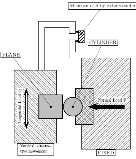
The present study is performed in connection with experiments made at ‘Lab-oratoire de Tribologie et Dynamique des syst`emes (LTDS)’ of ‘Ecole Centrale de Lyon’ [6,7] for characterizing the fretting behavior of a titanium alloy. Fig-ure (1) presents the experimental apparatus used by Fridrici et al. [6]. It is composed of a cylinder, subjected to a normal load P, sliding on a plane. The displacement amplitude δ is applied to the plane. In this test, the cylinder is coated and lubricated, the plane is shot peened without specific coating. Figure (2) shows a typical evolution of the COF during a fretting test with a displacement amplitude of δ∗ = 50µm. Each cycle of fretting represents the
evolution of the ratio Q/P according to displacement amplitude δ with Q the tangential force. The COF µ is identified in the phase corresponding to the gross slip. By choosing the law of Coulomb |Q|/P <= µ, the horizontal sides of these cycles represent the evolution of the COF µ = |Q|/P according to displacement amplitude δ. The near-vertical sides of the friction loops corre-spond to the sticking behavior. These sides are not completely vertical due to the flexibility of the plane-cylinder set. The slope of these sides corresponds to the rigidity of the contact between the plane and the cylinder.
This figure shows well that the coefficient of friction is variable in the interior of the cycles. It evolves with the amplitude and the direction of the slip. The COF also evolves with time while the fretting cycles number increases. The cycles have a parallelogram shape with horizontal sides for the first cycles. With the evolution of the fretting, these sides become oblique. The first cycles can be modeled with a constant µ. The cycles with oblique sides cannot be modeled with a constant COF. To solve this problem, the numerical studies classically model this evolution by carrying out several calculations with different COF [8,9]. There is an absence of a friction model that can accurately simulate this temporal and spatial variations of the COF during fretting contact.
In this paper, a new phenomenological model, called KI-COF (Kinematic Isotropic coefficient Of Friction) is developed to account variable COF in space and time. The COF is no longer considered as a global value valid for the whole contact area. A local value is introduced instead, which evolution is governed by the local history of the contact and the amount of slip. The framework is inspired from elastoplasticity. The model presented in this study will allow us to derive a full modeling of the friction history during the whole life of the contact. The evolution of the COF depends on two variables: an isotropic evolution related to accumulated slip and a kinematic component computed from the actual relative position of the bodies. Other authors have already proposed an elastoplastic framework [10,11], nevertheless, to the best knowl-edge of the authors, the combination of an isotropic and a kinematic variable is original.
Section 2 presents the elementary components of the friction model. Section 3 shows the finite element implementation of this model in the computer code Z´eBuloN[12]. The last section presents the fretting cycles obtained by this model compared to those obtained by experiment in the case of cylinder-plane problem.
2 DESCRIPTION OF THE MODEL
In fretting contact, the increase of the roughness of contact surfaces with time is accompanied by a continuous evolution of the COF. This evolution is independent of the slip direction inside the cycles. This evolution represents the isotropic component of the COF. An evolution of µ versus slip is also found inside the cycles. The increase of slip is accompanied by an increase of the COF and the opposite slip is always facilitated compared to the current slip. This represents the kinematic component of the evolution of the COF. The kinematic evolution is the result of the degradation of the contact by abrasive wears, by the modification of the form of the contact surface, by the behavior of the third body, etc. The following section presents the evolution model of the isotropic and kinematic components of the COF.
2.1 Modeling of the isotropic COF
The isotropic COF µR represents the expansion which the cycle of fretting
undergoes with time. Between two cycles of fretting, µR can be represented
by the variation of the initial COF µ0 between these two cycles. For example,
in figure (3), µR1 represents the value of the isotropic component of the COF
µR after the first cycle. The isotropic COF is independent of the current slip
direction δ, it can thus be parameterized by a scalar variable like the energy of slip Ed or the accumulated slip δ.
In this study we chose to model the isotropic COF µR according to
accumu-lated slip µR = f (δ). Figure 4 presents some examples of the evolution of µR
according to accumulated slip. To model the experimental results of µ, the function f must have a nonlinear form in δ and must have a threshold of saturation. The following form is used:
µR = µ1(1 − exp(−bRδ)), (1)
with µ1 and bR the parameters of the used material. The coefficient µ1
factor of acceleration of the isotropic evolution of the COF. The accumulated slip is defined by δ(t) = t Z 0 | ˙δ|dτ (2)
with ˙δ the speed of the slip. Figure (4) presents the µR obtained by this model
with the experimental results.
2.2 Modeling of the kinematic COF
As mentioned above, the kinematic COF represents the component of the evolution of the COF dependent on the current slip δ. For low values of µ the slip is generally full and the cycles have the shape of a parallelogram. Before the COF does not reach significant values, so that the slip is transformed into partial slip, the kinematic COF is linear in δ hence: µX = Hδ. For example, in
the right curve of figure 3, µX1represents the value of the kinematic COF µXat
the end of the first alternation of the first cycle. The modulus H represents the slope of slip. This modulus is generally variable and depends on accumulated slip δ that is H = g(δ). The function g represents the upward evolution of the slope in the phase of slip. If the modulus H is constant, our model will be similar to the plastic model of Prager.
The experimental results show that the function g must have a nonlinear form function of δ and must have an asymptotic value after the saturation of the COF evolution. The function g is modeled by:
g(δ) = µ′
2(1 − exp(−bXδ)β), (3)
with bXand β the constants of fretting of the selected material. These two
coef-ficients allow to adjust the acceleration of the kinematic evolution of the COF. The coefficient µ′
2 represents the slope value after saturation of evolution. This
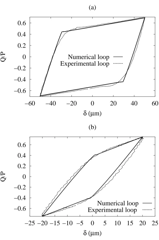
coefficient is not constant and depends on the maximum displacement ampli-tude of the test. Figure 5 presents two cycles obtained after saturation in two tests with displacement amplitudes of δ∗ = 50µm and δ∗ = 20µm, for the first
and the second test, respectively. The saturation slope for the first test is less significant than that of the second test with smaller displacement amplitude. This difference is explained by the fact that a small displacement amplitude is more favorable to the formation of a pad, which impedes slip and produces a sharp-pointed form of the cycle of fretting. This difference is also explained by the importance of the role of the displacement amplitude in the behavior
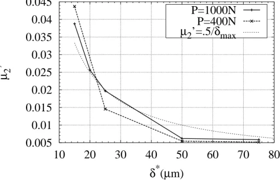
of the third body in a contact with fretting. The slope at saturation evolves in the form of a reverse function µ′
2 = µ2/δmax (see figure 6).
The kinematic COF takes then the following form: µX=
µ2
δmax
(1 − exp(−bXδ)β)δ. (4)
with δmaxrepresents the value of the displacement amplitude at the end of the
alternation of the cycles. At the beginning of the slip for any alternation and at each change of the direction of slide, the kinematic COF µX goes back to
zero. For example, in figure 3, at the points A and B, the value of µX is nil.
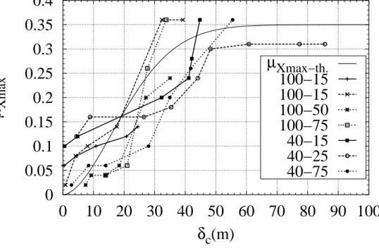
Figure (7) represents some examples of evolution of µXmax= µ2
h
1 − exp(−bXδ)β
i
(5) obtained by experiment and by the used model. µXmax represents the value of
µX at the end of the alternation of each cycle hence when δ = δmax.
2.3 Modeling of the total COF
The total COF µ is finally the sum of the kinematic component, the isotropic component and the initial COF µ0:
µ = µ0+ µ1 h 1 − exp(−bRδ) i + µ2 δmax h 1 − exp(−bXδ) i δ (6)
It is a model with 6 coefficients whose values depend on selected material. With this model, Coulomb law is introduced, so that:
|Q| <= µP, (7)
if |Q| < µP stick, (8)
if |Q| = µP slip. (9)
By choosing the variables Qy = µ0P , QR = µRP and QX = µXP , the law of
Coulomb (7) takes the form of a yield function:
f (Q, QX, QR) = |Q − QX| − Qy − QR, (10)
if f < 0 stick, (11)
if f = 0 slip. (12)
The KI-COF model (6) is general and can have simpler forms according to the conditions of fretting. The evolution of the COF depends on the coating and the lubricant. In the case of a coated and lubricated set, the evolution of the COF is progressive under the effect of the coating and the lubricant. The progressive damage of the lubricant is accompanied by a progressive increase in the COF. In this case the general form of the model (6) can be used. In the case of a cylinder without coating, the COF has a more significant value and almost constant along the test. In this case there is no isotropic evolution of the COF and the function g (Eq. 3) is constant. Kinematic evolution depends only on the slip δ. The model (6) takes a simpler form:
µ = Hδ (13)
similar to the linear kinematic model of Prager. The constant modulus H represents the straight curve slope in the slip phase of the fretting cycle. In this case the cycles of fretting take the form of the right cycle of figure 3.
3 NUMERICAL IMPLEMENTATION
This model applies locally in the contact area. In a finite element computation, for example, each element has its COF dependent on history, state of stress, slip, status of the contact zone, etc. This section describes the implementation of this model in the FE code Z´eBuloN. To model the contact, Z´eBuloN uses an impactor and a target. The impactor is composed of a set of nodes whereas the target is made up of a set of lines (or a set of faces for the 3D case). An element of contact is composed by a particle (a candidate node of the
impactor) and the target. The initial COF µ0 and the other 5 constants of
the model are global characteristics of the contact area. Each element of the contact zone inherits (in the meaning of object oriented programming) the same values of these constants. On the other hand, each element of contact has its accumulated slip δ and its current slip δ. Each element has thus, its kinematic component and its isotropic component of the COF.
3.1 Identification of the model
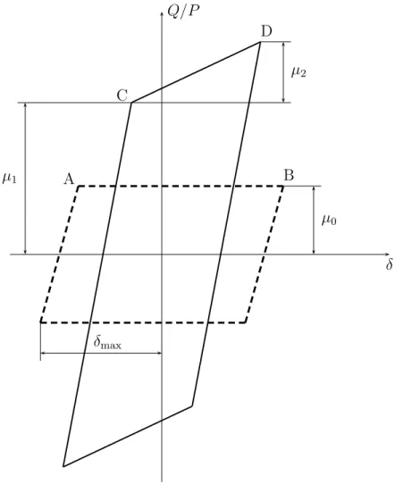
Figure (8) represents the identification method of the coefficients of the model. The coefficient µ0 is identified at the first cycle. It corresponds to the value
of Q/P at the point A or B. The coefficient µ1 is identified at the saturation
cycle. It corresponds to the Q/P value at the point C of the saturation cycle. The coefficient µ2 is identified at the point D. It corresponds to the slope of
saturation cycles. The coefficient δmax corresponds to the half alternation of
the cycles.
The coefficient bR represents the isotropic evolution which corresponds to the
evolution between the points A and C in the figure. In the same way, bX with
β, represent the kinematic evolution which corresponds to the evolution from the point B to D in the figure. The identification in fretting of a material is carried out after a large number of cycles which can reach the million. In order to simulate numerically these tests with an acceptable computing time, an acceleration factor of the coefficients evolution of the model is used. In model (6) one replaces the coefficients bR and bX by respectively b′R and b′X
with: b′
R = abR and b′X= abX (14)
The coefficient a is the acceleration factor of the model.
A second possible technique to accelerate calculation is the technique of cycle skip. Instead of modifying the coefficients bR and bX, one increments
periodi-cally the value of accumulated slip. The coefficient a in this technique repre-sents the value of increment of the jump of cycle. Considering the weakness of displacement amplitude in front of accumulated slip, the two techniques are equivalent. In the applications presented thereafter the technique of accelera-tion is used.
3.2 The contact algorithm
To deal with the problems of contact Z´eBuloN uses a direct method known as method of flexibility [13,14,15,16]. With this method the conditions of contact are not introduced explicitly into the variational formulation of the problem. The reactions of contact are calculated a priori, then added in the equilibrium equations as known additional external forces in the deformed configuration Ct+∆t. The residual is then defined at time t + ∆t as:
Rt+∆t = Fintt+∆t+ F t+∆t
ext + R
t+∆t
c = 0, (15)
Displacements uc due to the contact are related to the contact reactions rc on
a local frame of the element of contact by the relation
uc= TTK−1T rc= W rc (16)
with W = TTK−1T r
c the matrix of flexibility condensed on the scale of the
contact. The matrix T is a linear operator allowing to express the local vari-ables in the global frame such as Rc = T rc. The system (16) represents the
equilibrium system of the structure subjected to the contact reactions only. In order to define displacements uc and the reactions rc, the law of Coulomb
7 and the condition of impenetrability (Signorini condition) are imposed. Signorini condition is expressed by rn= ProjIR+(rn− ρnxn) where ProjIR+
de-notes the orthogonal projection on the positive real set IR+; ρn> 0 and xnthe
gap between the particle and the target. The law of Coulomb can be expressed by: rt = ProjC(rt− ρtδ) where C is the disk {rt∈ IR2 : krtk ≤ µrn} and ρt> 0
[17]. To define the local unknown factors (uc, rc) the following system is solved:
W rc= uc
rn= ProjIR+(rn− ρnxn), ρn > 0
rt= ProjC(rt− ρtδ), ρt> 0 (17)
δ = δlib+ uct
xn= xlibn+ ucn+ x0n
with xlibn and δlibrespectively the gap and free slide when no contact reactions
are applied and x0
nis the initial altitude of the particles. Once defined the local
contact reactions rc, one computes the global contact reactions Rc = T rc and
solves the system (15).
4 APPLICATION
In order to validate the model, an application on the case of a cylinder-plane contact and a comparison with the experimental results of the LTDS are pre-sented thereafter.
4.1 Mesh and boundary conditions
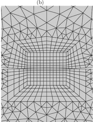
Figures (9) and (10) represent the mesh of the system. The influence of the size of the mesh on the developed model is checked by using two meshes (see figure 10): A coarse mesh with a typical element size of 50µm × 25µm on the
level of the contact, that is 1/10 of the total contact area. And a finer mesh characterized by elements of 8µm × 4µm in the contact area, that is about 1/64 of the total contact area. First mesh allows a fast calculation of the cycles of fretting, whereas the second provides, in addition to the simulation of the cycles, a finer estimation of the local variables like stresses and strain in the contact area. This mesh is discreted with 1050 elements 2D with linear interpolation and 761 nodes, hence 1522 DOFs for the problem. For the second mesh, the set is discreted with 4744 elements 2D with linear interpolation and 3796 nodes, hence 7592 DOFs for the problem.
In experiments, at the beginning of each test, a vertical load P is applied. The test is then continued by applying a cyclic displacement, with an amplitude of ±δ∗ to the plane (see figure 11). The normal load is applied to the cylinder in
the form of an imposed displacement in order to reproduce the desired loading. This way of imposing the loading is in conformity with the tests performed at LTDS. In these tests, the imposed loading is not controlled and its value can vary during the test. The ends of the plane are constrained along the axis y. The displacement amplitude δ(t) is applied to the plane along the x axis. The higher extremity of the cylinder is constrained along the x axis.
With the KI-COF model, it is not necessary to model the coating and/or the lubricant. The presence of the lubricant and the evolution of the contact with coating are taken into account indirectly by the evolution of the isotropic and kinematic hardening. In this study, the coating and lubricant are not represented.
Due to the small size of the contact area in front of the transverse dimension of the set, the mechanical behavior is supposed to be in plane deformation. A viscoplastic model with non linear isotropic and kinematic hardening is used [18].
4.2 Results
In order to show the sensitivity of the KI-COF model to the smoothness of the mesh, all calculations were carried out by the two meshes presented on figure (10). The results of the calculations obtained by the two meshes are identical. Figure (12) represents a sample of fretting cycle obtained by the two meshes for
a displacement amplitude δ∗ = 20µm and a loading P = 1000N. This figure
shows well that the results of the two meshes are similar. In the following results the coarse mesh is used. Figure (13) presents the local evolution of the slip according to the cycles and the position x of the contact nodes on the level of the interface cylinder-plane. This figure shows a fall of local slip with the cycles of fretting. The opposite phenomenon is observed on figure (14), with
the evolution of the cycles the accumulated slip δ increases. This increase of the accumulated slip is accompanied by an increase in the COF value as figure (15) shows it. Figures 13, 14 and 15 show for each cycle, in particular for the last cycles, that the local slip, the accumulated slip and the COF µ are more significant at the end of the cylinder-plane interface than in the medium one. Figures 16-18 present a sample of fretting test simulated by the suggested model with the coarse mesh in comparison with the corresponding experi-mental results. Figure 16 presents the results for a displacement amplitude
δ∗ = 20µm and a loading P = 1000N. For the loading P = 400N, figures
(17) and (18) present the results with displacement amplitude δ∗ = 25µm and
δ = 50µm respectively. The cycles with a legend LN represent the numerical cycles. The cycles with a legend LE represent the experimental cycles. For the experimental cycles the unit K represents 1000 cycles. In each figure, the fret-ting log is presented with some samples of cycles represenfret-ting the evolution of the COF according to time. Figure (16) shows that for the displacement amplitude δ∗ = 20µm, the slip regime is mixed. The shape of the log is
rect-angular in the beginning which is the characteristic of gross slip, and at the end of the test the shape of the log becomes elliptic which is the characteristic of partial slip. Cycles presented in this figure show the same evolution for the experimental and simulated results. In this figure, until the 325000th cycle, the cycles are parallelepipedic with sharp-pointed form at the end. After this cycle, the cycles become elliptic and the slip regime is partial. For the load P = 400N, the slip regime is gross for the displacement amplitude δ∗ = 25 and
δ∗ = 50 as figures (17) and (18) show it. The fretting logs have parallelepipedic
shape and the cycles keep a rectangular form along the test.
All the results presented in these figures demonstrate an acceptable agreement between the simulated evolution and the experimental cycles. The discrepan-cies between simulation and the experiment are due to the scatter in the ex-perimental results as shown in figures (4 and 7), and pointed out by Friedrich [7] .
5 Conclusion
In this paper, we proposed a model of evolution of coefficient of friction in fretting contact. This model was implemented in a finite element code. A constitutive equation is defined to predict the evolution of the coefficient of friction. The proposed rule, called the KI-COF model, introduces both an isotropic evolution and a kinematic evolution if the COF. Using this model, the COF is no longer uniform: in a FE computation, one defines a field of COF, which depends on each point of the local history of the contact. The agreement between the numerical simulations and the experimental results is
encouraging. The generalization of the model to the 3D case requires the use of an anisotropic model of friction: the kinematic variable will become a tensor, meanwhile the isotropic one will remain scalar.
Acknowledgments
This study is financially supported by SNECMA Moteurs. The authors wish to thank P. Perruchaut and S. Mosset (from SNECMA Moteurs-Villaroche) for the helpful discussion and permission to publish. The authors are grateful to V. Fridrici and S. Fouvry (from LTDS, Ecole Centrale DE Lyon) for providing experimental data and for fruitful discussions.
References
[1] R. B. Waterhouse. Fretting fatigue. Inter. Materials Reviews, 37(2):77–97, 1992.
[2] M. P. Szolwinski and T. N. Farris. An experimental study of fretting fatigue crack nucleation in airframe alloys: a life prediction and maintenance perspective. In Proceedings of 1st joint DoD/FAA/NASA conference on aging airfact, Ogden, UT, 1997.
[3] N. Str˝omberg. A Newton method for three-dimensional fretting problems. Int. J. Solids and Structures, 36:2075–2090, 1999.
[4] C. Petiot, L. Vincent, K. Dang Van, N. Maouche, J. Foulquier, and B. Journet. An analysis of fretting-fatigue failure combined with numerical calculations to predict crack nucleation. Wear, 181-183:101–111, 1995.
[5] D. R. Swalla and R. W. Neu. Influence of coefficient of friction on fretting fatigue crack nucluation prediction. Tribology international, 34:493–503, 2001. [6] V. Fridrici, S. Fouvry, and P. Kapsa. Effect of shot peening on the fretting wear
of Ti-6Al-4V. Wear, 250:642–649, 2001.
[7] V. Fridrici. Etude du comportement en fretting d’un alliage de titane Ti-6Al-4v: Application au dimensionnement du contact aubedisque de fan. Th`ese d’universit´e, ´Ecole Centrale de Lyon, 2002.
[8] A. E. Giannakopoulos and S. Suresh. A three-dimesional analysis of fretting fatigue. Acta mater., 46(1):177–192, 1997.
[9] C. T. Tsai and S. Mall. Elasto-plastic finite element analysis of fretting stresses in pre-stressed stip in contact with cylindrical pad. Finite elements in analysis and design, 36:171–187, 2000.
[10] A. Curnier. A theory of friction. Int. J. Solids Structures, 20(7):637–647, 1983. [11] R. Michalowski and Z. Mroz. Associated and non-associated sliding rules in
contact friction problems. Arch. Mech., 30:259–276, 1978.
[12] Zebulon. A finit element code. See www.nwumerics.com for more information. [13] A. Francavilla and O. C. Zienkiewicz. A note on numerical computation of
elastic contact problems. Int. J. Numer. Methods Eng., 9(4):913–924, 1975. [14] T. D. Sachdeva and C. V. Ramakrishnan. A finite element solution for the
two-dimensional elastic contact problems with frictions. Int. J. Numer. Methods Eng., 17:1257–1271, 1981.
[15] M. Jean and G. Touzot. Implementation of unilateral contact and dry friction in computer codes dealing with large deformations problems. Journal de M´ecanique th´eorique et appliqu´ee, 7(supplement n: 1):145–160, 1988.
[16] M. Wronski. Couplage du contact et du frottement avec la m´ecanique non lin´eaire des solides en grandes d´eformations. Th`ese d’universit´e, Universit´e de Technologie de Compi`egne, 1994.
[17] F. Jourdan, P. Alart, and M. Jean. A gauss-seidel like algorithm to solve frictional contact problems. Computer Methods in Applied Mechanics and Engineering, 155:31–47, 1998.
[18] J. Lemaitre and J.-L. Chaboche. M´ecanique des mat´eriaux solides. Dunod, Paris, 1988. 2e´edition.
−0.6
−0.4
−0.2
0
0.2
0.4
0.6
−60 −40 −20
0
20
40
60
80 100 120
Q/P
δ (µ
m)
Loops
10k
50k
75k
100k
130k
150k
200k
500k
Figure 2. Examples of fretting cycles for δ∗ = 50µm. The unit k represents 1000
µR1 δ Q/P µX1 δ A B Q/P
Figure 3. Definition of the kinematic component and the isotropic component of the COF. The left curve represents the isotropic evolution only (the kinematic evolution is neglected) and the right curve represents the kinematic evolution only (the isotropic evolution is neglected).
0
0.05
0.1
0.15
0.2
0.25
0.3
0.35
0
10
20
30
40
50
60
70
80
µ
Rδ
c(m)
µ
R−th100−15
100−25
100−50
100−75
40−15
40−75
Figure 4. Examples of evolution of the isotropic component of the COF µRaccording
to the accumulated slip δc = δ (in meters) obtained by the experiment. The first
number of every legend represents the loading, the second represents the imposed displacement. µR−th represents the evolution of µR obtained by our model (Eq. 1)
−0.6
−0.4
−0.2
0
0.2
0.4
0.6
−60
−40
−20
0
20
40
60
Q/P
δ (µ
m)
(a)
Numerical loop
Experimental loop
−0.6
−0.4
−0.2
0
0.2
0.4
0.6
−25 −20 −15 −10 −5
0
5
10 15 20 25
Q/P
δ (µ
m)
(b)
Numerical loop
Experimental loop
Figure 5. The displacement amplitude influence on the slope form of the saturation cycle: The slope of the cycle with δ∗= 20µm (case b) is more pronounced than the
0.005
0.01
0.015
0.02
0.025
0.03
0.035
0.04
0.045
10
20
30
40
50
60
70
80
µ
2’
δ
*(
µ
m)
P=1000N
P=400N
µ
2’=.5/
δ
maxFigure 6. Evolution of the slope after saturation for the loadings P=1000N and P=400N and for the theoretical value with µ2=0.5.
0
0.05
0.1
0.15
0.2
0.25
0.3
0.35
0.4
0
10 20 30 40 50 60 70 80 90 100
µ
Xmaxδ
c(m)
µ
Xmax−th.100−15
100−15
100−50
100−75
40−15
40−25
40−75
Figure 7. Examples of evolution of µXmax according to the accumulated slip δc= δ
(in meters) obtained by experiment. The first number of every legend represents the loading, the second represents the imposed displacement. µX−th represents the evolution of µXmax obtained by our model (Eq. 5)
C µ1 D µ2 A B µ0 δmax δ Q/P
Figure 8. Identification of the different coefficients of the model. The dashed cycle represents the first cycle and the other cycle represents the saturation one.
x y
z
(a) (b) x y z x y z
t P
t δ
−0.4 −0.2 0 0.2 0.4 −20 −15 −10 −5 0 5 10 15 20 Q/P δ (µm) coarse mesh finer mesh
Figure 12. Comparison between the cycles obtained by the fine mesh and the coarse mesh.
16 18 20 22 24 26 28 30 32 34 isoline of δ (µm) δ(µm) 32 30 28 26 24 22 20 18 0 200 400 600 800 1000 1200 1400 1600 1800 2000 Cycle number -0.3 -0.2 -0.1 0 0.1 0.2 0.3 x(mm) 16 18 20 22 24 26 28 30 32 34δ (µm)
Figure 13. Evolution of the local slip δ function of the number of cycles and the position x of the interface contact nodes.
0 10 20 30 40 50 60 70 80 90 isoline of δc (m) δc(m) 80 70 60 50 40 30 20 10 0 200 400 600 800 1000 1200 1400 1600 1800 2000 Cycle Number -0.3 -0.2 -0.1 0 0.1 0.2 0.3 x(mm) 0 10 20 30 40 50 60 70 80 90 δc(m)
Figure 14. Evolution of the accumulated slip δc = δ function of the number of cycles
0.2 0.25 0.3 0.35 0.4 0.45 0.5 0.55 0.6 0.65 0.7 0 200 400 600 800 1000 1200 1400 1600 1800 2000-0.3 -0.2 -0.1 0 0.1 0.2 0.3 0.2 0.25 0.3 0.35 0.4 0.45 0.5 0.55 0.6 0.65 0.7 µ isoline of µ (µ) 0.65 0.6 0.55 0.5 0.45 0.4 0.35 0.3 0.25 Cycles x(mm) µ
Figure 15. Evolution of the COF, function of the number of cycles and the position x of the interface contact nodes.
0 100 200 300 400 -20 -10 0 10 20 -0.5 0 0.5 -0.5 0 −0.6 −0.5 −0.4 −0.3 −0.2 −0.1 0 0.1 0.2 0.3 0.4 0.5 0.6 −25 −20 −15 −10 −5 0 5 10 15 20 25 Q/P δ (µm) NL 400 EL 400K −0.5 −0.4 −0.3 −0.2 −0.1 0 0.1 0.2 0.3 0.4 0.5 −25 −20 −15 −10 −5 0 5 10 15 20 25 Q/P δ (µm) NL 375 EL 375K −0.5 −0.4 −0.3 −0.2 −0.1 0 0.1 0.2 0.3 0.4 0.5 −25 −20 −15 −10 −5 0 5 10 15 20 25 Q/P δ (µm) NL 350 EL 350K −0.5 −0.4 −0.3 −0.2 −0.1 0 0.1 0.2 0.3 0.4 0.5 −25 −20 −15 −10 −5 0 5 10 15 20 25 Q/P δ (µm) NL 325 EL 325K −0.5 −0.4 −0.3 −0.2 −0.1 0 0.1 0.2 0.3 0.4 0.5 −25 −20 −15 −10 −5 0 5 10 15 20 25 Q/P δ (µm) NL 300 EL 300K −0.2 −0.1 0 0.1 0.2 −25 −20 −15 −10 −5 0 5 10 15 20 25 Q/P δ (µm) NL 10 EL 10K
Figure 16. Numerical and experimental cycles evolution for P = 1000N and δ∗= 20µm.
0 100 200 300 -50 -25 0 25 50 -0.5 0 0.5 -0.5 0 −0.9 −0.8 −0.7 −0.6 −0.5 −0.4 −0.3 −0.2 −0.10 0.1 0.2 0.3 0.4 0.5 0.6 0.7 0.8 0.9 −30 −20 −10 0 10 20 30 Q/P δ (µm) NL 1000 EL 1000K −0.9 −0.8 −0.7 −0.6 −0.5 −0.4 −0.3 −0.2 −0.10 0.1 0.2 0.3 0.4 0.5 0.6 0.7 0.8 0.9 −30 −20 −10 0 10 20 30 Q/P δ (µm) NL 900 EL 900K −0.9 −0.8 −0.7 −0.6 −0.5 −0.4 −0.3 −0.2 −0.10 0.1 0.2 0.3 0.4 0.5 0.6 0.7 0.8 0.9 −30 −20 −10 0 10 20 30 Q/P δ (µm) NL 700 EL 700K −0.8 −0.7 −0.6 −0.5 −0.4 −0.3 −0.2 −0.10 0.1 0.2 0.3 0.4 0.5 0.6 0.7 0.8 −30 −20 −10 0 10 20 30 Q/P δ (µm) NL 550 EL 550K −0.8 −0.7 −0.6 −0.5 −0.4 −0.3 −0.2 −0.10 0.1 0.2 0.3 0.4 0.5 0.6 0.7 0.8 −30 −20 −10 0 10 20 30 Q/P δ (µm) NL 500 EL 500K −0.5 −0.4 −0.3 −0.2 −0.1 0 0.1 0.2 0.3 0.4 0.5 −30 −20 −10 0 10 20 30 Q/P δ (µm) NL 100 EL 100K
Figure 17. Numerical and experimental cycles evolution for P = 400N and δ∗ = 25µm.
0 100 200 300 400 -50 -25 0 25 50 -0.5 0 0.5 -0.5 0 −0.8 −0.7 −0.6 −0.5 −0.4 −0.3 −0.2 −0.1 0 0.1 0.2 0.3 0.4 0.5 0.6 0.7 0.8 −60 −40 −20 0 20 40 60 Q/P δ (µm) CN 200 CE 200K −0.7 −0.6 −0.5 −0.4 −0.3 −0.2 −0.1 0 0.1 0.2 0.3 0.4 0.5 0.6 0.7 −60 −40 −20 0 20 40 60 Q/P δ (µm) CN 150 CE 150K −0.6 −0.5 −0.4 −0.3 −0.2 −0.1 0 0.1 0.2 0.3 0.4 0.5 0.6 −60 −40 −20 0 20 40 60 Q/P δ (µm) CN 120 CE 120K −0.6 −0.5 −0.4 −0.3 −0.2 −0.1 0 0.1 0.2 0.3 0.4 0.5 0.6 −60 −40 −20 0 20 40 60 Q/P δ (µm) CN 100 CE 100K −0.3 −0.2 −0.1 0 0.1 0.2 0.3 −60 −40 −20 0 20 40 60 Q/P δ (µm) CN 30 CE 50K −0.3 −0.2 −0.1 0 0.1 0.2 0.3 −60 −40 −20 0 20 40 60 Q/P δ (µm) CN 10 CE 10K
Figure 18. Numerical and experimental cycles evolution for P = 400N and δ∗ = 50µm.
![Figure 2. Examples of fretting cycles for δ ∗ = 50µm. The unit k represents 1000 cycles [7].](https://thumb-eu.123doks.com/thumbv2/123doknet/11616767.303874/15.892.158.707.329.722/figure-examples-fretting-cycles-µm-unit-represents-cycles.webp)