HAL Id: hal-01515084
https://hal.archives-ouvertes.fr/hal-01515084
Submitted on 27 Apr 2017HAL is a multi-disciplinary open access archive for the deposit and dissemination of sci-entific research documents, whether they are pub-lished or not. The documents may come from teaching and research institutions in France or
L’archive ouverte pluridisciplinaire HAL, est destinée au dépôt et à la diffusion de documents scientifiques de niveau recherche, publiés ou non, émanant des établissements d’enseignement et de recherche français ou étrangers, des laboratoires
Numerical Tools for the Control of the Unsteady
Heating of an Airfoil
Françoise Masson, Francisco Chinesta, Adrien Leygue, Chady Ghnatios, Elías
Cueto, Laurent Dala, Craig Law
To cite this version:
Françoise Masson, Francisco Chinesta, Adrien Leygue, Chady Ghnatios, Elías Cueto, et al.. Numerical Tools for the Control of the Unsteady Heating of an Airfoil. Journal of Mechanics Engineering and Automation, David Publishing, 2013, 3 (6), pp.339-351. �hal-01515084�
Numerical Tools for the Control of the Unsteady Heating
of an Airfoil
Françoise Masson1, 4, Francisco Chinesta1, 2, Adrien Leygue1, Chady Ghnatios1, Elias Cueto3, Laurent Dala4 and Craig Law4
1. EADS Corporate Foundation International Chair, GEM UMR CNRS - Ecole Centrale Nantes, F-44321 Nantes Cedex 3, France 2. Institut Universitaire de France,Paris 75 000, France
3. Aragon Institute of Engineering Research – I3A, Universidad de Zaragoza, Zaragoza E-50018, Spain
4. School of Mechanical, Industrial and Aeronautical Engineering, University of the Witwatersrand, Johannesburg 2000, South Africa
Abstract: This paper concerns the real time control of the boundary layer on an aircraft wing. This new approach consists in heating the surface in an unsteady regime using electrically resistant strips embedded in the wing skin. The control of the boundary layer’s separation and transition point will provide a reduction in friction drag, and hence a reduction in fuel consumption. This new method consists in applying the required thermal power in the different strips in order to ensure the desired temperatures on the aircraft wing. We also have to determine the optimum size of these strips (length, width and distance between two strips). This implies finding the best mathematical model corresponding to the physics enabling us to facilitate the calculation for any type of material used for the wings. Secondly, the heating being unsteady, and, as during a flight the flow conditions or the ambient temperatures vary, the thermal power needed changes and must be chosen as fast as possible in order to ensure optimal operating conditions.
Key words: Model reduction, PGD (proper generalized decomposition), heating of an airfoil, boundary layers, laminar-turbulent transition and separation point, friction drag, unsteady heating.
1. Introduction
A new proposal enabling us to control the boundary layer flow over an airfoil is under way [1]. It would influence the boundary layer’s laminar-turbulent transition and separation point, allowing an improvement in economic efficiency and safety of airplanes. This new approach proposed is associated with the unsteady surface heating regime using electrically resistant strips embedded in the wing skin. The control of the boundary layer’s separation and transition point will provide a reduction in friction drag, and hence a reduction in fuel consumption. The implementation of strips in the wing skin could be Corresponding author: Dr. Françoise Masson, Ph.D. student, research fields: mechanics of materials, processing
technology, aerodynamics. E-mail: Francoise.Retat@ec-Nantes.fr.
done at a low cost for the manufacturer without weakening the structural integrity of the wing. Another possible advantage of this method is associated with taking-off and landing regimes. This method could enlarge effectiveness of control surfaces and possibly reduce the aerodynamic noise produced by the control surfaces because it could influence the boundary layer separation point.
In order to ensure the desired temperatures on the aircraft wing at a given time, we must determine which is the required thermal power in each strip. This means we have to solve the heat equation for the plate, strip and air surrounding the system. But if we take into account all the equations due to fluid dynamics [2-3], it will be impossible to obtain the result fast enough to heat the airfoil at the temperature wanted.
So we have to find a suitable simplified model. Once we have solved the simplified 2D model, we can go one step further and solve a 3D model. But in this case, the optimal design of the strips has to be worked out: which would be the ideal length, width and distance between two strips in order to obtain the wanted temperatures.
1.1 Building-Up Parametric Solutions
Usual models in computational mechanics could be enriched by considering all the sources of variability (e.g., model parameters, initial or boundary conditions, geometrical parameters, etc.) as extra-coordinates. For example, in our case, we are interested in solving the heat equation but we do not know the dimension and position of the source term, as it has to be defined as an optimum between power consumption and evolution of the temperature in time. We have three possibilities: (1) we wait to know the chosen design before solving the heat equation (a conservative solution); (2) we solve the equation for many values of the length, width and distance between two strips and then the work is done (a sort of brute force approach); or (3) we solve the heat equation only once for any length, width and position of the strips.
Obviously the third alternative is the most exciting one. To compute this parametric solution, it suffices to introduce the design parameters as extra-coordinates, playing the same role as the standard space and time coordinates, even if there are no derivatives concerning these extra-coordinates. This procedure runs, very well, and can be extended for introducing many other extra-coordinates: the power of the source term, initial conditions … (See Ref. [4] and the references therein for an exhaustive and recent review). It is easy to understand that after performing this type of calculations, a posteriori inverse identification or optimization can be easily handled [5-8].
The price to pay is the solution of a model involving many coordinates. If the model is defined in
a space involving N coordinates, standard mesh based
discretization techniques require MN degrees of
freedom when M nodes are involved in the discretization of each coordinate. In practical
applications with M 103
and N 10 the
complexity reaches the value of 30
10
N
M beyond
the present computational capabilities. Thus, standard discretization techniques fail to solve multidimensional models that suffer the so-called curse of dimensionality.
1.2 Routes for Circumventing the Curse of Dimensionality
The construction of parametric solutions seems an exciting route, but the main question needs an answer: How can we circumvent the curse of dimensionality?
Different techniques have been proposed for circumventing the curse of dimensionality, Monte Carlo simulations being the most widely used. Their main drawback is the statistical noise. Other possibilities lie in the use of sparse grids [9], within the deterministic framework, but they suffer also when the dimension of the space increases beyond a certain value (about 20).
Separated representations could be a valuable alternative. Separated representations proceeds by expressing a generic multidimensional function
1, , N
u x x in a separated form:
1
1 1 1 , , i Q N N i i N i u x x F x F x
(1)In this expression, the coordinates xi denote any coordinate, scalar or vector, involving the physical space, the time or any other extra-coordinate (e.g., the conductivity in the example previously discussed).
Separated representations were present within the Hartree-Fock-based approaches were widely employed in quantum chemistry [10]. In the 80s, space-time separated representations were considered by P. Ladeveze within an original and powerful non-incremental-non-linear solver called LATIN method [11-12]. A natural generalization was proposed by Ammar and Chinesta [13-14] for solving
the highly the kinetic Parametric m Thus, if coordinate, t the solution degrees of discretizatio not “a priori introducing representatio solving the interested r references t numerical a of such app Decomposit not orthogon in the fini decompositi Orthogonal Value Decom As can approximati complexity space in wh exponential discretizatio the number reduced (few converges to tensor produ each space generality o optimality d 1.3 Structure In this p linked to the boundary la 2.1 we will multidimensi theory des models were M nodes a
the total num
n is Q N
f freedom ons. We must i” known, the
the on into the e resulting reader can r therein for a and algorithm proximation ion (PGD) b nal but in ma ite sum is ion obtained Decomposit mposition (SV be noticed on separa scales linear hich the mod
growth ch on strategies. of terms
Q
w tens) and i owards the s uct of approx xi. Thus, w of the separ depends on th e of the Pape paper, we fo e new approa ayer flow ovel find a suita ional models cription of addressed in are used to mber of unkno N M instea involved in recall that th ey are compu approximatio model weak non-linear refer to Ref a detailed de mic aspects. T is called Pro because this d any cases the
very close d by apply ion (POD) ( VD)) on the m in the exp ated repre rly with the d del is defined haracteristic In general, f
Q
in the fini n all cases th olution assoc ximation bas we can con rated represe e solution fea er ocus on the ach, enabling er an airfoil. able simplifi s encountered complex flu Ref. [15]. discretize e owns involve ad of the n mesh b hese functions uted on the flyon separ k form and problem. f. [12] and escription of The construc oper General decompositio number of te to the opti ying the Pro
(or the Sing model solutio pression of esentation dimension of d, instead of of mesh b for many mod
ite sum is q he approxima ciated with a ses considere clude about entation, but atures. numerical t us to control First, in sec ied 2D equat d in uids. each ed in N M ased s are y by rated then The the f the ction lized on is erms imal oper gular on. the the f the f the ased dels, quite ation full ed in the t its tools l the ction tion, whi equ and the mod the and can inst bou the and des betw intr effi extr PGD whi earl the this
2. S
2.1 Surf In the dom strip dep T Fig. resi ich represent uation for the d that will be advection deling the thnecessity of d also for jus n be conside tead of the r undary layer. real configur d geometry w ign of the ween two str roduced as ex icient optim ra-coordinate D method to ich will be lo lier, the unste linearity and s problem.
Solving the
A Simple M rface Tempera n what follow heat transf main, i.e., we p resistance o picted in Fig. There is no he . 1 Heat tran stant strip on t ts in a realis e flat plate, s used in sectio coefficient hermal bound solving the t stifying that ered in all t real temperat In section 2 ration and op we considere strips (leng rips) must be xtra-coordinat mizations. es becomes imsolve this pro ooked at in se eady heating d the superpo
e Problem i
Model for C ature ws, and for si fer equation e consider a f on top, both h 1. eat source in nsfer on a fla top.tic way the strip and bou on 2.2 in ord to be con dary conditio thermal balan the ambient the boundary ture of the a 2.3, in order ptimize the st ed a 3D mo gth, width a e taken into tes of the mo As the mportant, we oblem. The la ection 3, is, a of the strips. osition princ
in the Stead
Calculating implicity’s sa in a two flat plate and having the samthe plate, an at plate with a heat transfer undary layer, der to identify nsidered for ons avoiding nce in the air temperature y conditions ir within the to determine trips location odeling. The and distance account and odel allowing number of e will use the ast ingredient as mentioned We will use iple to solve
dy State
the Airfoil’s ake, we solve dimensional an electrical me length, as nd the source an electrically r , y r g r e s e e n e e d g f e t, d e e s e l l s yterm in th respectively where Kp an strip’s cond system of boundary in The boun For the p p p K K K For the s s K K K where h is t the ambient the tempera layers. Hx is HyII are resp plate. Between t temperature Furthermo consider the time t, i.e.,
s h K where v re he strip is Kp Ks nd Ks are res duction coef the coordina each domain dary conditio e plate, 0 0 x II p x II x H II y U h x U h x U h y e strip, 0 x I y I s x I x H I y H U K h x U h x U h y the convectio t temperature atures of the s the length o pectively thethe strip and and thermal
, II II II II p y U x y U K y ore, inside th e energy bala ,
a surf T U t epresents the P, thus the UII 0 UI P spectively the fficient. We ates attached n (plate and st ons are
0, , , 0 II II x II h U y h U H y h U x
0, , , y I I x I I h U y h U H y h U x H on coefficien e, and Ta and e upper and of the plate a height of the the plate, we fluxes:
, II y II I y I s H y H U x U K y he upper bou ance in a volu x v c T v c T e free stream e equations e plate’s and assume a l d to the bot trip).
amb amb b T y T T
y amb amb I a T y T T t, Tamb repres d Tb respecti lower bound and strip, HyI e strip and of e have equalit
0 0 I I y y undary layer, ume x durin ' 0 a a T t T t m velocity, are (2) d the local ttom (3) (4) sents ively dary Iand f the ty in (5) , we ng a (6) the den coe the HyI) T we bou whe U equ whe the W both W stru solv first the 2.2 Coe T Fig. upp nsity, c the sp fficient and temperature ). Thus, taking i can deduce undary layer i ere I cv Using a simil uation for theere II cv plate’s bottom We have the h boundary la Ta( We are looki ucture (plate a ving Eqs. (2) t find a simp convection c A Simple M efficient Thus, we cons . 2 System co per and lower b
pecific heat c the boundar at the surfac into account Ta ' T a d d e that the te is governed b I dTa dx
s K h . lar approach, lower bound II b b dT T dx p K h and U m surface. e following ayers: (x 0) Tb(x ing for the t and strip) that )-(5) and (8) ple procedure coefficient h. Model for C sider a second omposed of the boundary layer capacity, h th ry layer thick ce of the stri dTa dx x emperature i by a surf T U , we obtain t dary layer: b lower T U Ulower is the te boundary co 0) Tamb temperature i t we denote b )-(10), howev e to estimate Calculating th d system come flat plate, the rs. he convection kness. Usurf is ip, i.e., UI(x, (7) in the upper (8) the following (9) emperature at onditions for (10) in the whole by U(x, y), by ver we must the value of he Exchange mposed of the
e strip and the n s , ) r ) g ) t r ) e y t f e e e
flat plate, the strip and the upper and lower boundary layers, as shown in Fig. 2.
The temperature inside the plate and strip responds to the steady state heat equation as in the first system considered, i.e., Eq. (2). Inside each boundary layer, the temperature is given by Eq. (11).
v x, y
T x k 2T x2 2T y2 (11)where k is the air conductivity and v(x, y) is the velocity in the boundary layer, and can be calculated thanks to the Karman equation:
22 2 , y y v x y V (12)where V is the free stream velocity and y is the vertical distance to the solid surface.
The boundary conditions between each sub-domain of this system are
Between the upper boundary layer and the strip,
0 , ,0 a I y I T I a y y H I I y a T U K k y y U x H T x (13) Between the strip and the plate,
0 , , 0 II y II I II I y H y II II I y U U K K y y U x H U x (14) Between the plate and the lower boundary layer,
0 b ,0 , b Tb y b II T II b y H y T II y T U K k y y U x T x H (15)Note that in all the equations, the ‘y’ coordinate is again taken locally, i.e., it is dependent of each layer, and takes its origin (y = 0) on the lower surface of the corresponding layer.
If we consider adiabatic boundary conditions along
x = 0 and x = Hx, a quite reasonable assumption
because the reduced thickness of the system under consideration, the energy flow is thereby concentrated on the top and lower domain boundaries, and writes
0 0 0 0 0 . , . , 0 x x I y x x H I H II I II x y H x y H H I I II y amb amb x x U U K dx K dx y y h U x H T h U x T
(16)Eq. (16) enables us to estimate the convection coefficient h.
Once we have the value of the convection coefficient, we can come back to the simplified model described in the previous section:
First we solve Eq. (2) with the given boundary conditions, taking an arbitrary Ta(x) and Tb(x) thus
obtaining the temperature inside the plate and the strip.
Then we solve Eqs. (8) and (9) using the temperatures UI(x, HIy) and UII(x, HIIy) on the upper
and lower surface of the plate just calculated to obtain
Ta(x) and Tb(x).
We repeat both steps until convergence.
Now it is possible to determine the value of power
P needed in order to achieve the target temperature on
the surface of the airfoil simply by doing an inverse calculation. The numerical experiments reported later will prove that the energy balance in both boundary layers is unnecessary and that no significant error is introduced if we consider that everywhere in the boundary layer the air temperature is the ambient one.
2.3 Finding the Optimized Location and Dimensions for the Strips
In the previous section, we only considered two dimensions: the length and height of the plate. But eventually, we will have to determine what is the optimum width W of each strip and distance D between two consecutive strips. And this requires solving the problem in 3D, as in Fig. 3. However, thanks to the previous simplified analysis we can justify the use of simplified boundary conditions avoiding the consideration of energy balances in the surrounding air layers. Moreover the exchange coefficient to be considered in the boundary conditions was properly identified. In order to find the
Fig. 3 3D re top.
ideal width different tria the cost fun would impl tentative cho Instead of and solve parameters multidimens allows us to optimization on light com what the opt the power P P as extra coordinates: mesh-based number of d PGD revisit this work. T plate (repre imbedded el This mea transfer equa where the po We have and z direc y-direction a
heat the airf as Eq. (18):
epresentation o and distance als until reac ctions describ ly a 3D so oice of the pa f the tradition a model c as extra-c sional model o define a so n process can mputing platfo timal length L P given to hea a-coordinates x, y, z, W, D discretizatio degrees of fre ted and summ The system w esented in lectrically res ans, we have ation: k ower source P convective b ctions, and as there wou foil, thus, we
of the flat plate , W and D, w ching an acc
bing the opti olution proc arameters. nal procedure considering coordinates. will only be ort of abacus n be carried o orms. As we L of the airfo at the strips, w s. Thus, w D, L and P. U on method im edom. This i marized in th we are consid white in F sistant strip (i e to solve the k U P P only applie boundary con symmetry co uld be more t
have the bou
e with the strip we could atte ceptable valu imal choice. cedure for e e, we will de all the de The resul solved once, s from which out very fast e
also do not k il will be, nei we will add L we arrive to Using a traditi mplies a too h s why we use he first sectio dering is the ig. 4) with in grey in Fig e following es in the strip. nditions in th onditions in than one stri undary condit ps on empt ue of This each efine esign lting and h the even know ither L and o 7 ional high e the on of flat h an g. 4). heat (17) . he x the ip to tions Fig. elec B und F con As wid for opti leng acc
3. T
F only con ach elec wou . 4 3D repre ctrically resista k k U y U y k k By using the der the separa1 ( ) i N i i U X x Y
For more deta nstruction, the we now hav dth and distan
all other ext imum width gth of the ai ording to the
Taking into
For simplicity y considered ntrol of the b hieved by a ctrical strips uld need to kn sentation of t ant strip (in gre
0 0 0 0 0 x x L y y D W z z H U h x U h T x U y U y U h z U h T z PGD metho ated form:
( ) i i i Y y Z z W ails of such a e interested re e the temper nce between tra-coordinate and distance irfoil is deter power we wo Account t
y’s sake, in t d steady he oundary laye applying un resistances. now which p he flat plate ( ey).
0 0 am b x am b x L amb z am b z H T U T U T U T U od, we obtai
W D D F i i a separated re eader can refature of the a 2 consecutiv es, we can d e between 2 s rmined by o ant to apply o
the Unstead
the above cal eating. But er flow over nsteady heat . During the power must be
(in white) one
(18) in a solution
L P P i epresentation fer to Ref. [7] airfoil for all ve strips and determine the strips (as the other criteria) on the strips.dy Heating
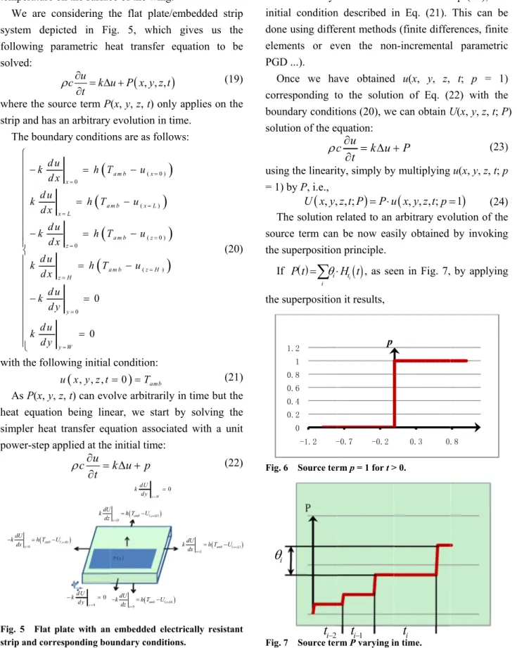
lculations we usually, the the airfoil is ting in the e flight, we e applied and e ) n n ]. l d e e ) e e s e e dat which fr temperature We are c system dep following p solved: where the so strip and has The boun d k d d u k d x d k d d u k d x d k d d u k d y with the foll
As P(x, y, heat equatio simpler heat power-step a
Fig. 5 Flat strip and corr
0 amb x dU k h T dx requency, in on the surfac considering t picted in Fi parametric h u c k t ource term P s an arbitrary dary conditio
0 0 0 0 0 x a x L z a z H y y W u h T d x h T u h T d x h T u d y lowing initial
, , , u x y z t , z, t) can evo on being line t transfer equ applied at the u c t
plate with an responding bou 0 0 y dU k dy x0 U dU k dz order to ob ce of the wing the flat plate ig. 5, which heat transfer
, , , u P x y z P(x, y, z, t) on evolution in ons are as foll
( 0 ) ( ) ( 0 ) ( ) a m b x m b x L a m b z a m b z H T u u T u u l condition:
0 Tamb olve arbitraril ear, we start uation associ e initial time: k u p embedded el undary condit y W dU k dy 0 amb z z dU k h T U dz amb z H z H U h T U btain the des g. e/embedded h gives us equation to
t nly applies on time. lows:
ly in time but t by solving iated with a ectrically resis tions. 0 amb x L dU k h T dx 0 z sired strip the o be (19) n the (20) (21) t the g the unit (22) stant whe sam init don elem PGD O corr bou solu usin = 1) T sou the I the Fig. Fig. x L U i
ere p = 1 in t me boundary ial condition ne using diffe ments or ev D ...). Once we ha responding t undary condit ution of the e c
ng the lineari ) by P, i.e.,
, , U x y The solution r urce term can superposition f i i P t
superposition . 6 Source ter . 7 Source ter 0 0.2 0.4 0.6 0.8 1 1.2 -1.2 -i
2 it
the strip (as s conditions d n described i erent methods ven the non ave obtained to the solutio tions (20), we quation: u c k u t ty, simply by
, , ;z t P P u related to an n be now eas n principle.
i t H t , as se n it results, rm p = 1 for t > rm P varying i -0.7 -0.2 p 1 it
shown in Fig described in E in Eq. (21). s (finite diffe n-incremental d u(x, y, z, on of Eq. (2 e can obtain U P y multiplying
, , , ; u x y z t p arbitrary evo sily obtained en in Fig. 7, > 0. in time. 0.3 0 it
. 6), with the Eq. (20), and This can be rences, finite l parametric t; p = 1) 22) with the U(x, y, z, t; P (23) u(x, y, z, t; p
1 (24) olution of the by invoking by applying .8 e d e e c ) e P) ) p ) e g g
( , , , ) , , , - ; 1 i i i i t t U x y z t
u x y z t t p
(25)4. Numerical Results
4.1 Steady Heating 4.1.1 Airfoil’s Temperature in 2DAs explained in section 2.1, we first have to estimate the convection coefficient. This coefficient h is assumed in first approximation independent of the power induced in the strip and the outside temperature. The only parameter that can influence this coefficient is the free-stream velocity v as the conditions are then comparable to a forced convection.
The expected tendency is reflected in the numerical results, as h changes only according to the free-stream velocity.
For v = 20 m/s, we obtain h = 8.2 W/m2 K. For v = 100 m/s, we obtain h = 18.2 W/m2 K.
For a flat plate 15 cm long, 17.9 mm thick, and a strip of the same length and 0.1 mm thick, solving Eqs. (2), (6) and (7) with the boundary conditions described in Eq. (3), gives us the following temperatures (in the following figures, “I” represents the intensity administered in the electrically resistant strip).
Figs. 8-13 show the influence of the conduction coefficient k and the intensity I applied on the strip. Figs. 14-18 compared to the previous figures let us
Fig. 8 Plate’s temperature for v = 20 m/s, h = 8.2 W/m2K, I = 2 A and k = 300 W/mK.
Fig. 9 Boundary layer’s temperature in contact with the plate, for v = 20 m/s, h = 8.2 W/m2K, I = 2 A and k = 300
W/mK.
Fig. 10 Plate’s temperature for v = 20 m/s, h = 8.2 W/m2K, I = 7 A and k = 300 W/mK.
Fig. 11 Plate’s temperature for v = 20 m/s, I = 2A and k = 100 W/mK.
Fig. 12 Boundary layer’s temperature in contact with the plate, for v = 20 m/s, I = 2 A and k = 100 W/mK.
Fig. 13 Plate’s temperature for v = 20m/s, I = 7A and k = 100 W/mK.
Fig. 14 Plate’s temperature for v = 100m/s, h = 18.2 W/m2K, I = 2 A and k = 300 W/mK.
Fig. 15 Boundary layer’s temperature in contact with the plate, for v = 100 m/s, h = 18.2 W/m2K, I = 2 A and k = 300
W/mK.
Fig. 16 Plate’s temperature for v = 100m/s, h = 18.2 W/m2K, I = 7 A and k = 300 W/mK.
Fig. 17 Plate’s temperature for v = 100 m/s, I = 2 A and
Fig. 18 Boundary layer’s temperature in contact with the plate, for v = 100 m/s, I = 2 A and k = 100 W/mK.
appreciate the influence of the free stream velocity. 4.1.2 3D Plate Temperature—PGD Solution
In this example, we are going to solve the 3D heat transfer equation for a flat plate, i.e., Eq. (10) with the boundary conditions described in Eq. (11) for 7 coordinates: x, y, z (space coordinates), the width of the strip W, the distance between two strips D, the length L and the power in the strip P. Thus, the solution is found under the form:
1 ( ) ( ) i N i i i i i i i i U X x Y y Z z W W D D F L P P
(26)The convection coefficient h and the conduction coefficient k are considered known. The results are shown for two values of each of these parameters: h = 8.2 W/m2·K and h = 18.2 W/m2·K; k = 300 W/mK and
k = 100 W/mK.
The calculation time in order to obtain the solution for all values of the extra-coordinates is approximately 142s. This abacus contains the temperature of all the points on the plate and strip, for all length of the airfoil, width of the strips, distance between two strips and for any power applied. The meshing chosen was 100 values for x, 200 for y, 500 for z, 100 for P, 50 for L, and 20 for W and D, that means 20 × 1013 dof with a traditional
meshing technique, or having to solve 2 × 10⁶ 3D
problems in order to obtain the same information as Eq.
Fig. 19 Plate’s surface temperature for h = 8.2 W/m2K, k
= 300 W/mK, W = 0.289 m, d = 0.289 m, P = 5 × 10⁶ W/m3.
Fig. 20 Plate’s surface temperature for h = 8.2 W/m2K, k
= 300 W/mK, W = 0.1 m, d = 0.48 m, P = 5 × 10⁶ W/m3.
Fig. 21 Plate’s surface temperature for h = 8.2 W/m2K, k
Fig. 22 Plate’s surface temperature for h = 8.2 W/m2K, k
= 100 W/mK, W = 0.289 m, d = 0.289 m, P = 5 × 10⁶ W/m3.
Fig. 23 Plate’s surface temperature for h = 18.2 W/m2K, k
= 300 W/mK, W = 0.289 m, d = 0.289 m, P = 5.106 W/m3.
Fig. 24 Plate’s surface temperature for h = 18.2 W/m2K, k
= 100 W/mK, W = 0.289 m, d = 0.289 m, P = 5 × 10⁶ W/m3.
(26) contains. The parametric solution particularization only takes 0.3 s.
From now on, in order to enable comparison, we only show the plate’s surface temperature in Figs. 19-24. But the temperature of any part of the plate could be shown if wanted.
We can clearly notice in Figs. 19-24 the influence of the convection coefficient (which changes according to the free-stream velocity), the conduction coefficient, the applied power on the strip and the width of these strips.
4.2 Unsteady Heating
In the presented example, we consider a flat plate with the following dimensions:
0 ; 15 ,
0 ; 20 , z
0 ; 0.18
x y
The outside temperature is considered to be Tamb =
20 °C.
The heating strip is located at
3 ; 12 ,
4 ; 8 , z
0.16 ; 0.18
x y .
We first calculate the solution of c u k u p
t
where p = 1 as previously described.
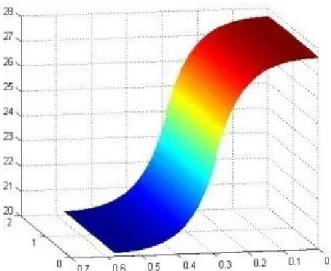
Fig. 25 represents the temperature on the surface of the plate for P = 1. To obtain the solution for P = 2, as shown in Fig. 26, we make use of the linearity.
The temperature on the surface of the plate can easily be seen for one step, two or more, by using superposition.
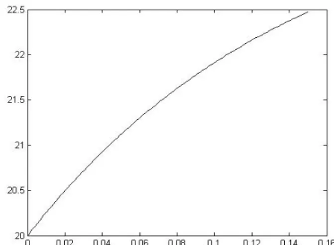
Fig. 27 shows the temperature evolution at the surface of the strip (z = 0.18 cm), where x = 7.5 cm and y = 6 cm with one power step at t1 = 1 and 1 = 6.
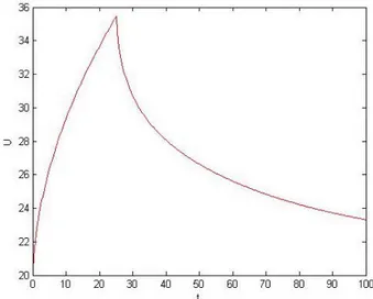
Fig. 28 shows the temperature of the same point and same thermal step than in Fig. 27, but with a second step applied at t2 = 4 with 2 = -6. We can clearly see the
temperature of the plate decreasing as a result of this second impulse. In Figs. 29-30, we can see the temperature at the same point under the influence of a pulsed wave, as we apply P and -P alternatively at every time step. In Fig. 29, the pulse frequency is Dt = 3, and P = 6. In Fig 30, P is doubled, and Dt is divided by 2.
Fig. 25 Temperature on the surface of the plate, at time t = 50, for P = 1.
Fig. 26 Temperature on the surface of the plate, at time t = 50, for P = 2.
Fig. 27 One impulse at time t1 = 0 and 1 = 6.
Fig. 28 Two Impulses at t1 = 0 where 1 = 6, and at t1 = 25
where 1 = -6.
Fig. 29 Impulse at t1 = 0 and 1 = 6 and at t2 = 25 and 2 =
-6 . Thereafter pulse wave every Dt = 3.
Fig. 30 Impulse at t1 = 0 and 1 = 12 and at t2 = 25 and 2 =
5. Conclusions
A new approach to improve fuel consumption during an airplane flight consists in heating the wings. This requires the creation of a numerical abacus in order to know which thermal power must be given to obtain the required temperature as a function of the flight conditions.
In this work, we have seen that it is possible to obtain a simple mathematical model corresponding to the physics: indeed, the 2D models enabled us to define the convection coefficient h, and determine that it is not compulsory to take the boundary layer’s temperature into account to obtain an accurate temperature of the surface of the plate. Instead, it suffices to consider the ambient temperature.
The 3D parametric model helps the design of the airfoil and strip by enabling the evaluation of all design configurations thanks to a faster calculation time. And finally, the 3D unsteady heating model (parametric or not) allows fast unsteady calculus for any given signal.
The ongoing work concerns
We must still define the optimum and control criteria: As the final aim is to improve fuel consumption during a flight, we must determine which would be the compromise between the energy consumption and temperature, both depending on the intensity, length and power step frequency;
A control system based on the numerical PGD abacus (containing all the different parameters) ensuring the right temperature on the surface of the strip, i.e., the inverse identification, must still be defined.
References
[1] F. Masson, F. Chinesta, A. Leygue, E. Cueto, L. Dala, C. Law, Real-time control of the heating of an airfoil, Journal of Materials Science and Engineering A 2 (5) (2012) 478-487.
[2] Dr.H. Schlichting, Boundary-Layer Theory, McGraw-Hill, 1968.
[3] J.D. Anderson, Fundamentals of Aerodynamics,
McGraw-Hill, 1985.
[4] F. Chinesta, P. Ladeveze, E. Cueto, A short review in model order reduction based on Proper Generalized Decomposition, Archives of Computational Methods in Engineering 18 (2011) 395-404.
[5] F. Chinesta, A. Ammar, E. Cueto, Recent advances in the use of the Proper Generalized Decomposition for solving multidimensional models, Archives of Computational Methods in Engineering—State of the Art Reviews 17 (4) (2010) 327-350.
[6] Ch. Ghnatios, F. Chinesta, E. Cueto, A. Leygue, P. Breitkopf, P. Villon, Methodological approach to efficient modelling and optimization of thermal processes taking place in a die: Application to pultrusion, Composites Part A: Applied Science and Manufacturing 42 (2011) 1169-1178.
[7] Ch. Ghnatios, F. Masson, A. Huerta, E. Cueto, A. Leygue, F. Chinesta, Proper Generalized Decomposition based dynamic data-driven control of thermal processes, Computer Methods in Applied Mechanics and Engineering 213-216 (2012) 29-41.
[8] D. Gonzalez, F. Masson, F. Poulhaon, A. Leygue, E. Cueto, F. Chinesta, Proper Generalized Decomposition based dynamic data-driven inverse identification, Mathematics and Computers in Simulation 82 (2012) 1677-1695.
[9] H.J. Bungartz, M. Griebel, Sparse grids, Acta Numerica 13 (2004) 1-123.
[10] E. Cancès, M. Defranceschi, W. Kutzelnigg, C. Le Bris, Y. Maday, Computational quantum chemistry: A primer, Handbook of Numerical Analysis X (2003) 3-270.
[11] P. Ladeveze, Nonlinear Computational Structural Mechanics, Springer, NY, 1999.
[12] P. Ladeveze, J.-C. Passieux, D. Neron, The LATIN multiscale computational method and the Proper Generalized Decomposition, Computer Methods in Applied Mechanics and Engineering 199 (21-22) (2010) 1287-1296.
[13] A. Ammar, B. Mokdad, F. Chinesta, R. Keunings, A new family of solvers for some classes of multidimensional partial differential equations encountered in kinetic theory modelling of complex fluids, J. Non-Newtonian Fluid Mech. (2006).
[14] A. Ammar, B. Mokdad, F. Chinesta, R. Keunings, A new family of solvers for some classes of multidimensional partial differential equations encountered in kinetic theory modelling of complex fluids: Part II. Transient simulation using space-time separated representations, J. Non-Newtonian Fluid Mech. 144 (2007) 98-121.
[15] E. Pruliere, F. Chinesta, A. Ammar, On the deterministic solution of multidimensional parametric models by using the proper generalized decomposition, Mathematics and Computer Simulation 81 (2010) 791-810.