HAL Id: hal-02477077
https://hal.archives-ouvertes.fr/hal-02477077
Submitted on 13 Feb 2020
HAL is a multi-disciplinary open access archive for the deposit and dissemination of sci-entific research documents, whether they are pub-lished or not. The documents may come from teaching and research institutions in France or abroad, or from public or private research centers.
L’archive ouverte pluridisciplinaire HAL, est destinée au dépôt et à la diffusion de documents scientifiques de niveau recherche, publiés ou non, émanant des établissements d’enseignement et de recherche français ou étrangers, des laboratoires publics ou privés.
A Dynamic Bayesian Network Framework for Spatial
Deterioration Modelling and Reliability Updating of
Timber Structures Subjected to Decay
Thanh Binh Tran, Emilio Bastidas-Arteaga, Younes Aoues
To cite this version:
Thanh Binh Tran, Emilio Bastidas-Arteaga, Younes Aoues. A Dynamic Bayesian Network Framework for Spatial Deterioration Modelling and Reliability Updating of Timber Structures Subjected to Decay. Engineering Structures, Elsevier, 2020, �10.1016/j.engstruct.2020.110301�. �hal-02477077�
Please cite this paper as:
Tran, T.-B., Bastidas-Arteaga, E., & Aoues, Y. (2020). A Dynamic Bayesian Network framework for spatial deterioration modelling and reliability updating of timber structures subjected to decay. Engineering
Structures, 209, 110301. https://doi.org/10.1016/j.engstruct.2020.110301
A Dynamic Bayesian Network Framework for Spatial Deterioration
Modelling and Reliability Updating of Timber Structures Subjected to
Decay
Thanh-Binh Tran1, Emilio Bastidas-Arteaga1*, and Younes Aoues2
1 University of Nantes, Institute for Research in Civil and Mechanical Engineering, CNRS UMR 6183, Nantes,
France.
2 Normandie Univ, INSA Rouen Normandie, Laboratoire de Mécanique de Normandie, EA 3828, Rouen,
France.
Abstract
Reliability assessment of existing timber structures subjected to deterioration processes is an important task to evaluate their serviceability and safety levels. Towards this aim, data collected after inspection campaigns are often used for updating structural reliability and planning future maintenance/inspection activities. Under natural conditions, timber decay involves a large number of uncertainties related to material properties and environmental exposure. These uncertainties are also affected by temporal and spatial variability of associated deterioration processes. In this context, the main objective of this study is to propose a Dynamic Bayesian Network approach for updating the structural reliability of deteriorating timber structures using inspection data. The proposed approach can account for the uncertainties in the decay process and the effect of spatial variability. It is also useful for reliability updating considering the uncertainties of inspection techniques. The proposed methodology is illustrated with the reliability updating of a timber beam subjected to decay deterioration. Results indicate that this approach is useful for evaluating and updating of structural reliability from spatially distributed inspection data. Reliability updating could also be carried out from partial observations at given areas, which is very useful for large-scale infrastructure.
Keywords: Spatial Variability; Reliability; Updating; Maintenance; Inspection; Dynamic Bayesian Networks; Timber Decay
List of acronyms
BN: Bayesian Network
COV: Coefficient of Variation
CSRVs: Common Source Random Variables CPTs: Conditional Probability Tables DBN: Dynamic Bayesian Network
DS: Dunnet-Sobel
LN: Log-Normal
NDT: Non Destructive Testing PFA: Probability of False Alarm PoD: Probability of Detection SPE Survival Path Event
1. Introduction
In civil construction, timber is a traditional material that is widely used for various types of structures. For example, there are about 27,000 timber bridges over a total of 40,000 bridges in Australia [1]. By observing historical buildings around the world, it can be seen that timber structures guarantee a long-term service life with high durability level. However, due to its sensitivity to environmental conditions and biological actions, various degradation processes could affect this material – e.g. decay fungi, marine borers, termites etc. Among these phenomena, decay attack is frequently recognised as a main cause leading to unexpected structural failures in timber structures. Decay mechanisms generally reduce the cross section of structural members [2–4]. For example, Kalamees [5] found that a building failed after 10 years because of the damage produced by dry rot (Serpula lacrymans). Serviceability and safety levels of timber deteriorating structures are therefore affected significantly, being far from the design values. For example, Ranjith & Setunge [1] found that for some timber structures over 50 years old, the risk of structural failure is very important. Consequently, reliability assessment of the existing timber structures is necessary to evaluate its serviceability and safety levels.
Reliability assessment is often performed after maintenance campaigns in which inspections are carried out to collect actual information about the structural performance. In this stage, a realistic modelling of the deterioration processes is important to provide rational lifetime assessments. Leicester et al. [2,6] proposed decay deterioration models for exposed timber and timber in-ground contact in Australia. Statistical data for model parameters in decay deterioration were collected in several climate zones and correspond to various timber qualities. These models have been adapted or simplified for others regions. For example, Freitas et al. [7] describe the decay process in Brazil by determining a climate index from regressions. These models could be used for reliability assessment of existing structures; however, this task is difficult because of the high variability of the material properties and their interaction with the decay processes under real environmental conditions.
Performing inspection and maintenance of timber structures are then necessary to provide information about existing structures under real exposure conditions [8]. Data collected after inspection campaigns could be integrated in reliability assessment to re-evaluate the performance and safety of structures. Based on these analyses, appropriate maintenance decisions (repair, replace or do nothing) could be afterwards provided. To account for uncertainty of deterioration processes, reliability assessment of timber structures should be performed in a probabilistic framework. Lourenço et al. [3,9,10] assessed the structural safety of timber structures by using Monte Carlo methods for probabilistic modelling. Ranjith & Setunge [1] used Markov models combined with inspection data for deterioration prediction of timber bridges. Sousa et al. [11] used a Bayesian approach for updating reliability assessment with NDT data. However, these studies did not account for some aspects that might lead to inaccurate assessments such as: the spatial-variability and uncertainties of material properties,
the changes in biological activity or environmental conditions and the imperfection of inspection techniques.
A Bayesian based approach is a suitable tool that could incorporate all these issues for reliability assessment. In the form of multi-events, it turns in the form of Bayesian network (BN) for describing the relationship between random variables. This approach has been used for reliability updating in some previous studies related to timber, concrete or steel durability [12–16]. Dynamic Bayesian Networks (DBN) are extensions of BN to deal with interactions between the components of a system or time-dependencies [17–19]. DBN will be therefore useful to represent the kinetics of deterioration processes such a timber decay. Within this context, this study proposes a framework for reliability assessment that can be updated from inspection data. The proposed framework is able to deal with:
• The time-dependency of structural performance by using DBN;
• The spatial variability of model parameters, deterioration processes or loading modelled as random fields; and
• The quality of inspection techniques that is introduced in terms of Probability of Detection (PoD) and Probability of False Alarm (PFA).
This study focuses on timber decay; however, the proposed framework could be also applied for reliability assessment and updating of steel/concrete structures subjected to other deterioration processes. The methodology could also be used for reliability updating with partial observations, which is very useful for the inspection/monitoring of large structures (bridges, pipelines, etc.) where only some areas of the structural components could be inspected/monitored for practical or economic reasons.
An introduction about BN random fields modelling is provided in section 2. Section 3 presents the decay deterioration model and the construction of DBN for computing structural reliability. Since the proposed approach based on DBN is time-consuming, Section 4 performs a sensitivity analysis to study the influence of some considered approximations for modelling spatial variability. The effect of spatial discretisation is also explored in Section 4. Finally, the whole methodology is illustrated in section 5 with a numerical example where partial simulated inspection data is employed to update structural reliability.
2. Bayesian Network modelling of random fields
Stationary random fields 𝐘(𝑥, 𝜃) are used to model the spatial variability of material properties or model parameters. Stationarity could be reasonably assumed to represent the spatial variability of a deterioration process for a horizontally positioned beam or wall – e.g., for a reinforced concrete beam [20–22]. They are characterised by three parameters: mean (𝜇(),
standard deviation (𝜎() and auto-correlation function (𝜌((). The auto-correlation function describes the correlation between neighbour points belonging to a same structural component. Figure 1 presents a realisation of a one-dimensional random field 𝐘(𝑥, 𝜃), which can be assumed as a representation of one material property, e.g., Young modulus. Due to the spatial correlation, a measurement from one location could provide certain indirect information of other neighbour location if the correlation at these two locations is high. Hence, the measurements at these locations cannot be appropriately represented as independent random variables and random fields can be seen as a better alternative to account for this spatial variability [20,23–25].
Figure 1: Examples of random field and autocorrelation function
By normalising 𝐘(𝑥, 𝜃), we turn into a stationary Gaussian random field 𝐙(𝑥, 𝜃) with zero mean, unit variance and an auto-correlation function 𝜌,, = 𝜌((:
𝐙(𝑥, 𝜃) =𝐘(𝑥, 𝜃) − 𝜇(
𝜎( (1)
Assuming that a vector of random variables 𝐙 = [𝑍1, 𝑍2… , 𝑍4]6is estimated from a random
field 𝐙(𝑥, 𝜃), 𝐙 will be a Gaussian vector with zero mean, unit variance and correlation matrix 𝑅 = 8𝜌9:; = 𝜌((<𝑥9, 𝑥:=, where 𝑛 represents the number of elements in the discretisation of the component length (Figure 1). The vector 𝐙 can be decomposed as a product of a 𝑛 × 𝑛 transformation matrix 𝐓 and a 𝑛 × 1 vector 𝐔 of independent random variables:
𝐙 = 𝐓𝐔 = C t11 ⋯ t1F ⋮ ⋱ ⋮ tF1 ⋯ tFFI J U1 ⋮ UFL (2)
Figure 2 describes a BN representation of Eq. (2) in which correlated random variables 𝑍9, 𝑖 = 1, … , 𝑛 are child nodes that depend on independent random variables 𝑈9, 𝑖 = 1, … , 𝑛 (parent nodes). The correlations among variables are modelled by links between nodes in the BN. The Conditional Probability Tables (CPTs) assigned to each child node 𝑍9 must contain all mutually exclusive states of its parent nodes 𝑈9, 𝑖 = 1, … , 𝑛. Consequently, the size of the CPTs for this BN will be extremely large as 𝑛 increases.
Figure 2: BN modelling of a vector 𝐙 drawn from a random field
Y(x, θ) x (m) Autocorrelation ρΥΥ x (m) Z1 Z2 Z3 . . . Zn U1 U2 U3 . . . Un
To reduce the size of the CPTs, Bensi et al. [17] proposed some methods to eliminate some nodes or some links in the BN or to use Common Source Random Variables (CSRVs). The approach using CSRVs was initially developed by Song and Kang [26] and will be used in this research for modelling the correlation among spatial correlated random variables. The idea of this approach is to describe the correlation among random variables through common parent variables by a special correlation matrix of Dunnet-Sobel (DS) class [27]. The correlation coefficient between 𝑍9 and 𝑍: is presented as 𝜌9: = ∑R <𝑠9Q𝑠:Q=
QS1 , where 𝑚 is the number of
CSRVs and 𝑞 is the 𝑞VW CSRV. The correlated random variables 𝑍
9 therefore can be expressed
as: 𝑍9 = 𝑉9Y1 − Z 𝑠9Q2 R QS1 + Z 𝑠9Q𝑈Q R QS1 (3)
where 𝐔 and 𝐕 are vectors containing independent standard normal random variables. The correlation coefficients 𝑠9Q can be determined by fitting the actual correlation 𝜌9: with a DS class by solving the following nonlinear constrained optimisation problem:
Minimise: ∑ ∑ 8𝜌9: − ∑R <𝑠9Q𝑠:Q= QS1 ; 2 4 :S9]1 4^1 9S1 Subject to: ∑R 𝑟9Q2 ≤ 1, 𝑖 = 1, … , 𝑛 QS1 (4) The BN corresponding to Eq. (3) is shown in Figure 3 in which correlated random variables 𝐙 can be modelled through independent standard random variables 𝐔 and 𝐕.
Figure 3: BN modelling of random field using CSRV
3. Decay deterioration modelling and structural reliability updating
3.1 Decay deterioration in timber structures
Decay deterioration appears when timber structures are subjected to an ideal environment (high moisture and mild temperature) for the development of fungi. Decay in timber occurs after an initial incubation period <𝑡bcd=, and the speed of decay propagation is measured through the
1 Z2 Z3 . . . Zn U1 U2 . . . Um V1 V2 V3 . . . Vn Z 1 Z Z2 Z3 . . . . . . Zi . . . . . . Zn-1 Zn L CSRV Correlated RV Uncorrelated RV
decay rate (𝑟) measured by decay depth per unit of time (mm/year) (Figure 4). Wang et al. [6] proposed a simplified model of decay deterioration (Eq. (5)) in which decay rate is modelled as a function of two parameters taking into account for the climate zone (𝑘fb9RcVg) and the class of wood (𝑘hiij). This model has been developed and verified from a comprehensive experimental database in Australia. The database includes decay processes in 5 Australian places and considers different timber species during 35 years [6][28]. This model will be used to illustrate the proposed methodology; however, other models could also be employed if they are more accurate/representative of the studied deterioration problem.
𝑟 = 𝑘fb9RcVg𝑘hiij (5)
Based on actual statistical data, Leicester et al. [28] proposed values for 𝑘fb9RcVg and 𝑘hiij for
four hazard zones and four durability classes (Table 1 and Table 2). Wang et al. [6] also suggested the coefficient of variations (COV) for 𝑘fb9RcVg and 𝑘hiij by fitting experimental
data obtained from different sites in Australia for timber poles. These random variables are assumed to follow lognormal distributions. Due to the lack of information about the variance of 𝑘fb9RcVg and 𝑘hiij, these values are used for probabilistic analysis in this study.
Figure 4: Decay process over time (adapted from [6]) Table 1: Mean values and COV of 𝑘hiij
Durability class 𝔼[𝑘hiij] COV[𝑘hiij]
1 0.5 0.45
2 0.65 0.55
3 1.15 0.75
4 2.2 0.9
Table 2: Mean values and COV of 𝑘fb9RcVg
Zone 𝔼[𝑘fb9RcVg] COV[𝑘fb9RcVg] A 0.4 0.55 B 0.5 0.55 C 0.65 0.55 D 0.75 0.55 Time, t Rate, r Decay de pt h, d( t) tlag
Assuming that 𝑘hiij and 𝑘fb9RcVg are independent, the variance of the decay rate (r) is: 𝕍[𝑟] = 𝕍[𝑘fb9RcVg]𝕍[𝑘hiij] + 𝕍[𝑘fb9RcVg](𝔼[𝑘hiij])2
+ 𝕍[𝑟𝑘hiij](𝔼[𝑘fb9RcVg])2 (6)
The time to start decay <𝑡bcd= can be described as a function of decay rate 𝑟 as follows:
𝑡bcd = 8.5𝑟^s.tu (7)
Decay depth at given time 𝑡 is calculated as follows: 𝑑(𝑡) = w 0 𝑡 ≤ 𝑡bcd
𝑟<𝑡 − 𝑡bcd= 𝑡 > 𝑡bcd (8) Under decay attack, the cross sections of timber structures are reduced and this reduction significantly influences its reliability and safety. Therefore, during structural lifetime, it is necessary to perform inspections to obtain information about the structural condition. After inspections, several decisions (do nothing, repair or replace) could be undertaken to extend the service life of structures or to ensure reliability thresholds. To provide a practical inspection and repair criterion, Leicester et al. [29] proposed an acceptable depth of surface decay for replacement 𝑑{ ≥ 10 mm. This criterion is used further in this study to define a serviceability limit state function for the timber component in reliability assessment.
3.2 Dynamic Bayesian Networks for reliability assessment of timber beams subjected to decay
Let’s consider a timber beam subjected to decay deterioration. The decay rate (𝑟) is supposed to vary in space and will be modelled as a random field along the beam. For reliability assessment, this beam is divided into 𝑛 elements (Figure 5). Within an element, the deterioration state at time 𝑡 is described through a set of time-variant variables and considered to be uniform.
The limit state function of the 𝑖th element at time 𝑡 (𝑔9,V) defines the event when the decay
depth of 𝑖th element at time 𝑡 (𝑑9,V) reaches the threshold value for replacement 𝑑{ ≥ 10 mm [29]:
𝑔9,V = 𝑑9,V− 10𝑚𝑚 (9)
More complex limit state functions could be also integrated in the proposed framework to account for the mechanical behaviour of a timber beam when considering decay, inspection and spatial variability. This would require considering the uncertainty and spatial variability of other parameters (mechanic, loading, geometry, etc.). However, due to the lack of data to characterise the spatial variability, we prefer to focus on this simple limit state to avoid making additional assumptions about the stationarity and correlation length of these additional parameters.
Figure 5: Discretisation of the timber beam for reliability assessment
Assuming that the timber beam consists of 𝑛 elements is a series system. Hence, the limit state function of this system at time 𝑡 is defined as:
𝑔~•~,V = 𝑔1,V ∪ 𝑔2V∪ … 𝑔9,V ∪ … 𝑔4,V (10)
From Eq. (3) to (10), it is possible to construct a DBN for modelling the performance of the timber structure as shown in Figure (6). This DBN consists of 𝑡 = 1, 2, … , 𝑇 time slices in which 𝑇 can be presented as the service life of structure. In each slice, nodes 𝑔~•~,V represent
the limit state of the beam at the year 𝑡. Nodes 𝑔1,V, 𝑔2,V, … , 𝑔4,V denote the evaluation of the
limit state function at the element level with two discrete states: excessive decay for replacement is or not reached (Eq. 9). Therefore, the conditional probability table (CPTs) 𝑃<𝑔~•~,V„𝑔1,V, 𝑔2,V, … , 𝑔4,V= which is defined from Eq. (10) will have 24]1 entries. When the
number of discretised elements is larger, the size of the CPTs increases also exponentially making the computational and memory demand become infeasible. Bensi et al. [18] proposed efficient BN system models in which performance of a series system could be described by a chain of survival path events (SPE) 𝑆𝑃𝐸9,V, 𝑖 = 1,2, … , 𝑛; 𝑡 = 1, 2, … , 𝑇 which are defined as
follows:
𝑆𝑃𝐸9,V = ‡1 if Š𝑆𝑃𝐸9^1,V = 1‹ ∩ Š𝑔9,V = 1‹
0 otherwise (11)
where 𝑆𝑃𝐸9,V = 1 and 𝑔9,V = 1 denote the survival states and 𝑆𝑃𝐸9,V = 0 denotes failure. At the
first element (𝑖 = 1), the state 𝑆𝑃𝐸1,V is equal to 𝑔1,V, and with 𝑖 > 1, 𝑆𝑃𝐸9,V is survival <𝑆𝑃𝐸9,V = 1= only if both 𝑆𝑃𝐸9^1,V and 𝑔9,V are survival <𝑆𝑃𝐸9^1,V = 1 𝑎𝑛𝑑 𝑔9,V = 1=. The state of the system <𝑔~•~,V= is equal to the state of the last element <𝑆𝑃𝐸4,V= and hence, the CPT of
node 𝑔~•~,V is defined with only four entries and the computational demand is reduced
significantly [18].
Nodes 𝑑1,V, 𝑑2,V, … , 𝑑4,V and 𝑟1,V, 𝑟2,V, … , 𝑟4,V respectively denote decay depth and decay rate at
𝑖th element. The conditional probability 𝑃<𝑔9,V„𝑑9,V=, with 𝑡 = 0 or 𝑃<𝑔9,V„𝑑9,V, 𝑔9,V^1=, with
𝑡 > 0 and 𝑃<𝑑9,V„𝑟9,V=, with 𝑡 = 0 or 𝑃<𝑑9,V„𝑟9,V, 𝑑9,V^1=, with 𝑡 > 0 are calculated based on Eq. (9) and (8), respectively. The spatial correlation of the decay rate (𝑟) among elements is described by Eq. (3) through 𝑚 Common Source Random Variables and 𝑛 independent standard random variables. The probability 𝑃<𝑟9,V„𝑟9,V^1= is a unit matrix since 𝑟9,V is
time-invariant.
The observation 𝑂9,V is defined as the value of inspection at 𝑖th element and time 𝑡. Due to the lack of a real study case, we will consider in sections 4.3 and 5 various inspection outcomes
1 Z2 Z3 . . . Zn U1 U2 . . . Um V1 V2 V3 . . . Vn Z 1 Z Z2 Z3 . . . . . . Zi . . . . . . Zn-1 Zn L CSRV Correlated RV Uncorrelated RV
with different levels of uncertainty. It is supposed that the outcome of an inspection is to detect if the decay depth is larger than the critical value for replacement 𝑑{ ≥ 10 mm [29] for the 𝑖th
element. These observations could be obtained by using different inspection techniques to assess the decay depth in timber structures, e.g. ultrasound resistance drilling or pin penetration tests [11]. Results from these inspections give information whether 𝑖th component is failing (detection) or not failing (no detection) with respect to the limit state function Eq. (9). The uncertainty of inspections will depend on the selected technique and is represented by the conditional probabilities 𝑃<𝑂9,V„𝑔9,V=. Depending on the outcome of the inspection (detection or not detection) and the action after inspection (replacement or not replacement), two probabilities could be defined: Probability of Detection (PoD) and Probability False Alarm (PFA) (Table 3). A detailed definition of PoD and PFA is found in [30]. Specific tests could be conducted to estimate PoD and PFA for a given inspection technique. Since this work is not focusing on a given technique, the effect of several levels of PoD and PFA will be studied and discussed in section 4.3.
Table 3: PoD and PFA represent for quality of decay assessment method 𝑂9,V= Detection 𝑂9,V = No detection
𝑔9,V= replacement PoD 1 – PoD
𝑔9,V = no replacement PFA 1 – PFA
Figure 6: DBN modelling decay deterioration of timber structures
4. Sensitivity analysis when considering the spatial variability
Considering the spatial variability of model parameters is important to obtain a more realistic reliability assessment. However, to include this behaviour in DBN modelling of structure’s performance is a difficult task due to the large number of correlated random variables resulting from the discretisation. This will lead to a densely connected BN where the computation demand becomes intractable [17]. A solution for this issue was detailed in Section 2 and lies
1,0 r2,0 r3,0 . . . rn,0 U1 U2 . . . Um V1 r V2 V3 Vn 1,0 d2,0 d3,0 . . . dn,0 d 1,0 g Slice t = 0 2,0 g g3,0 gn,0 1,0 SPE gsys,0 1,T r2,T r3,T rn,T r 1,T d2,T d3,T . . .dn,T d 1,T g g2,T g3,T gn,T 1,T SPE g sys,T Slice t = 1 Slice t = T 2,T
SPE SPE3,T SPEn,T 1,1 r2,1 r3,1 rn,1 r 1,1 d2,1 d3,1 . . .dn,1 d 1,1 g g2,1 g3,1 gn,1 1,1 SPE gsys,1 2,1
SPE SPE3,1 SPEn,1 2,0
SPE SPE3,0 SPEn,0
1,1
O O2,1 O3,1 On,1 O1,T O2,T O3,T On,T
1,0
in approximating the correlation among random variables to simplify the BN. We considered in this analysis the effect of spatial variability of decay by assuming that it could be represented as a random stationary field (section 2). The correlation length is a parameter used to quantify and model the spatial correlation among random variables. This value could be estimated from experimental data and will differ depending on the studied problem [21,22]. Due to the lack of experimental data, it is not possible to test the stationarity assumption and to determine the correlation length. Since the correlation length is the most influencing parameter describing the spatial variability of a stationary random field, a sensitivity analysis is performed to study its effect of reliability assessment in Section 4.1.
The sensitivity analysis presented in this section considers the effects of: (1) the number of elements from structural discretisation and the correlation length, (2) the number of CSRVs and (3) the quality of inspection techniques. The sensitivity analysis will be applied to a timber beam with 𝐿 = 6000mm length subjected to decay deterioration (Figure 5). It is assumed that this beam is built using class 1 timber and it is located in zone A. According to Equations (5) and (6) and Tables (1) and (2), the decay rate follows a lognormal (LN) distribution with the mean value and coefficient of variation presented in Table 4. These values are used in the following studies excepting when a sensitivity analysis is carried out.
In section 4.1 and 4.2 we consider that the inspection is perfect (PoD =1.00 and PFA=0) and in section 4.3, different values of PoD and PFA are introduced to study the influence of the quality of the inspection technique. We only consider in this study discrete variables, therefore each node in DBN should be discretised into finite number of states. Table 5 presents the discretisation of parameters and their boundaries, which are sufficiently large to cover most of their possible values. The number of states and the boundaries were defined to balance accuracy and computational cost.
Table 4: Parameters of the timber beam
Parameter Description Value
𝐿(𝑚𝑚) Length 6000
𝑏(𝑚𝑚) Correlation length 3000
𝑟(𝑚𝑚/𝑦𝑒𝑎𝑟) Decay rate LN(𝔼[𝑟] = 0.2; COV[𝑟] = 0.75)
𝑛 Number of elements 25
𝑛_𝐶𝑆𝑅𝑉 Number of CSRV 4
Table 5: Discretisation of parameters Nodes Number of states Boundaries
𝑟9,V(𝑚𝑚/𝑦𝑒𝑎𝑟) 10 [0; 5]
𝑔9,V Binary –
𝑆𝑃𝐸9,V Binary –
𝑔~•~V Binary –
4.1 Influence of structural discretisation and correlation length on the assessment of structural reliability
To consider the spatial variability of the decay rate, timber structures are divided into 𝑛 elements for reliability analysis. The length of each element should be smaller than the correlation length to account for the spatial correlation between 𝑍9 elements. However, in
practice, it is very difficult to determine accurately the correlation length for specific structures. Different assumptions about correlation length may lead to different outputs in reliability assessment. Based on this context, this section aims at investigating the effect of structural discretisation and correlation length on reliability assessment.
Figure 7 depicts the probability of failure, 𝑃¡, of the beam when spatial variability is considered
by discretising the beam into different number of elements. It can be seen that considering spatial variability has an important influence on the assessment of 𝑃¡. When the beam is divided in a high number of elements, larger values of 𝑃¡ are expected. This trend is also due to the
nature of the limit state function of a series system defined by Eq. (10). For a series system, the failure of one element implies the failure of the system. Thus, with small or no correlation between the elements, 𝑃¡ will be large when the number of elements increases. However, when the correlation among elements is considered, spatial variability affects the reliability analysis of the beam depending on both the correlation length and discretisation. The discretisation should be small enough to account for the spatial variability. Then by increasing the number of elements, it is noted in Figure 7 that there is a convergent trend on the assessment of the failure probability. In this case, the value of 𝑃¡ is convergent when the discretisation of the
beam is made by at least 25 elements. Thus, this discretisation will be used in the following computations.
Figure 7: Probability of failure of the beam with consideration of spatial variability
0 10 20 30 40 Time (year) 0 0.1 0.2 0.3 0.4 0.5 0.6 Probability of Failure 3 elements 5 elements 10 elements 14 elements 18 elements 22 elements 25 elements 27 elements 30 elements
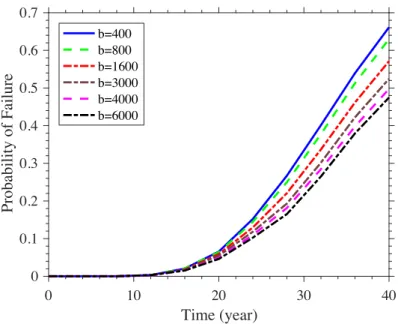
If 𝑛 = 25 elements, Figure 8 presents the assessment of 𝑃¡ with different values of correlation length (𝑏). It is observed that the correlation length has significant influence on the prediction of 𝑃¡. Theoretically, when the correlation length increases, the correlation between two elements is higher and thus, the variability of the considered parameters between two elements becomes less important. This behaviour explains the lower prediction of 𝑃¡ when 𝑏 increases. On the contrary, if the correlation length is small, the correlation among elements is weak leading to higher values of 𝑃¡.
Figure 8: Probability of failure of the beam with different correlation lengths (in mm)
4.2 Effect of the approximation of the correlation coefficient on the assessment of structural reliability
In this study, the correlation among random variables is modelled using CSRVs. A more accurate approximation of the correlation coefficient requires a large number of CSRVs. This section aims at studying the influence of the number of CSRV on reliability assessment. The analysis is based on the comparison the probability of failure of system or elements with different number of CSRVs used to describe the correlation among random variables. In this section it is considered that the timber beam is divided into 𝑛 = 25 elements. Inspection is performed on the first element at the age of 24 years and inspection indicates failure. This inspection date was defined based on the probability of failure of the elements at this age. It could be observed in Figure 13b that the prior probability of failure for the elements varies between 10-3 and 10-2 from the 20 to 28 years, respectively. Based on this range, we considered
that the structure was inspected at 24 years because, at this date, the probability of failure is close to the threshold value for a serviceability limit state defined by the Eurocode for a reference period of 50 years (𝛽=1.5, 𝑃¡ ≈ 6.7×10⁻²). Thus, it is possible to assume that
inspection outcomes could be “fail” or “not fail” at this date.
We also assume that the auto-correlation function of the decay random field follows an exponential function (Eq. (12)) that depends on the correlation length 𝑏. Figure 9 compares the approximate correlation coefficients estimated when different numbers of CSRV are used. It is clear that, to minimise the approximation errors, it is necessary to use more CSRVs. The
0 10 20 30 40 Time (year) 0 0.1 0.2 0.3 0.4 0.5 0.6 0.7 Probability of Failure b=400 b=800 b=1600 b=3000 b=4000 b=6000
approximate autocorrelation values obtained from fitting with 4 CSRVs are close to the correlation coefficients estimated from Eq. (12). Therefore, for further analysis in this paper, we use 4 CSRV for modelling the correlation among random variables.
𝜌<𝑥9, 𝑥:= = 𝑒𝑥𝑝 ¤−„𝑥9 − 𝑥:„
𝑏 ¥ (12)
Figure 9: Comparison between modelled and estimated autocorrelation values
Figure 10 provides the prior and updated probability of element failure with different number of CSRVs. Updated probabilities were estimated by introducing the evidence in the DBN for the inspection of the first element at 24 years that resulted in failure (a decay rate higher than 10mm). The horizontal axis represents the distances of other elements along the beam from the first element. When no inspection is performed, elements at different locations almost have the same probabilities of failure, being in the range [2×10⁻³; 6×10⁻³] at the age 24 years (Figure
10a). A similar range was obtained by using Monte Carlo simulations and Karhunen-Loève expansion [31] to validate the DBN results. Due to the correlation among elements, information from one location along the timber beam could provide certain information for its neighbour elements. This aspect links to practical issues that inspection data from one location could give information about damage state of other locations. We assume that inspection at the first element indicates failure state; hence it is expected to have higher probability of failure of elements located close to the first one as compared to their prior 𝑃¡. This trend is observed in Figure 10b with a decreasing shape in 𝑃¡ when the distance from the first element increases. However, with a high number of CSRVs, the fluctuation of the update probability of failure in Figure 10b could be reduced significantly. For all the cases, when the distance is larger than the correlation length (∆§> 𝑏 = 3000𝑚𝑚), the correlation between elements is weak, hence the updated 𝑃¡ lead to lower values. This trend is observed more clearly in Figure 11 where a sensitivity analysis is performed with different correlation lengths. When the correlation between elements is high (𝑏 is larger), higher values of updated 𝑃¡ are obtained. The values of 𝑃¡ are smaller for elements far from the first element (failing element).
0 1000 2000 3000 4000 5000 6000
Distance to the 1st element(mm) 0 0.2 0.4 0.6 0.8 1 Autocorrelation Original by Eq. (12) 1 CSRV 2 CSRV 3 CSRV 4 CSRV
Figure 10: a) Prior and b) updated probability of failure of elements at different distances from the first element
Figure 11: Updated probability of failure of elements with different values of correlation length
4.3 Effect of quality of inspection techniques
This section examines the effect of the accuracy of the inspection technique that depends on two parameters: PoD and PFA. Supposing that inspection on the first component results in failure, Figure 12a presents the updated 𝑃¡ of other elements. In Figure 12a, if there is no false alarm (PFA=0%), the updated 𝑃¡ indicates that the results for the cases PoD = 70%, 80% and 90% are close to the obtained for a perfect inspection (PoD=100%, PFA=0%). However, Figure 12b reveals that the quality of inspection techniques is very sensitive to the PFA. With PFA > 5%, the updated 𝑃¡ is significantly different to the perfect inspection. When PFA > 20%, the updated 𝑃¡ is very close to its prior value and it seems that there is no influence of spatial variability on the results. Hence, this result highlights the importance to improve the PFA indicator of the inspection technique for having a good reliability assessment.
0 1000 2000 3000 4000 5000 6000
Distance to first element (mm)
0 0.02 0.04 0.06 0.08 Probability of Failure 1 CSRV 2 CSRV 3 CSRV 4 CSRV 0 1000 2000 3000 4000 5000 6000
Distance to first element (mm)
0 0.02 0.04 0.06 0.08 Probability of Failure 1 CSRV 2 CSRV 3 CSRV 4 CSRV (b) (a) 0 1000 2000 3000 4000 5000 6000 Distance to first element (mm) 3 3.5 4 4.5 5 5.5 Probability of Failure 10-3 0 1000 2000 3000 4000 5000 6000
Distance to the first element(mm) 0 0.05 0.1 0.15 Probability of Failure b=400 b=800 b=1600 b=3000 b=4000 b=6000
Figure 12: Sensitivity analysis of inspection accuracy: (a) With PFA=0% and various PoD, and (b) With PoD=100% and various PFA
5. Updating structural reliability with partial inspection data
The updating of structural reliability is an important issue for existing timber structures subjected to deterioration processes. This process requires collecting data about the condition of structures and integrating these data for updating structural reliability. The outputs are useful to plan cost-effective maintenance actions. Nevertheless, for economic or practical reasons (accessibility) it is not always possible to inspect along the beam. Then this section explores how the proposed approach is able to deal with information obtained from partial inspections. For the sake of simplicity, the configuration of the timber beam described in Table 4 is considered in this section. It is assumed that inspections are performed 24 years after the construction of the timber beam to evaluate the damage due to decay attack. Measurements are taken at different elements and afterwards, this data is introduced in the DBN for updating the probability of failure of the beam. It is considered that all measurements at inspected elements indicate the safe state.
Figure 13 depicts the results of the updating of 𝑃¡ when some elements along the beam are inspected. For example, if 5 elements among 25 elements are inspected, they are equidistantly located at the positions: 𝑖 = 1, 7, 13, 19, and 25. It is supposed here that all the inspections were carried out at 24 year and resulted in no detection of excessive decay. It is observed that the updated probabilities are lower than the prior prediction because inspections resulted in no detection of excessive decay. When more elements are inspected, these posterior probabilities are lower (Figure 13a). This trend is expected due to the relationships in a series system (Eq. (10)). In real practice, it is difficult to inspect all elements, especially in the case of large-scale structures. Therefore, this methodology is useful to update the reliability when some parts of structures are inspected. Due to the correlation among elements, information from uninspected elements is also updated. If inspection data indicates a safe state, the updated values for uninspected elements are lower than its prior values (Figure 13b).
0 1000 2000 3000 4000 5000 6000
Distance to first element (mm)
2 4 6 8 10 12 Probability of Failure 10-3 PFA=5 PFA=10 PFA=20 PFA=30 0 1000 2000 3000 4000 5000 6000
Distance to first element (mm)
0 0.02 0.04 0.06 0.08 0.1 0.12 Probability of Failure PoD=70 PoD=80 PoD=90 PoD=100 (a) (b)
Figure 13: Updating of the probability of failure with inspection data at 24 years: (a) beam, and (b) elements
6. Conclusions and perspectives
This paper presented a methodology for modelling and updating reliability of structures subjected to deterioration processes. Dynamic Bayesian Networks were used for modelling decay and updating the reliability assessment with inspection data. The spatial variability of model parameters was introduced in DBN through Common Source Random Variables (CSRVs). CSRVs allow approximating the correlation among elements, and therefore, are useful to reduce the complexity (and computational requirements) of DBNs.
The proposed approach was illustrated with a numerical study case focusing on the assessment of the reliability of a timber beam subjected to decay. A sensitivity analysis was performed to analyse the effects on reliability assessment of: (1) the spatial variability (2) the number of CSRVs used in the approximation and of elements in structural discretisation, and (3) the inspection quality. The results showed that this approach is useful for modelling and updating structural reliability with partial inspection data. Minimum values for the number of CSRVs, the number of elements in the structural discretisation, and PFA are required to ensure consistent reliability assessments. The last part of the paper showed that it is possible to update reliability with partial observations. This finding is useful for reliability assessment of large-scale structures (e.g, the monitoring and inspection of a large bridge), where only information in some parts of the structure is available. However, since spatial correlation requires a significant number of elements to discretise the structure, the computational time could become intractable. More efficient algorithms (e.g., [32]) could be implemented for efficient inference and to decrease the computational time in such a case. This can be seen as one major limitation of this methodology.
Further work will focus on testing the methodology with a real study case. This should include a realistic study case in which spatially distributed data will be used to test and improve the proposed framework. Future works will be also oriented in adapting the proposed methodology to develop a decision-making tool that could be useful to optimise inspection/maintenance operations. Optimised solutions should account for specific environmental conditions and the durability performance of the selected timber. Various repair actions (replacement, reinforcement with fibre-reinforced polymer, etc.) could be also integrated in the formulation of optimal inspection and maintenance strategies.
0 10 20 30 40 Time (year) 0 0.01 0.02 0.03 0.04 Probability of Failure Prior Inspected elements Uninspected elements (b) 0 10 20 30 40 Time (year) 0 0.1 0.2 0.3 0.4 0.5 0.6 Probability of Failure Prior 5 elements 9 elements 13 elements 25 elements (a)
Acknowledgements
The authors would like to acknowledge the financial support of project CLIMBOIS ANR-13-JS09-0003-01 as well as the labelling of the ViaMéca French cluster.
References
[1] S. Ranjith, S. Setunge, Deterioration Prediction of Timber Bridge Elements Using the Markov Chain, J. Perform. Constr. Facil. 27 (2011) 319–325. https://doi.org/10.1061/(ASCE)CF.1943-5509.0000311. [2] R.H. Leicester, C. Wang, M.N. Nguyen, C.E. MacKenzie, Design of Exposed Timber Structures, 9 (2009)
217.
[3] P.B. Lourenço, H.S. Sousa, R.D. Brites, L.C. Neves, In situ measured cross section geometry of old timber structures and its influence on structural safety, Mater. Struct. 46 (2012) 1193–1208. https://doi.org/10.1617/s11527-012-9964-5.
[4] R.K. Lumor, J.S. Ankrah, S. Bawa, E.A. Dadzie, O. Osei, Rehabilitation of timber bridges in Ghana with case studies of the Kaase Modular Timber Bridge, Eng. Fail. Anal. 82 (2017) 514–524.
https://doi.org/10.1016/j.engfailanal.2017.04.003.
[5] T. Kalamees, Failure analysis of 10 year used wooden building, Eng. Fail. Anal. 9 (2002) 635–643. https://doi.org/10.1016/S1350-6307(02)00025-0.
[6] C. Wang, R.H. Leicester, M. Nguyen, Probabilistic procedure for design of untreated timber poles in-ground under attack of decay fungi, Reliab. Eng. Syst. Saf. 93 (2008) 476–481.
https://doi.org/10.1016/j.ress.2006.12.007.
[7] R.R. Freitas, J.C. Molina, C. Calil, Mathematical Model for Timber Decay in Contact with the Ground Adjusted for the State of Sao Paulo, Brazil, Mater. Res.-Ibero-Am. J. Mater. 13 (2010) 151–158. [8] J. Huan, D. Ma, W. Wang, Z. Wang, Safety State Evaluation Method Based on Attribute Recognition
Model for Ancient Timber Buildings, Adv. Civ. Eng. (2019). https://doi.org/10.1155/2019/3612535. [9] R.D. Brites, L.C. Neves, J. Saporiti Machado, P.B. Lourenço, H.S. Sousa, Reliability analysis of a timber
truss system subjected to decay, Eng. Struct. 46 (2013) 184–192. https://doi.org/10.1016/j.engstruct.2012.07.022.
[10] P.C. Ryan, M.G. Stewart, N. Spencer, Y. Li, Reliability assessment of power pole infrastructure incorporating deterioration and network maintenance, Reliab. Eng. Syst. Saf. 132 (2014) 261–273. https://doi.org/10.1016/j.ress.2014.07.019.
[11] H.S. Sousa, J.D. Sorensen, P.H. Kirkegaard, J.M. Branco, P.B. Louren??o, On the use of NDT data for reliability-based assessment of existing timber structures, Eng. Struct. 56 (2013) 298–311.
https://doi.org/10.1016/j.engstruct.2013.05.014.
[12] T.-B. Tran, E. Bastidas-Arteaga, F. Schoefs, Improved Bayesian network configurations for probabilistic identification of degradation mechanisms: application to chloride ingress, Struct. Infrastruct. Eng. In Press (2015) 1–15. https://doi.org/10.1080/15732479.2015.1086387.
[13] T.-B. Tran, E. Bastidas-Arteaga, F. Schoefs, Improved Bayesian network configurations for random variable identification of concrete chlorination models, Mater. Struct. (2016).
https://doi.org/10.1617/s11527-016-0818-4.
[14] Y. Ma, L. Wang, J. Zhang, Y. Xiang, Y. Liu, Bridge Remaining Strength Prediction Integrated with Bayesian Network and In Situ Load Testing, J. Bridge Eng. ASCE. 19 (2014) 1–11.
https://doi.org/10.1061/(ASCE)BE.1943-5592.0000611.
[15] T.-B. Tran, E. Bastidas-Arteaga, Y. Aoues, C.F.P. Nziengui, S.E. Hamdi, R.M. Pitti, E. Fournely, F. Schoefs, A. Chateauneuf, Reliability assessment and updating of notched timber components subjected to environmental and mechanical loading, Eng. Struct. 166 (2018) 107–116.
https://doi.org/10.1016/j.engstruct.2018.03.053.
[16] W. Zheng, Y. Yu, Bayesian Probabilistic Framework for Damage Identification of Steel Truss Bridges under Joint Uncertainties, Adv. Civ. Eng. (2013). https://doi.org/10.1155/2013/307171.
[17] M. Bensi, A. Der Kiureghian, D. Straub, Bayesian network modeling of correlated random variables drawn from a Gaussian random field, Struct. Saf. 33 (2011) 317–332.
https://doi.org/10.1016/j.strusafe.2011.05.001.
[18] M. Bensi, A. Der Kiureghian, D. Straub, Efficient Bayesian network modeling of systems, Reliab. Eng. Syst. Saf. 112 (2013) 200–213. https://doi.org/10.1016/j.ress.2012.11.017.
[19] J. Hu, L. Zhang, W. Tian, S. Zhou, DBN based failure prognosis method considering the response of protective layers for the complex industrial systems, Eng. Fail. Anal. 79 (2017) 504–519.
[20] F. Schoefs, E. Bastidas-Arteaga, T.V. Tran, G. Villain, X. Derobert, Characterization of random fields from NDT measurements: A two stages procedure, Eng. Struct. 111 (2016) 312–322.
https://doi.org/10.1016/j.engstruct.2015.11.041.
[21] N. Rakotovao Ravahatra, F. Duprat, F. Schoefs, T. de Larrard, E. Bastidas-Arteaga, Assessing the Capability of Analytical Carbonation Models to Propagate Uncertainties and Spatial Variability of Reinforced Concrete Structures, Front. Built Environ. 3 (2017). https://doi.org/10.3389/fbuil.2017.00001. [22] N. Rakotovao Ravahatra, E. Bastidas-Arteaga, F. Schoefs, F. Duprat, T. De Larrard, M. Oumouni,
Characterisation and propagation of spatial fields in deterioration models: application to concrete carbonation, Eur. J. Environ. Civ. Eng. In Press (2019). https://doi.org/10.1080/19648189.2019.1620133. [23] A.J. O’Connor, O. Kenshel, Experimental Evaluation of the Scale of Fluctuation for Spatial Variability
Modeling of Chloride-Induced Reinforced Concrete Corrosion, J. Bridge Eng. (2013) 3–14. https://doi.org/10.1061/(ASCE)BE.1943-5592.0000370.
[24] O. Pasqualini, F. Schoefs, M. Chevreuil, M. Cazuguel, Measurements and statistical analysis of fillet weld geometrical parameters for probabilistic modelling of the fatigue capacity, Mar. Struct. 34 (2013) 226– 248. https://doi.org/10.1016/j.marstruc.2013.10.002.
[25] M.G. Stewart, J.A. Mullard, Spatial time-dependent reliability analysis of corrosion damage and the timing of first repair for RC structures, Eng. Struct. 29 (2007) 1457–1464.
https://doi.org/10.1016/j.engstruct.2006.09.004.
[26] J. Song, W.H. Kang, System reliability and sensitivity under statistical dependence by matrix-based system reliability method, Struct. Saf. 31 (2009) 148–156. https://doi.org/10.1016/j.strusafe.2008.06.012. [27] C.W. Dunnet, M. Sobel, Approximations to the probability integral and certain percentage points of a
multivariate analogue of Student’s t-distribution, Biometrika. 42 (1955) 258–260.
[28] R.H. Leicester, C.-H. Wang, M.N. Nguyen, J.D. Thornton, G. Johnson, D. Gardner, G.C. Foliente, C.E. MacKenzie, An engineering model for the decay of timber in-ground contact, in: 34th Int. Conf. Int. Res. Group Wood Preserv. IRG, Brisbance, Australia, 2003.
[29] R.H. Leicester, M. Nguyen, C.-H. Wang, Manual10 – Commentary on a Proposed Timber Service Life Design Code, Australia, 2007.
[30] F. Schoefs, A. Clément, A. Nouy, Assessment of ROC curves for inspection of random fields, Struct. Saf. 31 (2009) 409–419.
[31] R. Ghanem, P. Spanos, Stochastic Finite Elements: A Spectral Approach, Revised edition, Dover Civil and Mechanical Engineering, 2012.
[32] M.T. Bensi, A. Der Kiureghian, D. Straub, A Bayesian Network Methodology for Infrastructure Seismic Risk Assessment and Decision Support, University of California,Berkeley, 2011.


![Figure 4: Decay process over time (adapted from [6]) Table 1: Mean values and COV of](https://thumb-eu.123doks.com/thumbv2/123doknet/11473146.291902/7.892.272.622.495.710/figure-decay-process-time-adapted-table-mean-values.webp)