HAL Id: hal-01852560
https://hal.archives-ouvertes.fr/hal-01852560v2
Submitted on 7 Mar 2019
HAL is a multi-disciplinary open access
archive for the deposit and dissemination of
sci-entific research documents, whether they are
pub-lished or not. The documents may come from
teaching and research institutions in France or
abroad, or from public or private research centers.
L’archive ouverte pluridisciplinaire HAL, est
destinée au dépôt et à la diffusion de documents
scientifiques de niveau recherche, publiés ou non,
émanant des établissements d’enseignement et de
recherche français ou étrangers, des laboratoires
publics ou privés.
Copyright
Analysis and calibration of a linear model for structured
cell populations with unidirectional motion : Application
to the morphogenesis of ovarian follicles
Frédérique Clément, Frédérique Robin, Romain Yvinec
To cite this version:
Frédérique Clément, Frédérique Robin, Romain Yvinec. Analysis and calibration of a linear model for
structured cell populations with unidirectional motion : Application to the morphogenesis of ovarian
follicles. SIAM Journal on Applied Mathematics, Society for Industrial and Applied Mathematics,
2019, 79 (1), pp.207-229. �10.1137/17M1161336�. �hal-01852560v2�
ANALYSIS AND CALIBRATION OF A LINEAR MODEL FOR STRUCTURED CELL POPULATIONS WITH UNIDIRECTIONAL
MOTION: APPLICATION TO THE MORPHOGENESIS OF OVARIAN FOLLICLES\ast
FR \'ED \'ERIQUE CL \'EMENT\dagger , FR \'ED \'ERIQUE ROBIN\dagger , AND ROMAIN YVINEC\ddagger
Abstract. We analyze a multitype age-dependent model for cell populations subject to unidirec-tional motion in both a stochastic and deterministic framework. Cells are distributed into successive layers; they may divide and move irreversibly from one layer to the next. We adapt results on the large-time convergence of PDE systems and branching processes to our context, where the Perron--Frobenius or Krein--Rutman theorem cannot be applied. We derive explicit analytical formulas for the asymptotic cell number moments and the stable age distribution. We illustrate these results numerically and apply them to the study of the morphodynamics of ovarian follicles. We prove the structural parameter identifiability of our model in the case of age independent division rates. Using a set of experimental biological data, we estimate the model parameters to fit the changes in the cell numbers in each layer during the early stages of follicle development.
Key words. structured cell populations, multitype age dependent branching processes, renewal equations, McKendrick--Von Foerster model, parameter calibration, structural identifiability
AMS subject classifications. 35L65, 60K15, 60J80, 92D25
DOI. 10.1137/17M1161336
1. Introduction. We study a multitype age-dependent model in both a de-terministic and stochastic framework to represent the dynamics of a population of cells distributed into successive layers. The model is a two dimensional structured model---cells are described by a continuous age variable and a discrete layer index variable. Cells may divide and move irreversibly from one layer to the next. The cell division rate is age and layer dependent, and is assumed to be bounded below and above. After division, the age is reset and the daughter cells either remain within the same layer or move to the next. In its stochastic formulation, our model is a multitype Bellman--Harris branching process, and in its deterministic formulation it is a multitype McKendrick--Von Foerster system.
The model enters the general class of linear models leading to Malthusian ex-ponential growth of the population. In the partial differential equation (PDE) case, state-of-the-art methods turn to a system of renewal equations [6] or to an eigenvalue problem and general relative entropy techniques [7, 9] to show the existence of an at-tractive stable age distribution. Yet, in our case, the unidirectional motion prevents us from applying the Krein--Rutman theorem to solve the eigenvalue problem. As a consequence, we follow a constructive approach and explicitly solve the eigenvalue problem. On the other hand, we adapt entropy methods using weak convergences in L1 to obtain the large-time behavior and lower bound estimates of the speed of
convergence towards the stable age distribution. In the probabilistic case, classical methods rely on renewal equations [2] and martingale convergences [3]. Using the
\ast Received by the editors December 14, 2017; accepted for publication (in revised form) October 22,
2018; published electronically February 5, 2019.
http://www.siam.org/journals/siap/79-1/M116133.html
\dagger Inria, Universit\'e Paris-Saclay, 1 rue Honor\'e d'Estienne d'Orves, 91120 Palaiseau, France; LMS,
Ecole Polytechnique, CNRS, Universit\'e Paris-Saclay, 91120 Palaiseau Cedex, France (frederique. clement@inra.fr, frederique.robin@inra.fr).
\ddagger PRC, INRA, CNRS, IFCE, Universit\'e de Tours, 37380 Nouzilly, France (romain.yvinec@inra.fr).
same eigenvalue problem as in the deterministic study, we derive a martingale conver-gence giving insight into the large-time fluctuations around the stable state. Again, due to the lack of reversibility in our model, we cannot apply the Perron--Frobenius theorem to study the asymptotics of the renewal equations. Nevertheless, we manage to derive explicitly the stationary solution of the renewal equations for the cell number moments in each layer as in [2]. We recover the deterministic stable age distribution as the solution of the renewal equation for the mean age distribution.
The theoretical analysis of our model highlights the role of one particular layer: the leading layer is characterized by a maximal intrinsic growth rate which turns out to be the Malthus parameter of the total population. The notion of a leading layer is a tool to understand qualitatively the asymptotic cell dynamics, which appears to operate in a multi-scale regime. All the layers upstream from the leading one may become extinct or grow with a rate strictly inferior to the Malthus parameter. The remaining downstream layers are driven by the leading layer: they grow exactly at the same rate as the Malthus parameter, which overcomes their intrinsic growth rates.
We then check and illustrate numerically our theoretical results. In the stochastic case, we use a standard implementation of an exact stochastic simulation algorithm. In the deterministic case, we design and implement a dedicated finite volume scheme adapted to the nonconservative form that deals with proper boundary conditions. We verify that both the deterministic and stochastic simulated distributions agree with the analytical stable age distribution. Moreover, the availability of analytical formulas helps us to study the influence of the parameters on the asymptotic proportion of cells, Malthus parameter, and stable age distribution.
Finally, we consider the specific application of ovarian follicle development in-spired by the model introduced in [1] that represents the proliferation of somatic cells and their organization in concentric layers around the germ cell. While the original model is formulated with a nonlinear individual-based stochastic formalism, we design a linear version based on branching processes and endowed with a straightforward de-terministic counterpart. We prove the structural parameter identifiability in the case of age independent division rates. Using a set of experimental biological data, we estimate the model parameters to fit the changes in the cell numbers in each layer during the early stages of follicle development. The main benefit of our approach is utilizing the explicit formulas derived in this paper to gain insight on the regime followed by the observed cell population growth.
Beyond ovarian follicle development, linear models for structured cell populations with unidirectional motion may have several applications in life science modeling, as many processes of cellular differentiation and/or developmental biology are associated with a spatially oriented development (e.g., neurogenesis on the cortex, intestinal crypt) or commitment to a cell lineage or fate (e.g., hematopoiesis, acquisition of resistance in bacterial strains).
The paper is organized as follows. In section 2, we describe the stochastic and deterministic model formulations and enunciate the main results. In section 3, we give the main proofs accompanied by numerical illustrations. Section 4 is dedicated to the application to the development of ovarian follicles. We conclude in section 5. Technical details and classical results are provided in the supplementary material.
2. Model description and main results.
2.1. Model description. We consider a population of cells structured by age a \in \BbbR + and distributed into layers indexed from j = 1 to j = J \in \BbbN \ast . The cells
by an age-and-layer-dependent instantaneous division rate b = bj(a): \BbbP [\tau j > t] =
e - \int 0tbj(a)da. Each cell division time is independent from the others. At division,
the age is reset and the two daughter cells may pass to the next layer according to layer-dependent probabilities. We note by p(j)2,0 the probability that both daughter cells remain on the same layer, p(j)1,1 and p(j)0,2, and the probability that a single or both daughter cell(s) move(s) from layer j to layer j + 1, with p(j)2,0+ p(j)1,1+ p(j)0,2= 1. Note that the last layer is absorbing: p(J )2,0 = 1. The dynamics of the model are summarized in Figure 1.
Fig. 1. Model description. Each cell ages until an age-dependent random division time \tau j. At division time, the age is reset and the two daughter cells may move only in a unidirectional way. When j = J , the daughter cells stay on the last layer.
Stochastic model. Each cell in layer j of age a is represented by a Dirac mass \delta j,a
where (j, a) \in \scrE :=J1, J K \times \BbbR +. Let \scrM P be the set of point measures on \scrE :
\scrM P :=
\Biggl\{ N
\sum
k=1
\delta jk,ak, N \in \BbbN
\ast \forall k \in
J1, N K, (jk, ak) \in \scrE \Biggr\}
.
The cell population is represented for each time t \geq 0 by a measure Zt\in \scrM P:
(1) Zt= Nt \sum k=1 \delta I(k) t , A (k) t , Nt:= \ll Zt, 1 \gg = J \sum j=1 \int +\infty 0 Zt(dj, da) .
Nt is the total number of cells at time t. On the probability space (\Omega , \scrF , \BbbP ), we
define Q as a Poisson point measure of intensity ds \otimes \#dk \otimes d\theta , where ds and d\theta are Lebesgue measures on \BbbR +, and \#dk is a counting measure on J1, J K. The dynamics of Z = (Zt)t\geq 0 is given by the following stochastic differential equation:
(2) Zt= N0 \sum k=1 \delta I(k) 0 , A (k) 0 +t + \int [0,t]\times \scrE
1k\leq Ns - R(k, s, Z, \theta )Q(ds, dk, d\theta ),
where R(k, s, Z, \theta ) = (2\delta I(k) s - , t - s
- \delta I(k)
s - , A
(k)
s - +t - s) 10\leq \theta \leq m1(s,k,Z)
+ (\delta I(k) s - , t - s + \delta I(k) s - +1, t - s - \delta I(k) s - , A (k)
s - +t - s) 1m1(s,k,Z)\leq \theta \leq m2(s,k,Z)
+ (2\delta
Is - (k)+1, t - s - \delta Is - (k), A(k)s - +t - s) 1m2(s,k,Z)\leq \theta \leq m3(s,k,Z)
and m1(s, k, Z) = bI(k) s - (A(k)s - )p(I (k) s - ) 2,0 , m2(s, k, Z) = bI(k) s - (A(k)s - )(p(I (k) s - ) 2,0 + p (Is - (k)) 1,1 ), m3(s, k, Z) = bI(k) s - (A(k)s - ) .
Deterministic model. The cell population is represented by a population density function \rho :=\bigl( \rho (j)(t, a)\bigr)
j\in J1,J K
\in L1
(\BbbR +)J, where \rho (j)(t, a) is the cell age density in
layer j at time t. The population evolves according to the following system of PDEs:
(3) \left\{
\partial t\rho (j)(t, a) + \partial a\rho (j)(t, a) = - bj(a)\rho (j)(t, a),
\rho (j)(t, 0) = 2p(j - 1)L \int \infty 0 bj - 1(a)\rho (j - 1)(t, a)da + 2p (j) S \int \infty 0 bj(a)\rho (j)(t, a)da,
\rho (0, a) = \rho 0(a),
where \forall j \in J1, J - 1K, p
(j) S = 1 2p (j) 1,1+ p (j) 2,0, p (j) L := 1 2p (j) 1,1+ p (j) 0,2, p (0) L = 0, and p (J ) S = 1.
Here, p(j)S is the probability that a cell taken randomly among both daughter cells remains on the same layer, and p(j)L = 1 - p(j)S is the probability that the cell moves.
2.2. Hypotheses.
Hypothesis 2.1. For all j \in J1, J - 1K, p(j)S , p (j)
L \in (0, 1).
Hypothesis 2.2. For each layer j, bj is continuous bounded below and above:
\forall j \in J1, J K, \forall a \in \BbbR +, 0 < bj\leq bj(a) \leq bj < \infty .
Definition 2.1. \scrB j is the distribution function of \tau j (\scrB j(x) = 1 - e - \int x
0 bj(a)da)
and d\scrB j its density function (d\scrB j(x) = bj(x)e - \int x
0 bj(a)da).
Hypothesis/Definition 2.1 (intrinsic growth rate). The intrinsic growth rate \lambda j of layer j is the solution of
d\scrB \ast j(\lambda j) := \int \infty 0 e - \lambda jsd\scrB j(s)ds = 1 2p(j)S .
Remark 2.1. d\scrB j\ast is the Laplace transform of d\scrB j. It is a strictly decreasing
function and ( - bj, \infty ) \subset Supp(d\scrB j\ast ) \subset ( - bj, \infty ). Hence, \lambda j > - bj. Moreover, note
that d\scrB \ast j(0) =\int \infty
0 d\scrB j(x)dx = 1. Thus, \lambda j< 0 when p (j) S < 1 2, \lambda j> 0 when p (j) S > 1 2,
and \lambda j= 0 when p (j) S = 1 2. In particular, \lambda J > 0 as p (J ) S = 1.
Remark 2.2. In the classical McKendrick--Von Foerster model (one layer), the population grows exponentially with rate \lambda 1(see [16, Chap. IV]). The same result is
shown for the Bellman--Harris process in [2, Chap. VI].
Hypothesis/Definition 2.2 (Malthus parameter). The Malthus parameter \lambda c
is defined as the unique maximal element taken among the intrinsic growth rates (\lambda j,
j \in J1, J K) defined in (2.1). The layer such that the index j = c is the leading layer. According to Remark 2.1, \lambda cis positive. We will need auxiliary hypotheses on \lambda j
parameters in some theorems.
Hypothesis 2.3. All of the intrinsic growth rate parameters are distinct. Hypothesis 2.4. For all j \in J1, J K, \lambda j > - lim infa\rightarrow +\infty bj(a).
Hypothesis 2.4 implies additional regularity for t \mapsto \rightarrow e - \lambda jtd\scrB
j(t) (see the proof in
SM0.1).
Corollary 2.2. Under Hypotheses 2.1, 2.2, and 2.4, \forall j \in J1, J K \forall k \in \BbbN , \int \infty
0 t
ke - \lambda jtd\scrB
Stochastic initial condition. We suppose that the initial measure Z0 \in \scrM P is
deterministic. (\scrF t)t\in \BbbR + is the natural filtration associated with (Zt)t\in \BbbR + and Q.
Deterministic initial condition. We suppose that the initial population density \rho 0
belongs to L1
(\BbbR +)J.
2.3. Notation. Let f, g \in L1
(\BbbR +)J. We use for the scalar product:
\bullet on \BbbR J +, fT(a)g(a) = \sum J j=1f (j)(a)g(j)(a), \bullet on L1 (\BbbR +), \langle f(j), g(j)\rangle = \int \infty 0
f(j)(a)g(j)(a)da for j \in J1, J K, \bullet on L1
(\BbbR +)J, \ll f, g \gg =\sum Jj=1\int \infty 0 f
(j)(a)g(j)(a)da.
Given a martingale M = (Mt)t\geq 0, let \langle M, M \rangle is be its predictable quadratic variation
at time t; we remark that this notation is different from the scalar product on L1(\BbbR +).
We also introduce
B(a) = diag(b1(a), . . . , bJ(a)), [K(a)]i,j=
\Biggl\{
2p(j)S bj(a), i = j, j \in J1, J K, 2p(j - 1)L bj - 1(a), i = j - 1, j \in J2, J K. We define the primal problem (P) as
(P)
\left\{
\scrL P\rho (a) = \lambda \^\^ \rho (a), a \geq 0,
\^ \rho (0) =
\int \infty
0
K(a) \^\rho (a)da, \ll \^\rho , 1 \gg = 1 and \^\rho \geq 0,
\scrL P\rho (a) = \partial \^
a\rho (a) - B(a) \^\^ \rho (a),
and the dual problem (D) is given by
(D) \biggl\{
\scrL D
\phi (a) = \lambda \phi (a), a \in \BbbR \ast +,
\ll \^\rho , \phi \gg = 1 and \phi \geq 0, \scrL
D\phi (a) = \partial
a\phi (a) - B(a)\phi + K(a)T\phi (0).
2.4. Main results.
2.4.1. Eigenproblem approach.
Theorem 2.3 (eigenproblem). Under Hypotheses 2.1, 2.2, and 2.4 and Hypothe-ses/Definitions 2.1 and 2.2, there exists a first eigenelement triple (\lambda , \^\rho , \phi ) solution to equations (P) and (D) where \^\rho \in L1
(\BbbR +)J and \phi \in \scrC b(\BbbR +)J. In particular, \lambda is
the Malthus parameter \lambda c given in Definition 2.2, and \^\rho and \phi are unique.
Beside the dual test function \phi , we introduce other test functions to prove large-time convergence. Let \^\phi (j), j \in
J1, J K, be a solution of (4) \partial a\phi \^(j)(a) - (\lambda j+ bj(a)) \^\phi (j)(a) = - 2p
(j)
S bj(a) \^\phi (j)(0), \phi \^(j)(0) \in \BbbR \ast +.
Theorem 2.4. Under Hypotheses 2.1, 2.2, and 2.4 and Hypotheses/Definitions 2.1 and 2.2, there exist polynomials (\beta (j)k )1\leq k\leq j\leq J of degree at most j - k such that
(5) \Bigl\langle \bigm| \bigm| e - \lambda ct\rho (j)(t, \cdot ) - \eta \^\rho (j)\bigm| \bigm| , \^\phi (j)\Bigr\rangle \leq
j \sum k=1 e - \mu jt\beta (j) k (t) \Bigl\langle \bigm|
\bigm| \rho (k)0 - \eta \^\rho (k)\bigm| \bigm| , \^\phi (k)\Bigr\rangle ,
where \eta := \ll \rho 0, \phi \gg , \mu j := \lambda c - \lambda j > 0 when j \in J1, J K \setminus \{ c\} and \mu c := bc. In
particular, there exist a polynomial \beta of degree at most J - 1 and constant \mu such that \ll \bigm|
\bigm| e - \lambda ct\rho (t, \cdot ) - \eta \^\rho \bigm| \bigm| , \^\phi \gg \leq \beta (t)e - \mu t\ll \bigm| \bigm| \rho
0 - \eta \^\rho
\bigm| \bigm| , \^\phi \gg .
Using martingale techniques [3], we also prove a result of convergence for the stochastic process Z with the dual test function \phi .
Theorem 2.5. Under Hypotheses 2.1 and 2.2 and Hypotheses/Definitions 2.1 and 2.2, Wt\phi = e - \lambda ct \ll \phi , Z
t \gg is a square integrable martingale that converges
almost surely and in L2 to a nondegenerate random variable W\phi \infty .
2.4.2. Renewal equation approach. Using generating function methods de-veloped for multitype age dependent branching processes (see [2, Chap. VI]), we write a system of renewal equations and obtain analytical formulas for the first two mo-ments. We define Yt(j,a) := \langle Zt, 1j,\leq a\rangle as the number of cells on layer j and of age
less than or equal to a at time t, and mai(t) as its mean starting from one mother cell of age 0 on layer 1:
(6) maj(t) := \BbbE [Yt(j,a)| Z0= \delta 1,0] .
Theorem 2.6. Under Hypotheses 2.1, 2.2, 2.3, and 2.4, and Hypothesis/Definition 2.2, \forall a \geq 0,
(7) \forall j \in J1, J K, maj(t)e - \lambda ct\rightarrow
\widetilde
mj(a), t \rightarrow \infty ,
where \widetilde mj(a) = \left\{ 0, j \in J1, c - 1K, \int a 0 \rho \^ (c)(s)ds
2p(c)S \rho \^(c)(0)\int \infty
0 sd\scrB c(s)e - \lambda csds
, j = c,
\int a
0 \rho \^ (j)(s)ds
2p(c)S \rho \^(c)(0)\int \infty
0 sd\scrB c(s)e - \lambda c sds c - 1 \prod k=1 2p(k)L d\scrB \ast k(\lambda c) 1 - 2p(k)S d\scrB \ast k(\lambda c) , j \in Jc + 1, J K.
2.4.3. Calibration. We now consider a particular choice of the division rate. Hypothesis 2.5 (age-independent division rate). For all (j, a) \in \scrE , bj(a) = bj.
We also consider a specific initial condition with N \in \BbbN \ast cells.
Hypothesis 2.6 (first layer initial condition). Z0= N \delta 1,0.
Then, integrating the deterministic PDE system (3) with respect to age or differ-entiating the renewal equation system (see (41)) on the mean number M , we obtain (8)
\biggl\{ d
dtM (t) = AM (t),
M (0) = (N, 0, . . . , 0) \in \BbbR J, [A]i,j:=
\Biggl\{
(2p(j)S - 1)bj, i = j, j \in J1, J K, 2p(j - 1)L bj - 1, i = j - 1, j \in J2, J K.
We prove the structural identifiability of the parameter set P := \{ N, bj, p (j) S , j \in
J1, J K\} when we observe the vector M (t; P) at each time t.
Theorem 2.7. Under Hypotheses 2.1, 2.5, and 2.6 and complete observation of system (8), the parameter set P is identifiable.
We then perform the estimation of the parameter set P from experimental cell number data retrieved on four layers and sampled at three different time points (see
Table 1(a)). To improve practical identifiability, we embed biological specifications used in [1] as a recurrence relation between successive division rates:
(9) bj=
b1
1 + (j - 1) \times \alpha , j \in J1, 4K, \alpha \in \BbbR . We estimate the parameter set Pexp = \{ N, b1, \alpha , p
(1) S , p
(2) S , p
(3)
S \} using the D2D
soft-ware [12] with an additive Gaussian noise model (see Figure 2 and Table 1(b)). An analysis of the profile likelihood estimate shows that all parameters except p(2)S are practically identifiable (see Figure SM1(b) in the supplementary material).
Fig. 2. Data fitting with model (8). Each panel illustrates the changes in the cell number in a given layer (top-left, Layer 1; top-right, Layer 2; bottom-left, Layer 3; bottom-right, Layer 4). The black diamonds represent the experimental data, the solid lines are the best fit solutions of (8), and the dashed lines are drawn from the estimated variance. The parameter values (Table 1(b)) are estimated according to the procedure described in section SM1.2 in the supplementary material.
3. Theoretical proof and illustrations.
3.1. Eigenproblem. We start by solving explicitly the eigenproblem (P)--(D) to prove Theorem 2.3.
Proof of Theorem 2.3. According to Definition 2.1, any solution of (P) in L1(\BbbR +)J
is given by, \forall j \in J1, J K,
(10) \rho \^(j)(a) = \^\rho (j)(0)e - \lambda a(1 - \scrB j)(a) .
The boundary condition of the problem (P) gives us a system of equations for \lambda and \^
\rho (j)(0), j \in J1, J K:
(11) \rho \^(j)(0) \times (1 - 2p(j)S d\scrB j\ast (\lambda )) = 2p(j - 1)L d\scrB j - 1\ast (\lambda ) \times \^\rho (j - 1)(0) . This system is equivalent to
C(\lambda ) \^\rho (0) = 0, [C(\lambda )]i,j=
\Biggl\{
1 - 2p(j)S d\scrB j\ast (\lambda ), i = j, j \in J1, J K, 2p(j - 1)L d\scrB \ast
Let \Lambda := \{ \lambda j, j \in J1, J K\} . The eigenvalues of the matrix C(\lambda ) are 1 - 2p
(j) S d\scrB \ast j(\lambda ),
j \in J1, J K. Thus, if \lambda /\in \Lambda , according to Hypothesis 2.1, 0 is not an eigenvalue of C(\lambda ), which implies that \^\rho (0) = 0. As \^\rho satisfies both (10) and the normalization \ll \^\rho , 1 \gg = 1, we obtain a contradiction. So, necessary \lambda \in \Lambda .
We choose \lambda = \lambda c to be the maximum element of \Lambda according to Hypothesis 2.2.
Then, using (11) when j = c, we have \^
\rho (c)(0) \times (1 - 2p(c)S d\scrB c\ast (\lambda c)) = 2p (c - 1) L d\scrB
\ast
c - 1(\lambda c) \times \^\rho (c - 1)(0) .
Note that 1 - 2p(c)S d\scrB c\ast (\lambda c) = 0, so \^\rho (c - 1)(0) = 0, and by backward recurrence using
(11) from j = c - 1 to 1, it comes that \^\rho (j)(0) = 0 when j < c. By Hypothesis 2.2,
max(\Lambda ) is unique. Thus, when j > c, \lambda j \not = \lambda c and 1 - 2p (j)
S d\scrB \ast j(\lambda c) \not = 0. Solving (11)
from j = c + 1 to J , we obtain
\^
\rho (j)(0) = \^\rho (c)(0) \times
j \prod k=c+1 2p(k - 1)L d\scrB k - 1\ast (\lambda c) 1 - 2p(k)S d\scrB k\ast (\lambda c) \forall j \in Jc + 1, J K .
We deduce \^\rho (c)(0) from the normalization \ll \^
\rho , 1 \gg = 1. Hence, \^\rho is uniquely deter-mined by (10) together with the following boundary value:
(12) \rho \^(j)(0) = \left\{ 0, j \in J1, c - 1K, 1 \sum J j=c \int \infty 0 \rho \^(j)(a)da \prod j k=c+1 2p(k - 1)L d\scrB \ast k - 1(\lambda c) 1 - 2p(k)S d\scrB \ast k(\lambda c) , j = c, \^ \rho (c)(0)\prod j k=c+1 2p(k - 1)L d\scrB \ast k - 1(\lambda c) 1 - 2p(k)S d\scrB \ast k(\lambda c) , j \in Jc + 1, J K.
For the ODE system (D), any solution is given by, for j \in J1, J K,
\phi (j)(a) = \biggl[
\phi (j)(0) - 2\bigl( \phi (j)(0)p(j) S + \phi (j+1)(0)p(j) L \bigr) \int a 0 e - \lambda csd\scrB j(s)ds \biggr] e\int 0a\lambda c+bj(s)ds. As\int a 0 bj(s)e - \int s
0\lambda c+bj(u)duds is equal to d\scrB \ast
j(\lambda c) - \int \infty a bj(s)e
- \int s
0\lambda c+bj(u)duds, we get
\phi (j)(a) = \biggl[ \phi (j)(0) \biggl( 1 - 2p(j)S d\scrB \ast j(\lambda c) + 2p (j) S \int +\infty a bj(s)e - \int s 0\lambda c+bj(u)duds \biggr) - \phi (j+1)(0) \biggl( 2p(j)L d\scrB \ast j(\lambda c) - 2p (j) L \int +\infty a bj(s)e - \int s 0\lambda c+bj(u)duds \biggr) \biggr] e\int 0a\lambda c+bj(s)ds.
Searching for \phi \in \scrC b(\BbbR +)J, it comes that
(13) \forall j \in J1, J K, \phi (j)(0)\Bigl( 1 - 2p(j)S d\scrB j\ast (\lambda c)
\Bigr)
- \phi (j+1)(0)2p(j) L d\scrB
\ast
j(\lambda c) = 0 .
According to Definition 2.1, when j = c in (13) we get \phi (c+1)(0) = 0. Recursively,
\phi (j)(0) = 0 when j > c. Solving (13) from j = 1 to c - 1, we get
(14) \forall j \in J1, c - 1K, \phi (j)(0) = \phi (c)(0) \times
c - 1 \prod k=j 2p(k - 1)L d\scrB \ast k - 1(\lambda c) 1 - 2p(k)S d\scrB k\ast (\lambda c) .
Again, we deduce \phi (c)(0) from the normalization 1 = \ll \^\rho , \phi \gg = \langle \^\rho (c), \phi (c)\rangle . Using
Corollary 2.2, we apply the Fubini theorem: (15) \phi (c)(0) = 1 2 \^\rho (c)(0)p(c) S \int \infty 0
\bigl( \int +\infty
a e - \lambda csd\scrB c(s)ds\bigr) da = 1 2 \^\rho (c)(0)p(c) S \int \infty 0 se - \lambda csd\scrB c(s)ds .
Hence, the dual function \phi is uniquely determined by
(16) \phi (j)(a) = 2\Bigl[ p(j)S \phi (j)(0) + p(j)L \phi (j+1)(0)\Bigr] \int +\infty
a
bj(s)e - \int s
a\lambda c+bj(u)duds ,
together with the recurrence relation (14) and the boundary value (15) (\phi is null on the layers downstream the leading layer, j > c).
From Theorem 2.3, we deduce the following bounds on \phi (see the proof in SM0.1 in the supplementary material).
Corollary 3.1. According to Hypotheses 2.1 and 2.2 and Hypothesis/Definition 2.2, (17) \forall j \in J1, cK, bj \lambda c+ bj \leq \phi (j)(a) 2[p(j)S \phi (j)(0) + p(j) L \phi (j+1)(0)] \leq 1.
To conclude this section, we also solve the additional dual problem on isolated layers which is needed to obtain the large-time convergence (see the proof in SM0.1 in the supplementary material).
Lemma 3.2. According to Hypotheses 2.1, 2.2, and 2.4, any solution \^\phi of (4) satisfies
(18) \forall j \in J1, J K, \phi \^(j)(a) = 2p(j)S \phi \^(j)(0) \int +\infty
a
bj(s)e - \lambda js - \int s
abj(u)duds
and, \forall a \in \BbbR +\cup \{ +\infty \} , bj \lambda j+bj \leq
\^ \phi (j)(a)
2p(j)S \phi \^(j)(0) < +\infty .
In what follows, we fix
(19) \phi \^(c)(0) = \phi (c)(0) \forall j \in J1, c - 1K, \phi \^(j)(0) = \phi (j)(0) +p
(j) L
p(j)S
\phi (j+1)(0).
A first consequence is that \^\phi (c)= \phi (c)and, moreover, from Corollary 3.1 and Lemma
3.2, we have
(20) \phi (j)(a) \leq \lambda j+ bj bj
\^ \phi (j)(a) .
3.2. Asymptotic study for the deterministic formalism. Adapting the method of characteristics, it is classical to construct the unique solution in \scrC 1\bigl( \BbbR +, L1
(\BbbR +)J\bigr) of (3) (see [16, Chap. I]). Let \rho be the solution of (3), let \^\rho and \phi given by
Theorem 2.3, and let \eta =\ll \rho 0, \phi \gg . We define h as
(21) h(t, a) = e - \lambda ct\rho (t, a) - \eta \^\rho (a),
(t, a) \in \BbbR +\times \BbbR +.
Following [7], we first show a conservation principle (see the proof in SM0.1 in the supplementary material).
Lemma 3.3 (conservation principle). The function h satisfies the conservation principle
\ll h(t, \cdot ), \phi \gg = 0 .
Second, we prove that h is solution of the following PDE system (see the proof in SM0.1 in the supplementary material).
Lemma 3.4. h is the solution of
(22) \biggl\{ \partial t \bigm| \bigm| h(t, a)\bigm| \bigm| + \partial a \bigm| \bigm| h(t, a)\bigm|
\bigm| + (\lambda c+ B(a))
\bigm| \bigm| h(t, a)\bigm|
\bigm| = 0, \bigm|
\bigm| h(t, 0)\bigm| \bigm| = \bigm| \bigm| \int +\infty 0 K(a)h(t, a)da \bigm| \bigm| .
Together with Lemmas 3.2, 3.3, and 3.4, we now prove the following key estimates required for the asymptotic behavior.
Lemma 3.5. For all j \in J1, J K, the component h(j) of h verifies the inequality (23)
\partial t
\Bigl\langle \bigm|
\bigm| h(j)(t, \cdot )\bigm| \bigm| , \^\phi (j)\Bigr\rangle \leq \alpha j - 1
\Bigl\langle
| h(j - 1)(t, \cdot )| , \^\phi (j - 1)\Bigr\rangle - \mu j
\Bigl\langle \bigm|
\bigm| h(j)(t, \cdot )\bigm| \bigm| , \^\phi (j)\Bigr\rangle + rj(t) ,
where \alpha 0:= 0 for j \in J1, J K, \alpha j:=
p(j)L p(j)S bj bj \^ \phi (j+1)(0) \^
\phi (j)(0) (\lambda j+ bj), and
\mu j =
\biggl\{
\lambda c - \lambda j, j \not = c,
bc, j = c, rj(t) := \left\{ 0, j \not = c, c - 1 \sum j=1 \lambda j+ bj bj \Bigl\langle \bigm|
\bigm| h(j)(t, \cdot )\bigm| \bigm| , \^\phi (j)\Bigr\rangle , j = c .
Proof of Lemma 3.5. We remind the reader that p(0)L = 0, so all of the following computations are consistent with j = 1. Multiplying (22) by \^\phi and using (4), it follows for any j that
(24)
\left\{ \partial t
\bigm| \bigm| h(j)(t, a)\bigm|
\bigm| \^\phi (j)(a) + \partial a
\bigm| \bigm| h(j)(t, a)\bigm|
\bigm| \^\phi (j)(a) = - 2p
(j)
S \phi \^(j)(0)bj(a)
\bigm| \bigm| h(j)(t, a)\bigm|
\bigm| + [\lambda j - \lambda c]
\bigm| \bigm| h(j)(t, a)\bigm|
\bigm| \^\phi (j)(a), \bigm|
\bigm| h(j)(t, 0)\bigm|
\bigm| \^\phi (j)(0) = \^\phi (j)(0) \bigm|
\bigm| 2p(j)S \bigl\langle bj, h(j)(t, \cdot )\bigr\rangle + 2p(j - 1)L \bigl\langle bj - 1, h(j - 1)(t, \cdot )\bigr\rangle \bigm| \bigm| .
As \rho (t, \cdot ) and \^\rho belong to L1
(\BbbR +)J and \^\phi is a bounded function (from Lemma 3.2),
we deduce that \ll h(t, \cdot ), \^\phi \gg < \infty . Integrating (24) with respect to age, we have
(25) \partial t
\Bigl\langle \bigm|
\bigm| h(j)(t, \cdot )\bigm| \bigm| , \^\phi (j)\Bigr\rangle = \^\phi (j)(0)\Bigl[ \bigm| \bigm| h(j)(t, 0)\bigm| \bigm| - 2p
(j) S
\Bigl\langle \bigm|
\bigm| h(j)(t, \cdot )\bigm| \bigm| , bj
\Bigr\rangle \Bigr]
+ (\lambda j - \lambda c)
\Bigl\langle \bigm|
\bigm| h(j)(t, \cdot )\bigm| \bigm| , \^\phi (j)\Bigr\rangle . We deal with the first term in the right-hand side of (25). When j \not = c, using first the boundary value in (24), a triangular inequality, and Lemma 3.2, we get
\^
\phi (j)(0)\Bigl( \bigm| \bigm| h(j)(t, 0)\bigm| \bigm| - 2p
(j) S
\Bigl\langle \bigm|
\bigm| h(j)(t, \cdot )\bigm| \bigm| , bj
\Bigr\rangle \Bigr)
\leq 2p(j - 1)L \phi \^(j)(0)\Bigl\langle \bigm| \bigm| h(j - 1)(t, \cdot )\bigm| \bigm| , bj - 1
\Bigr\rangle
\leq \alpha j - 1
\Bigl\langle
| h(j - 1)(t, \cdot )| , \^\phi (j - 1)\Bigr\rangle .
Thus, for j \not = c, \partial t
\Bigl\langle \bigm|
\bigm| h(j)(t, \cdot )\bigm| \bigm| , \^\phi (j)\Bigr\rangle \leq \alpha j - 1
\Bigl\langle
| h(j - 1)(t, \cdot )| , \^\phi (j - 1)\Bigr\rangle - \mu j
\Bigl\langle \bigm|
When j = c, using the boundary value in (24) and a triangular inequality, we get
(26) \partial t
\Bigl\langle \bigm|
\bigm| h(c)(t, \cdot )\bigm| \bigm| , \^\phi (c)\Bigr\rangle \leq 2p(c)S \phi \^(c)(0) \biggl[ \bigm| \bigm| \bigm| \bigm| \Bigl\langle h(c)(t, \cdot ), bc
\Bigr\rangle \bigm| \bigm| \bigm| \bigm|
- \Bigl\langle \bigm|
\bigm| h(c)(t, \cdot )\bigm| \bigm| , bc
\Bigr\rangle \biggr] + 2p(c - 1)L \phi \^(c)(0) \bigm| \bigm| \bigm| \bigm| \Bigl\langle h(c - 1)(t, \cdot ), bc - 1
\Bigr\rangle \bigm| \bigm| \bigm| \bigm| .
To exhibit a term\bigl\langle \bigm|
\bigm| h(c)(t, \cdot )\bigm|
\bigm| , \^\phi (c)\bigr\rangle in the right-hand side of (26), we need a more
re-fined analysis. According to the conservation principle (Lemma 3.3), for any constant \gamma (to be chosen later), we obtain
(27)
2p(c)S \phi \^(c)(0)\bigm|
\bigm| \bigl\langle h(c)(t, \cdot ), bc
\bigr\rangle \bigm| \bigm| =
\bigm|
\bigm| 2p(c)S \phi \^(c)(0)\bigl\langle h(c)(t, \cdot ), b
c\bigr\rangle - \gamma \ll h(t, \cdot ), \phi \gg
\bigm| \bigm| \leq \bigm| \bigm| \Bigl\langle h(c)(t, \cdot ), 2p(c) S \phi \^ (c)(0)b c - \gamma \phi (c) \Bigr\rangle \bigm| \bigm| + \gamma \sum c - 1 j=1 \bigl\langle \bigm|
\bigm| h(j)(t, \cdot )\bigm| \bigm| , \phi (j)\bigr\rangle ,
where we used a triangular inequality in the latter estimate. Moreover, according to (20), we have
(28) \forall j \in J1, c - 1K, \Bigl\langle \bigm|
\bigm| h(j)(t, \cdot )\bigm| \bigm| , \phi (j)\Bigr\rangle \leq \lambda j+ bj bj
\Bigl\langle \bigm|
\bigm| h(j)(t, \cdot )\bigm| \bigm| , \^\phi (j)\Bigr\rangle ,
and according to Corollary 3.1,
(29) \phi (c)(a) \leq 2p
(c) S \phi
(c)(0)
bc bc(a).
We want to find at least one constant \gamma such that for all a \geq 0, 2p(c)S \phi \^(c)(0)b c(a) -
\gamma \phi (c)(a) > 0. From (29), we choose \gamma = b
c, and deduce from (27) and (28) that
(30) 2p
(c) S \phi \^
c(0)\bigm|
\bigm| \bigl\langle h(c)(t, \cdot ), bc
\bigr\rangle \bigm| \bigm| \leq 2p
(c) S \phi \^
(c)(0)\bigl\langle \bigm|
\bigm| h(c)(t, \cdot )\bigm| \bigm| , bc\bigr\rangle - bc
\bigl\langle \bigm|
\bigm| h(c)(t, \cdot )\bigm| \bigm| , \phi (c)\bigr\rangle + bc\sum c - 1
j=1 \lambda j+bj
bj
\Bigl\langle \bigm|
\bigm| h(j)(t, \cdot )\bigm| \bigm| , \^\phi (j)\Bigr\rangle .
As before, using Lemma 3.2, we obtain 2p(c - 1)L \phi \^(c)(0)\bigm| \bigm|
\Bigl\langle
h(c - 1)(t, \cdot ), bc - 1
\Bigr\rangle \bigm| \bigm| \leq \alpha c - 1
\Bigl\langle \bigm|
\bigm| h(c - 1)(t, \cdot )\bigm| \bigm| , \^\phi (c - 1)\Bigr\rangle . Combining the latter inequality with (30) and (26), we deduce (23) for j = c.
We now have all of the elements to prove Theorem 2.4.
Proof of Theorem 2.4. We proceed by recurrence from the index j = 1 to J . For j = 1, we can apply the Gronwall lemma in inequality (23) to get
\Bigl\langle
| h(1)(t, \cdot )| , \^\phi (1)\Bigr\rangle \leq e - \mu 1t\Bigl\langle | h(1)(0, \cdot )| , \^\phi (1)\Bigr\rangle .
We suppose that for a fixed 2 \leq j \leq J and for all ranks 1 \leq i \leq j - 1, there exist polynomials \beta (i)k , k \in J1, iK, of degree at most i - k such that
(31) \Bigl\langle | h(i)(t, \cdot )| , \^\phi (i)\Bigr\rangle \leq i
\sum
k=1
Applying this recurrence hypothesis in inequality (23) for j, there exist polynomials \widetilde
\beta k(j)(t) for k \in J1, j - 1K (same degree as \beta k(j - 1)(t)):
\partial t
\Bigl\langle \bigm|
\bigm| h(j)(t, \cdot )\bigm| \bigm| , \^\phi (j)\Bigr\rangle \leq
j - 1
\sum
k=1
\widetilde
\beta (j)k (t)e - \mu kt
\Bigl\langle
| h(k)(0, \cdot )| , \^\phi (k)\Bigr\rangle - \mu j
\Bigl\langle \bigm|
\bigm| h(j)(t, \cdot )\bigm| \bigm| , \^\phi (j)\Bigr\rangle .
We get from a modified version of the Gronwall lemma (see Lemma SM0.1 in the supplementary material)
\Bigl\langle
| h(j)(t, \cdot )| , \^\phi (j)\Bigr\rangle \leq
j
\sum
k=1
\beta k(j)(t)e - \mu kt\Bigl\langle | h(k)(0, \cdot )| , \^\phi (k)\Bigr\rangle ,
where \beta j(j)is a constant, and for k \in J1, j - 1K, \beta
(j)
k is a polynomial of degree at most
(j - 1 - k) + 1 = j - k (the degree only increases by 1 when \mu k= \mu j). This achieves
the recurrence.
3.3. Asymptotic study of the martingale problem. The existence and uniqueness of the SDE (2) is proved in a more general context than ours in [15]. Following the approach proposed in [15], we first derive the generator of the process Z solution of (2). In this part, we consider F \in \scrC 1
(\BbbR +, \BbbR +) and f \in \scrC b1(\scrE , \BbbR +).
Theorem 3.6 (infinitesimal generator of (Zt)). Under Hypotheses 2.1 and 2.2,
the process Z defined in (2) and starting from Z0 is a Markovian process in the
Skorokhod space \BbbD ([0, T ], \scrM P(J1, J K \times \BbbR +)). Let T > 0; then Z satisfies (32) \BbbE \Bigl[ sup
t\leq T
Nt
\Bigr]
< \infty , \BbbE \Bigl[ sup
t\leq T
\ll a, Zt\gg
\Bigr] < \infty ,
and its infinitesimal generator is \scrG F\bigl[ \ll f, Z \gg \bigr] =\ll F\prime [\ll Z, f \gg ]\partial
af, Z \gg + J \sum j=1 \int \infty 0
\bigl( F \bigl[ \ll f, 2\delta j,0 - \delta j,a+ Z \gg \bigr] - F \bigl[ \ll f, Z \gg \bigr] \bigr) p (j) 2,0bj(a)Z(dj, da) + J \sum j=1 \int \infty 0
\bigl( F \bigl[ \ll f, \delta j,0+ \delta j+1,0 - \delta j,a+ Z \gg \bigr] - F \bigl[ \ll f, Z \gg \bigr] \bigr) p (j) 1,1bj(a)Z(dj, da) + J \sum j=1 \int \infty 0
\bigl( F \bigl[ \ll f, 2\delta j+1,0 - \delta j,a+ Z \gg \bigr] - F \bigl[ \ll f, Z \gg \bigr] \bigr) p (j)
0,2bj(a)Z(dj, da) .
From this theorem, we derive the following Dynkin formula.
Lemma 3.7 (Dynkin formula). Let T > 0. Under Hypotheses 2.1 and 2.2, \forall t \in [0, T ], F [\ll f, Zt\gg ] = F [\ll f, Z0\gg ] + \int t 0 \scrG F [\ll f, Zs\gg ]ds + M F,f t ,
where MF,f is a martingale. Moreover,
(33) \ll f, Zt\gg = \ll f, Z0\gg +
\int t
0
\ll \scrL Df, Z
where \scrL D the dual operator in (D) and Mf is a L2-martingale defined by
(34) Mtf =
\int t 0
\ll B(\cdot )f (\cdot ) - K(\cdot )Tf (0), Z s\gg ds + \int \int [0,t]\times \scrE 1k\leq Ns - \ll f, 2\delta I(k) s - ,0 - \delta I(k) s - ,A (k) s -
\gg 10\leq \theta \leq m1(s,k,Z)Q(ds, dk, d\theta )
+ \int \int [0,t]\times \scrE 1k\leq Ns - \ll f, \delta I(k) s - ,0 + \delta I(k) s - +1,0 - \delta I(k) s - ,A (k) s -
\gg 1m1(s,k,Z)\leq \theta \leq m2(s,k,Z)Q(ds, dk, d\theta )
+ \int \int [0,t]\times \scrE 1k\leq Ns - \ll f, 2\delta I(k) s - +1,0 - \delta I(k) s - ,A (k) s -
\gg 1m2(s,k,Z)\leq \theta \leq m3(s,k,Z)Q(ds, dk, d\theta )
with its predictable quadratic variation given by
(35) \bigl\langle Mf, Mf\bigr\rangle t= \int t 0 \biggl[ J \sum j=1 \int \BbbR +
[\ll f, 2\delta j,0 - \delta j,a\gg
\biggr] 2 bj(a)p (j) 2,0Zs(dj, da) + J \sum j=1 \int \BbbR +
[\ll f, \delta j,0+ \delta j+1,0 - \delta j,a\gg ]2bj(a)p (j) 1,1Zs(dj, da) + J \sum j=1 \int \BbbR +
[\ll f, 2\delta j+1,0 - \delta j,a\gg ]2bj(a)p (j)
0,2Zs(dj, da)\bigr] ds .
The proofs of Theorem 3.6 and Lemma 3.7 are classical and provided in SM0.2 in the supplementary material for the reader's convenience. We now have all of the elements to prove Theorem 2.5.
Proof of Theorem 2.5. We apply the Dynkin formula (33) with the dual test func-tion \phi and obtain \ll \phi , Zt \gg =\ll \phi , Z0 \gg +\lambda c
\int t
0 \ll \phi , Zs \gg ds + M \phi
t. As \phi is
bounded, \ll \phi , Zt\gg has finite expectation for all time t according to (32). Thus,
(36) \BbbE \bigl[ \ll \phi , Zt\gg \bigr] = \BbbE \bigl[ \ll \phi , Z0\gg \bigr] + \lambda c\BbbE \biggl[ \int t
0
\ll \phi , Zs\gg ds
\biggr] .
Using the Fubini theorem and solving (36), we obtain (37)
\BbbE \bigl[ \ll \phi , Zt\gg \bigr] = e\lambda ct\BbbE \bigl[ \ll \phi , Z0\gg
\bigr]
\Rightarrow \BbbE \bigl[ e - \lambda ct\ll \phi , Z
t\gg \bigr] = \BbbE \bigl[ \ll \phi , Z0\gg \bigr] .
Hence, Wt\phi = e - \lambda ct\ll \phi , Z
t\gg is a martingale. According to martingale convergence
theorems (see Theorem 7.11 in [4]), Wt\phi converges to an integrable random variable W\phi
\infty \geq 0, \BbbP -p.s. when t goes to infinity. To prove that W\infty \phi is nondegenerated, we
will show that the convergence holds in L2. Indeed, from the L2 convergence, we
deduce the L1 convergence. Then, using almost sure convergence and applying the
the dominated convergence theorem, we have
\BbbE [W\infty \phi ] = \BbbE [ limt\rightarrow \infty W \phi
t] = limt\rightarrow \infty \BbbE [W \phi
t] = \BbbE [W \phi 0] > 0.
Consequently, W\phi
\infty is nondegenerated. To show the L2 convergence, we compute
F (t, \ll \phi , Zt\gg ) = e - \lambda ct\ll \phi , Zt\gg , we deduce Wt\phi =\ll \phi , Z0\gg + \int t 0 \biggl[ \int \scrE e - \lambda cs(\partial
a\phi (j)(a) - \lambda c\phi (j)(a))Zs(dj, da)
\biggr] ds
+ \int \int
[0,t]\times \scrE
1k\leq Ns - e - \lambda cs\ll \phi , 2\delta I(k)
s - ,0 - \delta I(k) s - ,A (k) s -
\gg 10\leq \theta \leq m1(s,k,Z)Q(ds, dk, d\theta )
+ \int \int
[0,t]\times \scrE
1k\leq N
s - e
- \lambda cs\ll \phi , \delta
I(k) s - ,0 + \delta I(k) s - +1,0 - \delta I(k) s - ,A (k) s -
\gg 1m1(s,k,Z)\leq \theta \leq m2(s,k,Z)Q(ds, dk, d\theta )
+ \int \int
[0,t]\times \scrE
1k\leq Ns - e - \lambda cs\ll \phi , 2\delta I(k)
s - +1,0 - \delta I(k) s - ,A (k) s -
\gg 1m2(s,k,Z)\leq \theta \leq m3(s,k,Z)Q(ds, dk, d\theta ) .
As \scrL D\phi = \lambda
c\phi , we have
\int
\scrE
(\partial a\phi (j)(a) - \lambda c\phi (j)(a))Zs(dj, da) = \ll B(\cdot )\phi (\cdot ) - KT(\cdot )\phi (0), Zs\gg .
Consequently, from (34), we deduce
(38) Wt\phi =\ll \phi , Z0\gg +
\int t
0
e - \lambda csdM\phi
s ,
where the latter integral is defined path by path as a Stieltjes integral since M is a finite variation process (see [4, section 8.4, p. 215]). According to (35) and (38), we get
\bigl\langle W\phi \cdot , W\cdot \phi
\bigr\rangle
t=
\int t 0
e - 2\lambda csd\bigl\langle M\phi , M\phi \bigr\rangle
sds = \int t 0 e - 2\lambda cs \biggl[ \int \scrE \Bigl(
p(j)2,0[\ll \phi , 2\delta j,0 - \delta j,a\gg ]2+ p (j)
1,1[\ll \phi , \delta j,0+ \delta j+1,0 - \delta j,a\gg ]2
+ p(j)0,2[\ll \phi , 2\delta j+1,0 - \delta j,a\gg ]2
\Bigr)
bj(a)Zs(dj, da)
\biggr] ds . First, note that \phi (j)is null when j \in
Jc + 1, J K. Then, since \phi
(j)is bounded upper
and lower (see (17)) \forall j \in J1, cK and since bj are bounded functions, we deduce that
there exists a constant K > 0 such that
\bigl\langle W\phi , W\phi \bigr\rangle
t\leq K \int t 0 e - 2\lambda cs \left[ c \sum j=1 \int +\infty 0
\phi (j)(a)Zs(dj, da)
\right] ds = K \int t 0 e - 2\lambda cs\ll \phi , Z s\gg ds .
Then, taking expectation and using the Fubini theorem, we obtain
\BbbE \bigl[ \bigl\langle W\phi , W\phi \bigr\rangle t\bigr] \leq K
\int t
0
e - 2\lambda cs
\BbbE [\ll \phi , Zs\gg ] ds .
Using (37), we deduce that
\BbbE \bigl[ \bigl\langle W\phi , W\phi \bigr\rangle t\bigr] \leq K \int t 0 e - \lambda cs \BbbE [\ll \phi , Z0\gg ] ds \leq K \int \infty 0 e - \lambda cs
Then, since Wt\phi is a L2 martingale, we deduce that (W\phi
t)2 - \bigl\langle W\phi , W\phi
\bigr\rangle
t is a
mar-tingale. Taking expectation and applying Doob's inequality (see Theorem 20, p. 11, [10]), we deduce that, \forall T \geq 0,
(39) \BbbE \biggl[ sup t\leq T \Bigl( Wt\phi \Bigr) 2 \biggr] \leq K \int \infty 0 e - \lambda cs \BbbE [\ll \phi , Z0\gg ] ds ,
so that \BbbE [ supt<\infty \bigl( W \phi t
\bigr) 2
] < \infty . Since \bigl( W\phi t
\bigr) 2
\leq supt<\infty \bigl( W\phi t
\bigr) 2
, applying the domi-nated convergence theorem, we obtain the L2 convergence of W\phi
t.
3.4. Asymptotic study of the renewal equations. We now turn to the study of renewal equations associated with the branching process Z. Following [2, Chap. VI], we introduce generating functions that determine the cell moments. Throughout this subsection, we consider a \in \BbbR +\cup \{ +\infty \} . We recall that Y
(j,a)
t = \langle Zt, 1j1\leq a\rangle and
Ya t = (Y
(j,a)
t )j\in J1,J K. For s = (s1, . . . , sJ) \in \BbbR
J and j = (j
1, . . . , jJ) \in \BbbN J, we use
classical vector notation s\bfj =\prod J
i=1s ji
i .
Definition 3.8. We define Fa[s; t] = (F(i,a)[s; t])i\in J1,J K, where F
(i,a) is the
gen-erating function associated with Ya
t starting with Z0= \delta i,0:
F(i,a)[s; t] := \BbbE [sYta| Z0= \delta i,0] .
We obtain a system of renewal equations for F and Ma(t) := (\BbbE [Yt(j,a)| Z0= \delta i,0])i,j\in J1,J K.
Lemma 3.9 (renewal equations for F ). For i \in J1, J K, F(i,a) satisfies (40) \forall i \in J1, J K, F
(i,a)[s; t] = (s
i1t\leq a+ 1t>a)(1 - \scrB i(t)) + f(i)(Fa[s, .]) \ast d\scrB i(t),
where f(i) is given by f(i)(s) := p(i) 2,0s2i + p
(i)
1,1sisi+1+ p (i) 0,2s2i+1.
Lemma 3.10 (renewal equations for M ). For (i, j) \in J1, J K2, Mi,ja satisfies
(41) Mi,ja (t) = \delta i,j(1 - \scrB i(t))1t\leq a+ 2p (i) S M a i,j\ast d\scrB i(t) + 2p (i) L M a i+1,j\ast d\scrB i(t) .
The proofs of Lemmas 3.9 and 3.10 are given in SM0.2 in the supplementary material.
Theorem 3.11. Under Hypotheses 2.1, 2.2, 2.3, and 2.4, and Hypothesis/Definition 2.2,
(42) \forall i \in J1, J K, \forall k \in J0, J - iK, Mi,i+ka (t) \sim \widetilde Mi,i+k(a)e\lambda i,i+kt, t \rightarrow \infty ,
where \lambda i,i+k= maxj\in Ji,i+kK\lambda j,
(43) M\widetilde i,i(a) =
\int a
0(1 - \scrB i(t))e - \lambda itdt
2p(i)S \int 0\infty td\scrB i(t)e - \lambda itdt
,
and for k \in J1, J - iK, (44)
\widetilde
Mi,i+k(a) =
\left\{
2p(i)L d\scrB i\ast (\lambda i,i+k)
1 - 2p(i)S d\scrB i\ast (\lambda i,i+k)
\widetilde
Mi+1,i+k(a) if \lambda i,i+k\not = \lambda i(i),
2p(i)L d\scrB \ast i(\lambda i)
2p(i)S \int \infty
0 td\scrB i(t)e - \lambda i tdt
\int \infty
0
Mi+1,i+ka (t)e - \lambda itdt if \lambda
Proof. Let the mother cell index i \in J1, J K. As no daughter cell can move up-stream to its mother layer, the mean number of cells on layer j < i is null (\forall t \geq 0 and for j < i, Ma
i,j(t) = 0). We consider the layers downstream the mother one (j \geq i)
and proceed by recurrence: \scrH k : \forall i \in
J1, J - kK, M
a
i,i+k(t) \sim \widetilde Mi,i+k(a)e\lambda i,i+ktas t \rightarrow \infty .
We first deal with \scrH 0. We consider the solution of (41) for j = i:
(45) \forall t \in \BbbR +, Mi,ia (t) = (1 - \scrB i(t)) 1t\leq a+ 2p (i) S M
a
i,i\ast d\scrB i(t) .
We recognize a renewal equation as presented in [2, (p. 161, eq. (1))] for Mi,i, which is
similar to a single type age-dependent process. The main results on renewal equations are recalled in SM0.3 in the supplementary material. Here, the mean number of children is m = 2p(i)S > 0 and the lifetime distribution is \scrB i. From Hypothesis 2.2, we
have \int \infty
0
(1 - \scrB i(t)) 1t\leq ae - \lambda itdt \leq
1 \=bi
\int \infty
0 1
t\leq ad\scrB i(t)e - \lambda itdt \leq
1 \= bi
\int \infty
0
d\scrB i(t)e - \lambda itdt < \infty
according to Hypothesis/Definition 2.1. Thus, t \mapsto \rightarrow 1t\leq a(1 - \scrB i(t)) e - \lambda itis in L1(\BbbR +).
Using Hypothesis/Definition 2.1 and Hypothesis 2.4, we apply Corollary 2.2 and Lemma SM0.4 in the supplementary material (see Lemma 2 of [2, p. 161]) and obtain
Mi,ia(t) \sim \widetilde Mi,i(a)e\lambda it as t \rightarrow \infty , where \widetilde Mi,i(a) =
\int a
0(1 - \scrB i(t))e - \lambda itdt
2p(i)S \int \infty
0 td\scrB i(t)e - \lambda itdt
.
Hence, \scrH 0 is verified. We then suppose that \scrH k - 1 is true for a given rank k - 1 \geq 0 and consider the next rank k. According to (41), Mi,i+ka is a solution of
(46) Mi,i+ka (t) = 2p(i)S Mi,i+ka \ast d\scrB i(t) + 2p (i) L M
a
i+1,i+k\ast d\scrB i(t) .
We distinguish two cases: \lambda i,i+k\not = \lambda i and \lambda i,i+k = \lambda i. We first consider \lambda i,i+k= \lambda i
and show that f (t) = Ma
i+1,i+k\ast d\scrB i(t)e - \lambda it belongs to L1(\BbbR +). Let R > 0. Using
the Fubini theorem, we deduce that \int R 0 f (t)dt = \int R 0 \Biggl[ \int R u e - \lambda i(t - u)Ma i+1,i+k(t - u)dt \Biggr] e - \lambda iud\scrB i(u)du .
Applying a change of variable and using that Mi+1,i+ka (t) \geq 0 \forall t \geq 0, we have \int R
u
e - \lambda i(t - u)Ma
i+1,i+k(t - u)dt \leq
\int R
0
e - \lambda itMa
i+1,i+k(t)dt .
According to \scrH k, we know that Mi+1,i+ka (t) \sim \widetilde Mi+1,i+k(a)e\lambda i+1,i+ktas t \rightarrow \infty . Then,
\int R 0 e - \lambda itMa i+1,i+k(t)dt = \int R 0 e - \lambda i+1,i+ktMa i+1,i+k(t)e
- (\lambda i - \lambda i+1,i+k)tdt
\leq K \int R
0
when R \rightarrow \infty , as \lambda i = \lambda i,i+k > \lambda i+1,i+k. Moreover,
\int R
0 e - \lambda iud\scrB
i(u)du \leq d\scrB i\ast (\lambda i) <
\infty according to Hypothesis 2.2. Finally, we obtain an estimate for \int R
0 f (t)dt that
does not depend on R. So, f is integrable. We can apply Lemma SM0.4 in the supplementary material and deduce Ma
i,i+k(t) \sim \widetilde Mi,i+k(a)e\lambda i,i+kt, as t \rightarrow \infty , with
\widetilde
Mi,i+k(a) given in (44)(ii).
We now consider the case \lambda i,i+k\not = \lambda i and introduce the following notation:
\widehat
Mi,i+ka (t) = Mi,i+ka (t)e - \lambda i,i+kt,
\widehat d\scrB i(t) = d\scrB i(t) d\scrB \ast i(\lambda i,i+k) e - \lambda i,i+kt.
In this case, \lambda i,i+k > \lambda i, so that 2p (i)
S d\scrB \ast i(\lambda i,i+k) < 2p (i)
S d\scrB i\ast (\lambda i) = 1. We want to
apply Lemma SM0.5 in the supplementary material (see Lemma 4 of [2, p.163]). We rescale (46) by e - \lambda i,i+ktand obtain the following renewal equation for \widehat Ma
i,i+1:
\widehat
Mi,i+ka (t) = 2p(i)S d\scrB \ast i(\lambda i,i+k) \widehat Mi,i+ka \ast \widehat d\scrB i(t) + 2p (i) L M
a
i+1,i+k\ast d\scrB i(t)e - \lambda i,i+kt.
We compute the limit of f (t) = Mi+1,i+ka \ast d\scrB i(t)e - \lambda i,i+kt:
f (t) = \int \infty
0
1[0,t](u)Mi+1,i+ka (t - u)e
- \lambda i,i+k(t - u)e - \lambda i,i+kud\scrB
i(u)du .
According to \scrH k - 1, Ma
i+1,i+k(t) \sim e
- \lambda i+1,i+ktM\widetilde
i+1,i+k(a). As \lambda i,i+k \not = \lambda i, we have
\lambda i,i+k = \lambda i+1,i+k. Hence, Mi+1,i+ka (t)e - \lambda i,i+k
t is dominated by a constant K such
that \int \infty
0 Ke
- \lambda i,i+kud\scrB
i(u)du < \infty . We apply the Lebesgue dominated convergence
theorem and obtain limt\rightarrow \infty f (t) = \widetilde Mi+1,i+k(a)d\scrB i\ast (\lambda i,i+k). Applying Lemma SM0.5
in the supplementary material, we obtain that
lim
t\rightarrow \infty M\widehat a
i,i+k(t) =
2p(i)L M\widetilde i+1,i+k(a)d\scrB \ast i(\lambda i,i+k)
1 - 2p(i)S d\scrB i\ast (\lambda i,i+k)
= \widetilde Mi,i+k(a),
and the recurrence is proved.
We now have all of the elements to prove Theorem 2.6. Proof of Theorem 2.6. According to Theorem 3.11, we have (47) \forall j \in J1, J K, maj(t) \sim \widetilde M1,j(a)e\lambda 1,jt as t \rightarrow \infty .
When j < c, we deduce directly from (47) that m\widetilde j(a) = 0. We then consider the
leading layer j = c. For k \in J1, c - 1K, \lambda k,c \not = \lambda k, so \widetilde Mk,c(a) is related to \widetilde Mk+1,c(a)
by (44)(i). Thus, we obtain
(48) m\widetilde c(a) = c - 1 \prod m=1 2p(m)L d\scrB \ast m(\lambda c) 1 - 2p(m)S (d\scrB \ast m)(\lambda c) \widetilde Mc,c(a) . \widetilde
Mc,c(a) is given by (43) and we deduce m\widetilde c(a). We turn to the layers j > c. For k \in J1, c - 1K, we have \lambda c= \lambda k,j \not = \lambda k. We obtain from (44)(i)
(49) m\widetilde j(a) = c - 1 \prod m=1 2p(m)L d\scrB m\ast (\lambda c) 1 - 2p(m)S (d\scrB \ast m)(\lambda c) \widetilde Mc,j(a).
Then, as \lambda c= \lambda c,j, we use (44)(ii) and obtain (50) M\widetilde c,j(a) = 2p(c)L d\scrB c\ast (\lambda c) 2p(c)S \int \infty 0 te - \lambda ctd\scrB c(t)dt \int \infty 0 Mc+1,ja (t)e - \lambda ctdt.
Then, we apply the Laplace transform to (41) for \alpha = \lambda c. Theorem 3.11 and the fact
that \lambda c= \lambda c,j guarantee that we can apply the Laplace transform to (41) (see details
in section SM0.3 in the supplementary material). We obtain (51) \int \infty 0 Mc+1,ja (t)e - \lambda ctdt = j - 1 \prod k=c+1 2p(k)L d\scrB \ast k(\lambda c) 1 - 2p(k)S d\scrB \ast k(\lambda c) \times \int a 0 \rho \^ (j)(s)ds (1 - 2p(j)S d\scrB \ast
j(\lambda c)) \times \^\rho (j)(0)
.
Combining (49), (50), and (51) and the value of \^\rho (j)(0) given in (12), we obtain
\widetilde mj(a).
We also study the asymptotic behavior of the second moment in section SM0.3 in the supplementary material (see Theorem SM0.8 in the supplementary material).
Remark 3.1. These results can be extended in a case when the mother cell is not necessarily of age 0 (for the one layer case, see [2, p. 153]).
Remark 3.2. Using the same procedure as in Theorem 3.11, we can obtain a better estimate for the convergence of the deterministic solution \rho than that in Theorem 2.4. Indeed, we can consider the study of h(t, x) = e - \lambda 1,jt\rho (t, x) - \eta \^\rho
1,j(x), where \^\rho 1,j is
the eigenvector of the subsystem composed of the jth first layer, and find the proper function \phi 1,j.
3.5. Numerical illustration. We perform a numerical illustration with age independent division rates (which satisfy Hypothesis 2.2). Figure 3(a) illustrates the exponential growth of the number of cells for either the original solution of the model (2) (left panel) or the renormalized solution (right panel), checking the results given in Theorem 2.6 and Theorem SM0.8 in the supplementary material. Figure 3(b) instantiates the effect of the parameters b1 and p
(1)
S on the leading layer (left
panel) and the asymptotic proportion of cells (right panel). Note that the layer with the highest number of cells is not necessarily the leading one. As can be seen in Figure 4, the renormalized solutions of the SDE (2) and PDE (3) match the stable age distribution \^\rho (see Theorems 2.3 and 2.6). Asymptotically, the age distribution decreases with age, which corresponds to a proliferating pool of young cells, and is consistent with the fact that \^\rho (j)is proportional to e - \lambda ca
\BbbP [\tau (j)> a]. The convergence speeds differ between layers (here, the leading layer is the first one and the stable state of each layer is reached sequentially), corroborating the inequality given in Theorem 2.4.
4. Parameter calibration. Throughout this part, we will work under Hypothe-ses 2.1, 2.5, and 2.6. As a consequence, the intrinsic growth rate per layer can be computed easily:
(52) \lambda j= (2p (j)
S - 1)bj\in ( - bj, bj) when j < J .
4.1. Structural identifiability. We prove here the structural identifiability of our system following [8]. We start with a technical lemma.
Lemma 4.1. Let M be the solution of (8). For any linear application U : \BbbR J \rightarrow \BbbR J, we have [\forall t, M (t) \in ker(U )] \Rightarrow [U = 0].
(a) Exponential growth and asymptotic behavior
(b) Leading layer index and asymptotic proportion of cells
Fig. 3. Exponential growth and asymptotic moments. Figure 3(a): Outputs of 1000 simu-lations of the SDE (2) according to Algorithm SM1 in the supplementary material with p(j)S , bj
given in Figure 1(b), p(j)1,1 = 0, and Z0 = 155\delta 1,0. Left panel: the solid color lines correspond
to the outputs of the stochastic simulations while the black stars correspond to the numerical so-lutions of the ODE (8) with the initial number of cells on the first layer N = 155 (orange, Layer 1; red, Layer 2, green, Layer 3; blue, Layer 4). Right panel: the solid color lines correspond to the renormalization of the outputs of the stochastic simulations by e - \lambda ct. The black stars are
the numerical solutions of the ODE (8). The black and color dashed lines correspond to the em-pirical means of the simulations and the analytical asymptotic means (155m\widetilde j(\infty ), Theorem 2.6), respectively. The black and color dotted lines represent the empirical and analytical asymptotic 95\% confidence intervals (1.96\sqrt{} vj(\infty ), Corollary SM0.10 in the supplementary material), respectively.
Figure 3(b): Leading layer index as a function of b1 and p(1)S (left panel) and proportion of cells
per layer in asymptotic regime with respect to p(1)S (right panel). In both panels, b satisfies (9) and p(j)S = - 15 \ast p(1)L \ast (j - 1)2 - 110 \ast p(1)
L \ast (j - 1) + p (1)
S . (Figure is in color online.)
Proof. Ad absurdum, if U \not = 0 and M (t) \in ker(U ), \forall t, then there exists a nonzero vector u := (u1, . . . , uJ) such that \forall t, uTM (t) = 0. This last relation, evaluated at
t = 0 and thanks to the initial condition of (8), implies u1= 0. Then, derivating M ,
the solution of (8), we obtain
d dt J \sum j=2 ujM(j)(t) = 0 \Rightarrow J \sum j=2 uj[(bj - 1 - \lambda j - 1)M(j - 1)(t) + \lambda jM(j)(t)] = 0 .
Fig. 4. Stable age distribution per layer. Age distribution at different times of one simulation of the SDE (2) and of the PDE (3) using the supplementary material algorithms described in SM1 and SM1.0.2, respectively. We use the same parameters as in Figure 3. From top to bottom: t = 5, 25, 50, and 100 days. The color bars represent the normalized stochastic distributions. The black dashed lines correspond to the normalized PDE distributions, the solid color lines to the stable age distributions \^\rho (j), j \in
J1, 4K. The details of the normalization of each lines are provided in SM1.1 in the supplementary material. (Figure is in color online.)
Again, at t = 0, we obtain u2(b1 - \lambda 1) = 0. Because \lambda 1\not = b1, u2= 0. Iteratively,
\forall j \in J2, J K, uj j - 1 \prod k=1 (bk - 1 - \lambda k - 1) = 0 \Rightarrow uj= 0 . We obtain a contradiction.
We can now prove Theorem 2.7.
Proof of Theorem 2.7. According to [8], the system (8) is P-identifiable if, for two sets of parameters P and \widetilde P, M (t; P) = M (t; \widetilde P) implies that P = \widetilde P:
\forall t \geq 0, M (t; P) = M (t; \widetilde P) \Rightarrow d
dtM (t; P) = d
dtM (t; \widetilde P) \Rightarrow A\bfP M (t; P) = A\bfP \widetilde M (t; \widetilde P) = A\bfP \widetilde M (t; P)
\Rightarrow (A\bfP - A\bfP \widetilde )M (t; P) = 0.
So, M (t; P) \in ker(A\bfP - A\bfP \widetilde ) and, from Lemma 4.1, we deduce that A\bfP = A\bfP \widetilde . Thus,
\Biggl\{
(2p(j)S - 1)bj = (2p\widetilde
(j)
S - 1)\widetilde bj \forall j \in J1, J K, 2p(j)L bj = 2p\widetilde
(j)
L \widetilde bj \forall j \in J1, J - 1K. Using that p(j)L = 1 - p(j)S and Hypothesis 2.1, we deduce P = \widetilde P.
4.2. Biological application. We now consider application to the development of ovarian follicles.
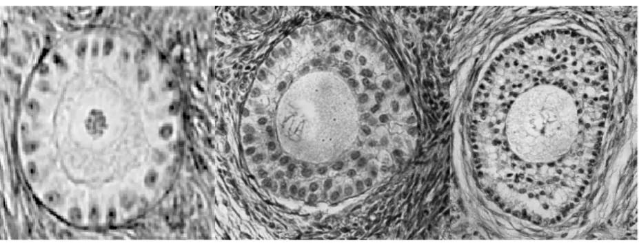
4.2.1. Biological background. The ovarian follicles are the basic anatomical and functional units of the ovaries. Structurally, an ovarian follicle is composed of a germ cell, named oocyte, surrounded by somatic cells (see Figure 5). In the first stages of their development, ovarian follicles grow in a compact way, due to the proliferation of somatic cells and their organization into successive concentric layers starting from one layer at growth initiation up to four layers.
Fig. 5. Histological sections of ovarian follicles in the compact growth phase. Left panel, one-layer follicle; center panel, three-one-layer follicle; right panel, four-one-layer follicle. Illustration courtesy of Danielle Monniaux.
4.2.2. Dataset description. We made use of a dataset providing us with mor-phological information at different development stages (oocyte and follicle diameter, total number of cells), acquired from ex vivo measurements in a sheep fetus [5]. In addition, from [14, 13], we can infer the transit times between these stages: it takes 15 days to go from one to three layers and 10 days from three to four layers. Hence (see Table 1(a)), the dataset consists of the total numbers of somatic cells at three time points.
Table 1
Experimental dataset and estimated values of the parameters. Table 1(b). The estimated value of \alpha and the initial number of cells are \alpha = 1.633 and N \approx 155, respectively. For j \geq 2, the bj parameter values (in blue) were computed using formula (9). The \lambda j values were computed
using formula (52). The 95\%-confidence intervals are b1 \in [0.0760; 0.1528], \alpha \in [0.0231; 5.685],
N \in [126.4; 185.4], p(1)S \in [0.6394; 0.7643], p(2)S \in (0; 0.7914], and p(3)S \in [0.6675; 0.9739]. (Table is in color online.)
(a) Summary of the dataset t = 0 t = 20 t = 35 Data points (62) 34 10 18 Total cell number 113.89 \pm 885.75 \pm 2241.75 \pm
57.76 380.89 786.26 Oocyte diameter 49.31 \pm 75.94 \pm 88.08 \pm (\mu m) 8.15 10.89 7.43 Follicle diameter 71.68 \pm 141.59 \pm 195.36 \pm (\mu m) 13.36 17.11 23.95
(b) Estimated values of the parame-ters. Layer j p(j)S bj \lambda j 1 0.6806 0.1146 0.0414 2 0.4837 0.0435 -0.0014 3 0.9025 0.0354 0.0285 4 1 0.0324 0.0324
We next take advantage of the spheroidal geometry and compact structure of ovarian follicles to obtain the number of somatic cells in each layer. Spherical cells are distributed around a spherical oocyte by filling identical width layers one after another, starting from the layer closest to the oocyte. Knowing the oocyte and somatic cell diameter (dOand ds, respectively) and the total number of cells Nexp, we compute
the number of cells on the jth layer according to the ratio between its volume Vjand
the volume of a somatic cell Vs:
Initialization: j \leftarrow 1, Vs\leftarrow \pi d
3 s 6 , N \leftarrow N exp While N > 0 : Vj\leftarrow \pi
6\bigl[ (dO+ 2 \ast j \ast ds) 3 - (d O+ 2 \ast (j - 1) \ast ds)3 \bigr] Nj\leftarrow min(V j Vs, N ), N \leftarrow N - Nj, j \leftarrow j + 1 J \leftarrow j - 1
The corresponding dataset is shown in the four panels of Figure 2.
4.2.3. Parameter estimation. Before performing parameter estimation, we take into account additional biological specifications on the division rates. The oocyte produces growth factors whose diffusion leads to a decreasing gradient of proliferating chemical signals along the concentric layers, which results in a recurrence law (9) sim-ilar to that initially proposed in [1]. Considering a regression model with an additive Gaussian noise, we estimate the model parameters to fit the changes in cell numbers in each layer (see SM1.2 in the supplementary material for details). The estimated parameters are provided in Table 1(b) and the fitting curves are shown in Figure 2. We compute the profile likelihood estimates [11] and observe that all parameters are practically identifiable except p(2)S (Figure SM1(a) in the supplementary material). In contrast, when we perform the same estimation procedure on the total cell numbers, most of the parameters are not practicality identifiable (dataset in Table 1(a); see detailed explanations in SM1.2 in the supplementary material).
5. Conclusion. In this work, we have analyzed a multitype age-dependent model for cell populations subject to unidirectional motion in both a stochastic and deter-ministic framework. Despite the nonapplicability of either the Perron--Frobenius or Krein--Rutman theorem, we have taken advantage of the asymmetric transitions be-tween different types to characterize long time behavior as an exponential Malthus growth, and obtain explicit analytical formulas for the asymptotic cell number mo-ments and stable age distribution. We have illustrated our results numerically, and studied the influence of the parameters on the asymptotic proportion of cells, Malthus parameter, and stable age distribution. We have applied our results to a morphody-namic process occurring during the development of ovarian follicles. The fitting of the model outputs to biological experimental data has enabled us to represent the compact phase of follicle growth. Thanks to the flexibility gained by the expression of morphodynamic laws in the model, we intend to consider other noncompact growth stages.
Acknowledgments. We thank Ken McNatty for sharing the experimental dataset and Danielle Monniaux for helpful discussions.
REFERENCES
[1] F. Cl\'ement, P. Michel, D. Monniaux, and T. Stiehl, Coupled somatic cell kinetics and germ cell growth: Multiscale model-based insight on ovarian follicular development, Multiscale Model. Simul., 11 (2013), pp. 719--746, https://doi.org/10.1137/120897249.
[2] T. E. Harris, The Theory of Branching Processes, Springer-Verlag, Berlin 1963.
[3] P. Jagers and F. C. Klebaner, Population-size-dependent and age-dependent branching processes, Stochastic Process. Appl., 87 (2000), pp. 235--254, https://doi.org/10.1016/ S0304-4149(99)00111-8.
[4] F. C. Klebaner, Introduction to Stochastic Calculus with Applications, 3rd ed., Imperial College Press, London, UK, 2012.