A Time-Scale Decomposition-Based Simulation Tool for Voltage Stability Analysis

(1)

Paper accepted for presentation at PPT 2001 2001 IEEE Porto Power Tech Conference

-131h September, Porto, Portugal

A Time-Scale Decomposition-Based Simulation

Tool for Voltage Stability Analysis

L. Loud

P. Rousseaux

D. Lefebvre

T. Van Cutsem

Absrruct-This paper proposes a time domain simulation tool combin-

ing Full Time Scale (FTS) simulation in the short-term period following a contingency and Quasi Steady-State (QSS) approximation for the long- term phase. A criterion is devised to automatically switch from FTS to QSS simulation as soon as sufficient damping of short-term dynamics is reached. Various comparisons with FTS simulations have been performed on the Hydro-Qn6bec system. The proposed method is shown to combine accuracy of FTS with computational efficiency of QSS. Sensitivity of sim- ulations to load model and the need for updating the whole model with frequency variations are also discussed.

K e y w r h - Quasi steady-state approximation, time domain simulation, voltage security analysis, voltage stability.

I .

INTRODUCTION

HE

need to perform detailed stability studies for various

T

system conditions is continuously increasing. Among the various stability problems that can be encountered, voltage instability is one of the most prominent. In power systems, it is customary to classify voltage dynamics in different time scales, from instantaneous to long-term 111, [2].

The short-term and instantaneous dynamics are usually represented by the differential/algebraic equations :

Equations ( 1 ) are the network relationships. They include the vector y of bus voltage magnitudes and phases. The short-term (or transient) dynamics of generators, SVCs, HVDC components, etc. are modeled by (2) with x the vector of corresponding short-term state variables.

The long-term dynamics are conveniently represented by mixed continuous / discrete-time equations :

where z, (resp. zd) is the continuous (resp. discrete) long-term state vector. Equation (4) captures the discrete transitions im- posed by control, protecting and limiting devices such as Load Tap Changers (LTC), automatic Shunt Reactor Trippings (SRT) or Overexcitation Limiters (OXL). In the sequel, we will refer to these devices as automata. An automaton undergoes transitions according to some logic; this occurs most often after a

L. Loud ([email protected]) is with the Research Institute of Hydro-QuCbec (IREQ), I800 Bvd Lionel-Boulet, Varennes (QC), Canada.

P. Rousseaux ([email protected]) and T. Van Cutsem ([email protected]) are with the department of Electrical Engi- neering (Institut Montefiore) o f the University of Likge, Sart Tilman, B28, E-4000 Likge, Belgium.

T. Van Cutsem is a research director of the F.N.R.S.

D. Lefebvre ([email protected]) is with the TransEnergie Division of

Hydro-Quibec, CP 10000 Montrial (QC), Canada.

0-7803-7139-9/01/$10.00 02001 TEEE

delay which may be constant, obey an inverse time characteris- tic or even be zero. Secondary frequency and voltage controls may yield both discrete (4) and continuous (3) equations. The differential equations (3) also stem from generic models of load recovery.

Within the context of voltage security assessment, time domain simulations are commonly used by industry. Unlike static tools such as conventional or continuation power flows, these time simulations do not suffer from modelling restrictions. The numerical integration of the whole set of equations (1)-(4) is referred to as Full Time Scale (FTS) simulation. Despite the in- crease in computer power and the development of efficient variable step size algorithms [3], FTS simulation remains a heavy approach.

Fast simulation tools have been derived from the Quasi Steady-State (QSS) approximation [4], [5

1.

In this approach, the short-term dynamics are supposed infinitely fast so that the corresponding differential equations (2) can be replaced by their equilibrium form :

In practice a reduced, equivalent set of equilibrium equations is handled. For instance, the representation of the generator and its regulators includes three x variables : the rotor angle

6,

the e.m.f.

E,

proportional to the field current and the e.m.f. E: behind saturated reactances [2].

By neglecting the short-term phenomena, this approach can deal with long-term voltage instability scenarios, the most fre- quently encountered type of voltage instability. However, in case of a severe contingency, the system may lose stability in the short-term time frame and hence not enter the long-term phase simulated by the QSS approximation. Moreover, even though transient angle and voltage instability phenomena most generally take place under different operating conditions and appear in distinct regions, some contingencies may lead to one or the other instability. Finally, controls acting in the first instants after a contingency can also have a major influence on the system long-term evolution. In this case, however, the initial conditions of a QSS simulation cannot be guessed without simulating the short-term phase.

In this paper we propose a coupled FTS-QSS simulation procedure. The objective

is

to devise

a

time domain tool combining accuracy and reliability of FTS simulation with computing efficiency of QSS approximation. The FTS simulation is used to simulate the short-term time period following the contingency. In case of short-term instability, the simulation stops. Other- wise, as soon as the short-term dynamics have died out, the simulation switches to the QSS approximation. The appropriate time to switch is chosen automatically, by observing damping

(2)

of short-term variables. Computational efficiency is obtained by limiting as much as possible the time interval handled by FTS.

Within the context of the FTS-QSS coupling, the impact of frequency excursions can be important. In

FTS

simulation, network parameters, such as line and machine reactances, can be continuously refreshed to track the slow frequency oscillations. On the other hand, the QSS approximation usually assumes constant reactances for the whole simulation. This paper also ex- plores how frequency variations echoed in network parameters can influence the overall system behavior.

The proposed method has been jointly developed by the Uni- versity of Liitge, Hydro-QuCbec and IREQ. It is intended to complement the QSS simulation implemented in the ASTRE software [ 5 ] ,

[6],

presently used at Hydro-Quebec in operational planning and evaluated for real-time applications.

The proposed method is described in Section I1 whereas il- lustrative results obtained on the Hydro-QuCbec system are reported in Section 111. Conclusions are offered in Section

IV.

11. C O U P L E D FTS-QSS SIMULATION TOOL

A. Outline of the procedure

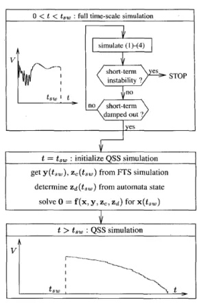
The proposed simulation procedure is sketched in Fig. 1. It consists of the following three steps.

1. FTS simulation is used to compute the system behavior in the first period following the contingency. This simulation phase takes into account both short-term and long-term dynamics.

(a) The simulation is checked to detect possible short-term instability, e.g. loss of synchronism or short-term voltage instability; if such an instability is detected, the simulation stops.

(b) Otherwise, the short-term dynamics are stable and the corresponding short-term variables x exhibit damped oscillations which eventually die out. When sufficient damping is reached, the FTS simulation stops. Let

t,,

be the corresponding time instant.

2. The short-term dynamics are thus assumed at equilibrium and the QSS approximation is used. To this purpose, the QSS model is initialized as described in section 1I.B.

3 . The rest of the simulation resorts to QSS approximation only. Note that this procedure is general : it can be built on any FTS

simulation tool, including as detailed modelling as desired. It may happen that, under the effect of a long-term instability, the evolution of long-term variables results in an instability of

the short-term dynamics. In such a case, the underlying assump- tion of the QSS approach breaks down. This may correspond to

[21 :

a loss of short-term equilibrium, resulting in loss of synchronism or motor stalling. This appears in QSS simulation as a singularity. In practice, (1,3,4,5) can no longer be solved and Newton iterations diverge;

an oscillatory instability of the short-term dynamics. This cannot be detected by QSS simulation. An eigenanalysis of the short-term Jacobian at points of the QSS long-term trajectory would be required 171.

The option of switching back to FTS simulation has not been investigated since, according to our experience, the above insta- bilities occur in clearly degraded system conditions. Even the detailed FTS model may be questionable in such circumstances !

t

0

<

t

<

taw : full time-scale simulation

-

vpj

t s w

'

t

L

J/

simulate (1)-(4) yes I

t = taw : initialize Q S S simulation get y ( t s w ) , z,(t,,) from FTS simulation

determine z d ( t s w ) from automata state solve 0 = f(x, y, z , , z d ) for x(t,,)

I

t

>

t s , : Q S S simulation

>

~~

Fig. 1. Coupled FTS-QSS simulation procedure

B. Switching from FTS to QSS simulation

In the first time instants following a disturbance, the system evolution is mainly dictated by the electromechanical oscillations between machines. This lasts typically for a few seconds and, if the system is short-term stable, results in a uniform system frequency. These fast oscillations are generally followed by slower oscillations of the system frequency which can thus be classified as a long-term variable. At this point, two options are possible : (i) either include in the QSS model the essential components responsible for these oscillations; (ii) or limit the QSS model to voltage phenomena and, consequently, wait for the frequency oscillations to die out before switching to QSS simulation. This paper concentrates on the second option.

Frequency oscillations are particularly visible in isolated systems such as the one used in this work. In large interconnected systems, on the other hand, frequency is expected to experience much smaller deviations. Hence, depending on the system char- acteristics,

t,,

can be fixed by observing the rotor angles or the system frequency oscillations.

For the Hydro-QuCbec system, for example, the devised switching criterion relies on the system frequency, as follows :

the successive extrema of the frequency signal are picked up during the FTS simulation process;

frequency damping is assessed on the basis of the last three successive extrema and switching is decided once damping has reached an acceptable value;

switching takes place when frequency passes through an es- timate of its final value. To this purpose, the time difference

(3)

between the two last extrema is taken as a good approximation of one half period of frequency oscillations; hence, one quarter of a period after the last extremum, frequency should be close to its final. This time is taken as

t,,.

Variables of the QSS simulation have to be carefully initialized at the switching time

t,,,

in particular long-term variables

z ,

and Z d . Although the time period from

t

= 0 to

t,,

is mainly dictated by short-term dynamics, the long-term variables cannot generally be considered constant during this period since the corresponding dynamics have already started to act. Con- sequently, the

QSS

model has to be initialized out of long-term equilibrium. This differs from a “pure” QSS simulation where all variables are initialized from a load flow calculation, assum- ing the system at both short and long-term equilibrium.

The continuous long-term variables z , and the algebraic variables y are simply set to the final values

z,(t,,)

and y(ts,) computed by FTS simulation. The QSS simulation uses

zc(ts,)

as initial conditions of the differential equations (3). Handling of discrete equations (4) is a bit less trivial since

t

does not necessarily coincide with automata discrete transition time. Moreover, an automaton may be waiting for transition when switching takes place. Consider for instance the case of

an OXL which can be in one of the following states : “idle” : the field current is below its threshold value; “waiting”: the current is above its threshold but the maximum overload time has not been reached yet;

“already acted” : field current is presently limited.

At

t,,,

FTS simulation has to communicate the state and, if in waiting state, the time elapsed since the OXL switched from idle to waiting. From there on, the initial conditions Z d ( t s w ) can be determined.

Finally, short-term variables are initialized using the QSS approximation. Since, on one hand, the QSS model relies on a reduced set of short-term variables and, on the other hand, these variables are not strictly at equilibrium at the end of the FTS

simulation, x(t,,) is obtained by solving

in which y,

z ,

and z d are set to the above discussed values.

111. RESULTS O N THE H Y D R O - Q U ~ B E C SYSTEM A . Voltuge stubility of the Hydro-QuCbec system

The Hydro-Quebec system

is

characterized by long distances (more than 1000 km) between the northern large hydro generation areas (James Bay, Churchill Falls and Manic-Outardes) and the southern main load center (around Montrial and Qutbec City). Accordingly, the company has developed an extensive 735-kV transmission system, whose lines are located along two main axes, the James Bay axis being complemented by a bipolar HVDC link. This system is angle stability limited in the North, voltage stability limited in the South. Frequency stability is also a concern due to the system interconnection through DC links only, as well as the sensitivity of loads to voltage. The peak load is around 35,000 MW.

Due to remote location of power plants, voltage is mainly con- trolled by SVCs and Synchronous Condensers (SCs). At peak load however, the total reactive reserve of compensators is not

sufficient to insure voltage stability following the most severe disturbances. For this reason, SRT devices were implemented

[8]. In operation since 1997, they are now available in 22 735- kV substations and control a large part of the total 25,500 Mvar shunt compensation. Each device relies on the local 735-kV bus voltage to switch reactors on or off, the coordination between substations being performed through the switching delays. While fast-acting SRT can improve transient angle stability, slower SRT significantly contributes to voltage stability.

B. Simulation tools and models

The simulations reported hereafter combine the Hydro- Quebec ST600 software [9], [IO] for FTS simulation and the ASTRE program [2], [6] developed by the University of LEge for long-term QSS simulation.

ST600 can simulate short and long-term dynamics, using si- multaneous implicit integration with fixed step size. It is also used as a benchmark for comparing accuracy. For coupling pur- poses, ASTRE has been provided with an interface which reads data in the ST600 load flow and dynamic data files and sets the initial conditions of the QSS simulation at the end of the ST600 process. The switching criterion, explained in Section ILB, is implemented in ST600 to automatically stop the simulation and output the relevant information to the interface.

The time steps adopted are 0.5 cycle, i.e. about 8 ms, in ST600 and 1 s in ASTRE.

The system modelling is the following.

Network : 661 buses at various levels from 735 to 120 kV, 859 lines and transformers. The dependency of loads with respect to voltage V and frequency deviations

A

f is modelled as follows :

P

= PO ( g ) ” ( l + K r A f T ) (7)

Q

=

Qo

(3

-

( ~ + K Q A ~ T )

(8)

where

PO,

Qo, VO refer to the initial load flow conditions. Pa- rameters of the above models are fixed as follows : a = 1.3, /3 = 2, K p =

0.7,

KQ

=

0.

In ASTRE, sensitivity to frequency has not been considered

( K p

= 0,

KQ

= 0).

ST600 continuously refreshes the line and generator reactances according to the actual frequency, while ASTRE consid- ers constant reactances, equal to their values provided by ST600 at the switching time

ts,.

Short-term dynamics : 1 1 SVCs, 85 generators and 9 SCs. In ST600, each generator or SC is represented by a 3-winding Park model, along with its turbine, governor, AVR and power system stabilizer. In ASTRE, each generator or SC is represented by three equilibrium equations (5). In each SVC, a zero- delay automaton limits the shunt susceptance.

Long-term dynumics : under- and overexcitation limiters on the synchronous condensers, SRT devices at eleven 735-kV substations with various short and long delays, 25 1 LTCs with various initial and subsequent delays.

C. Case studies

We consider two severe contingencies affecting the James Bay corridor : (i) tripping of the bipolar HVDC link; (ii) double-

(4)

... .,

...

~ original simulation 0.85 ... ,

~/

.\ : conitant reactjnces : , \ ; : \ : ~ \ , : 1 : : 1 : ' I '

-

... \ ... I I I I I I : 0.8 I I I 1 1 0 SO 100 IS0 200 250 300 t (s)

Fig. 2. Voltage computed by FTS simulation

line outage in the South part of the corridor. As the DC and the AC systems operate synchronously in the considered configura- tion, the first contingency results in a 2000 MW inrush in the AC lines of the corridor. The second contingency, on the other hand, suddenly increases the electrical distance between generation and load areas.

In the first time instants following such severe contingencies, voltages undergo a deep sag. During this period, SRT devices with short delays play an important role in preserving the system from short-term instability. Even if the system survives this period, long-term voltage instability may occur and, in turn, the long-term evolution is strongly influenced by SRT. As illustrated in the sequel, the number of SRTs triggered in the short-term period highly depends on the deepness of the initial voltage sag.

Moreover, correction of line and generator reactances according to frequency variations also influences the simulated behavior. This property is explored in Section 1II.C. 1 below by comparing FTS simulations with and without updating reactances. C.l Tripping of HVDC link

Fig. 2 shows the evolution of the voltage magnitude at a 735- kV bus in the Montrtal area, as computed by FTS simulation. The initial voltage sag induces the automatic tripping of 10 reactors during the 13 s following the contingency. This allows voltages to rapidly recover to normal values and avoids short- term instability. The system then enters the intermediate period between short-term and long-term and voltage variations follow the system frequency oscillations. Eventually, a long-term voltage collapse is encountered despite the tripping of one more reactor at 150 s.

Fig. 3 shows that the system can be stabilized by adding two slow SRT devices acting at 90 and 92 s respectively.

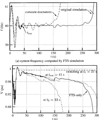
The evolution of system frequency corresponding to the case of Fig. 2 is drawn in Fig. 4.a. Three possible time instants to switch from FTS to QSS simulation are indicated by dots :

tl

= 21 s, t 2 = 33 s and

t,,

= 41 s, corresponding to increas-

ing damping. At each point, the frequency is close to the value at which it will settle down later on. The black dot refers to

t,,,

the time instant identified by the criterion of Section 1I.B.

The corresponding coupled FTS-QSS simulations are compared in Fig. 4.b. These curves confirm that QSS approximation is valid as soon as sufficient frequency damping is reached, while switching too early can lead to a misleading diagnosis. The re-

61 60 'c 59 ,

-

. . . I I I I I 0 SO 100 150 200 250 300 t (s)

(a) system frequency computed by FTS simulation

0 SO 100 IS0 200 250 300

t (SI

(b) voltage computed by FTS-only and coupled FTS-QSS simulations Fig. 4. Influence of switching instant

sult corresponding to

t,,

is very close to the original FTS simulation.

The key point of the proposed procedure is thus the choice oft,, : neither too early before short-term dynamics have died out, nor too late to preserve computational efficiency.

Fig. 5 compares the output given respectively by the FTS and the coupled FTS-QSS approaches in the stable case of Fig 3 .

The coupled FTS-QSS procedure is again in perfect agreement with the FTS simulation.

Figs. 2 , 3 and 4.a also compare the original FTS simulations with the simulations obtained by freezing line and generator re- actances at their initial load flow values. As can be observed in particular in Fig. 4.a, frequency oscillations have lower magnitudes when keeping reactances constant. However, the corresponding simulation is more severe. This apparent contradiction

(5)

a e

>

h v I 0.88 I I I I I 0 SO 100 IS0 200 2.50 300 a e

>

h v "."" 0 SO 100 IS0 200 2.50 300 t ( 5 )

Fig. 5. Stable case o f Fig. 3 : coupled FTS-QSS and FTS-only simulations

"."

0

so

100 IS0 200 2.50 300

t (SI

Fig. 6 . Coupled lTS-QSS simulations with constant reactances

can be explained as follows. If the initial frequency rise, and hence the voltage decrease, is less pronounced, a smaller number of fast SRT (6 instead of 10 in the reported cases) are needed to restore short-term equilibrium; also, voltages are restored but at lower values. The triggered devices have smaller delays; the remaining ones are reset

so

that, if voltages further fall down, they will possibly act too late for the system to be stable. Fig. 3 shows that the simulation diagnosis can be erroneous when using constant reactances throughout the simulation.

The coupled FTS-QSS simulations corresponding to the three switching times of Fig. 4.b are shown in Fig. 6 . The reactances are constant and identical in all simulations. Clearly, the QSS

part of the coupled simulations is much less sensitive to the switching time and reveals long-term instability as FTS simulation (although at a faster rate).

Initialization of frequency in the QSS simulation has thus a major influence on the method accuracy. In fact, electrical distances between generation and load areas depend directly on reactances and thus also on frequency when reactances are refreshed. Since the QSS simulation used in this paper does not model frequency oscillations, it is mandatory, in case of refreshed reactances, to wait for the oscillations to die out before switching. This guarantees an adequate initial frequency for the

QSS simulation. Using a too low (resp. too high) initial frequency provides optimistic (resp. pessimistic) initial conditions. In this respect, the situations considered in this study, namely an isolated system characterized by important initial frequency oscillations not modelled in QSS simulation, make up a set of stringent tests. I 0.95 h

z

;

0.9 0.85 n n "." 0 50 100 150 200 250 300 t (s)

Fig. 7. Coupled FTS-QSS and WS-only simulations (1st case)

I L ...

x

... : : .... ...

r

..., 7 ~~ 0.95 h P, 0.9 0.85 0.8 0 SO 100 150 200 250 t (s)

Fig. 8. Coupled FTS-QSS and FTS-only simulations (2nd case) 0

C.2 Double-line outage

The

a

and K p parameters of the load model (7) can have a major influence on the initial system oscillations. Simula- tions obtained for various ( a , K p ) pairs are gathered in Figs. 7

to 10. In these simulations, reactances have been updated with frequency.

As expected, in the very first instants after the contingency, increasing a! or decreasing K p has a beneficial effect. But in the

following period, the system may behave in the opposite way : larger

a

(resp. smaller K p ) give rise to smaller oscillations so

that eventually, it may happen than the initial ranking of simulations is reversed, as can be seen by comparing Figs. 7 and 8

(resp. Figs. 9 and IO). This property is mainly linked to SRT

as discussed in the previous section. Table I gathers the number of SRT devices triggered in the first 15 s of the simulation and confirms this observation.

TABLE 1

N U M B E R OF SRT DEVICES 1'KIGGERED I N T H E FIRST 1s S

CY K p Nb. OfSRTs

1.3 0.7 9

1.6 0.7 6

1.3 1 8

1.3

1.5 10

The FTS-QSS coupling procedure provides the dashed curves in Figs. 7 to 10. In each case, the agreement with FI'S simulation is very good. Note that in case of short-term instability (a! = l),

(6)

0.8 I I I I

’.

1

0 5 0 100 150 200 250 300

t 6)

Fig. 9. Coupled FTS-QSS and FTS-only simulations (3rd case)

t (s)

Fig. IO. Coupled FTS-QSS and FTS-only simulations (4th case)

the QSS part is not used. D. Coinputing times

Table I1 gives CPU times relative to three representative cases : (1) the long-term unstable scenario of Fig. 2; (2) the stable scenario of Fig. 3; (3) the short-term unstable scenario of Fig. 7. These results confirm the computational efficiency of the proposed coupled FTS-QSS method. Of course, the gain with respect to FTS simulation strongly depends on the switching time

tSw.

The gains shown in Table

I1

can be considered as

lower bounds. Indeed, the treated contingencies are severe ones and frequency oscillations take a rather long time to die out. In case of milder contingencies, switching to QSS could take place earlier, e.g. around 20 s.

TABLE I1

REPRESENTATIVECPU TIMES (S)

FTS simulation Coupled FTS-QSS procedure

FTS QSS

(1) 1243 290 2

(2) 1525

289

1.5

( 3 ) 125 125

IV. CONCLUSIONS

The simulation tool proposed in this paper exploits a time scale decomposition naturally present in power system stability problems. According to this approach, the short-term period is

computed with detailed integration while long-term simulation relies on the QSS approximation.

The switching from FTS to QSS simulation takes place automatically once the system exhibits enough damping of rotor angles or frequency swings. The successive extrema of angles or frequency curves arc used to this purpose. The choice between rotor angles or frequency is dictated by : (i) the existence of important frequency oscillations in the first part of the simulation; (ii) the modelling of these oscillations in the QSS simulation. In case of important frequency excursions and if the latter are not modelled in the QSS simulation, switching must take place after sufficient damping of frequency. Otherwise, it can be triggered earlier, once rotor oscillations have died out.

By limiting the period simulated by FTS as much as possible, the method achieves a good compromise between computational efficiency and accuracy.

From the user viewpoint, switching from one simulation program to the other is totally transparent since decision is taken by the program itself.

Moreover, any detailed simulation software can be used as

long as it can provide the information needed for QSS initialization out of equilibrium.

The method is able to deal with many types of stability problems, from short-term to long-term voltage instability. It has been shown to be well suited to the simulation of severe disturbances where short-term dynamics right after the contingency have a major influence on the long-term system evolution.

The switching criterion is likely to apply to many systems. In this respect, the tests performed on the Hydro-QuCbec system were severe and hence, the successful results obtained validate the proposed approach.

REFERENCES

C . W. Taylor, Power Sysrem Voltage Stabiliry McCraw Hill, EPRI Power System Engineering series, 1994.

T. Van Cutsem, C. Vournas, Voltage Stabiliry of Electric Power S y s t e m

Boston, Kluwer Academic Publishers, 1998.

M. Stubbe, A. Bihain, J. D e u x and J.C. Bauder, “STAG - A new uni- fied software program for the study of the dynamic behaviour of electrical power systems”, IEEE Trans. on Power Systems, vol. 4, pp. 129- 138, Feb.

1989.

A. Kurita, H. Okubo, K. Oki, S . Ageniatsu, D.B. Klapper, N.W. Miller, W.W. Price, J.J. Sanchez-Gasca, K.A. Wirgau and T.D. Younkins, “Multi- ple time-scale power system dynamic simulation”, IEEE Trans. on Power Systerns, vol. 8 , pp. 216-223, Feb. 1993.

T. Van Cutsem, Y. Jacquemart, J.-N. Marquet and P. Pruvot, “A compre- hensive analysis of mid-term voltage stability”, lEEE Trans. on Power

Systems, vol. 10, pp, 1173-1 182, Aug. 1995.

T. Van Cutsem and R . Mailhot, “Validation of a fast voltage stability analy- sis method on the Hydro-QuCbec system”, IEEE Trans. on Power Sysfenis,

vol. 12, pp. 282-292, Feb. 1997.

T. Van Cutsem, C. Vournas, “Voltage stability analysis in the transient and mid-term time scales”, lEEE Trans. on Power Sy.stems, vol. 1 I, pp.

146- 154, Feb. 1996.

S. Bernard, G. Trudel, G. Scott, “A 735-kV shunt reactors automatic switching system for Hydro-QuCbec network” IEEE Trans. on Power Sys-

fenis, vol. 11, pp. 2024-2030, Nov. 1996.

A. Valette, J . Huang and L. Loud, “ST600 Programme de stabilitC : manuel d’utilisation version 5.2”, Technical Report, Hydro-QuCbec, Direction principale recherche et diveloppement - IREQ, 2000.

R. Mailhot, “Voltage stability : impacts on Hydro-Quibec operations and simulation tools developments”, Proc. 3rd international workshop on Bulk’

power system voltage phenomena - voltage stability and security, Davos, Switzerland, Aug. 1994, pp. 207-213.