Sparsity Measure and the Detection of Significant Data

HAL Id: inria-00369628

https://hal.inria.fr/inria-00369628

Submitted on 20 Mar 2009

HAL is a multi-disciplinary open access

archive for the deposit and dissemination of

sci-entific research documents, whether they are

pub-lished or not. The documents may come from

teaching and research institutions in France or

abroad, or from public or private research centers.

L’archive ouverte pluridisciplinaire HAL, est

destinée au dépôt et à la diffusion de documents

scientifiques de niveau recherche, publiés ou non,

émanant des établissements d’enseignement et de

recherche français ou étrangers, des laboratoires

publics ou privés.

Sparsity Measure and the Detection of Significant Data

Abdourrahmane Atto, Dominique Pastor, Grégoire Mercier

To cite this version:

Abdourrahmane Atto, Dominique Pastor, Grégoire Mercier. Sparsity Measure and the Detection of

Significant Data. SPARS’09 - Signal Processing with Adaptive Sparse Structured Representations,

Inria Rennes - Bretagne Atlantique, Apr 2009, Saint Malo, France. �inria-00369628�

Sparsity Measure and the Detection of Significant Data

Abstract—The paper provides a formal description of the sparsity of

a representation via the detection thresholds. The formalism proposed derives from theoretical results about the detection of significant coefficients when data are observed in presence of additive white Gaussian noise. The detection thresholds depend on two parameters describing the sparsity degree for the representation of a signal. The standard universal and minimax thresholds correspond to detection thresholds associated with different sparsity degrees.

Index Terms—Sparsity measure, Wavelets, Detection thresholds.

I. INTRODUCTION

The detection thresholds are synthesized by considering a risk function which is the probability of erroneously deciding that a coefficient is significant when it is not the case. They depend on two parameters that can be used to bound the sparsity degree of the wavelet representation [1]. These thresholds are optimal in the sense that they lead to the same upper bound for the probability of error than the Bayes test with minimal probability of error among all possible tests [2], for a certain class of signals, including sparse signals. It is shown in this paper that the standard minimax and universal thresholds are detection thresholds corresponding to different degrees of sparsity. The selection of appropriate detection thresholds with respect to the wavelet decomposition properties of some signals such as smooth and piecewise regular signals is also discussed.

II. DETECTION THRESHOLDS ANDSPARSITY DEGREE

Consider the following decision problem with binary hypothesis model (H0,H1), where H0: ci∼ N (0, σ2) versusH1: ci= di+

²i, |di|> a> 0, ²i∼ N (0, σ2).

Letξ be the function defined for ρ > 0 and 06p61/2 by ξ(ρ,p) =ρ 2+ 1 ρ " ln1 − p p + ln à 1 + s 1 − p 2 (1 − p)2e−ρ 2 !# . (1)

Assume that the a priori probability of occurrence of hypothesis H1 is less than or equal to some value p∗61/2. Then, for

deciding H0 versus H1, the thresholding test with threshold

heightλD(a, p∗),

λD(a, p∗) = σξ(a/σ,p∗), (2)

has the same sharp upper bound for its probability of error than the Bayes test with the least probability of error (see [2] for details). Parameter p∗ reflects the presence (quantity) of significant coefficients of the signal amongst the noisy coefficients. Assuming that p∗is less than or equal to 1/2 ensures that the representation of the signal is at least sparse (in the weak sense).

Parameteracan be seen as the minimum amplitude considered to be significant for a signal coefficient. Parameters p∗andathus allow to formalize more precisely the sparsity degree of the signal representation (see [1]).

In what follows, we consider σ = 1 for the sake of simplicity. The following proposition unifies the minimax, universal, and detection thresholds.

1_{TELECOM Bretagne, am.atto@telecom-bretagne.eu} 2_{TELECOM Bretagne, dominique.pastor@telecom-bretagne.eu} 3_{TELECOM Bretagne, gregoire.mercier@telecom-bretagne.eu}

Proposition 1: For any positive real valueη, there exist a0> 0

and p₀∗, with 06p∗₀61/2, such that

λD(a0, p∗0) = η. (3)

Proof: The result simply follows by noting thatξ is continuous, positive, lim_p→0ξ(ρ,p) = 0 for fixed ρ > 0, and lim_ρ→+∞ξ(ρ,p) = +∞ for fixed p, 0 < p61/2.

Let λu(N ) = σ

p

2 ln N , the so-called universal threshold. This threshold reflects the maximum amplitude of the white Gaussian noise coefficients. Indeed, if²iiid∼N (0,σ2), it follows from [3, p. 187]; [4, p. 454], that lim N →+∞P · λu(N ) − αN6max n |²i| o 16i6N6λu(N ) ¸ = 1, (4) with αN = σ ln ln N /ln N . Thus, the maximum amplitude of

{²i}16i6N has a strong probability of being close to the universal

threshold when N is large.

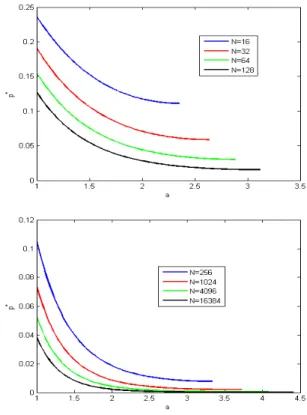
From proposition 1, it follows that for any N>2, there exist some values a, p∗ such that λD(a, p∗) = λu(N ). Figure 1 shows

the level curves λD(a, p∗) = λu(N ) for different values of N . It

appears that large values ofaare associated with small values of p∗ (strong sparsity) and vice versa (weak sparsity).

Fig. 1. Level curvesλD(a, p∗) = p

2 ln N for different values of N .

The same remark (as for the universal threshold) holds true for the minimax threshold. The minimax thresholdλm(N ) is defined

as the largest valueλ among the values attaining a minimax risk bound given in [5].

III. DETECTION OF SIGNIFICANT WAVELET COEFFICIENTS

Detection thresholds are well-adapted to estimate wavelet coef-ficients corrupted by AWGN because of the sparsity of the wavelet transform [2]. Moreover, these thresholds are adaptable to the wavelet transform decomposition schemes: sparsity ensures that for reasonable resolution levels, signal coefficients are less present than noise coefficients among the detail wavelet coefficients and that signal coefficients have large amplitudes (in comparison to noise coefficients).

More precisely, it is known that for smooth or piecewise regular signals, the proportion of significant coefficients, which plays a role similar to that of p∗, increases with the resolution level [4, Section 10.2.4, p. 460]. Therefore, if we can give, first, upper-bounds (p∗_j)_{j =1,2,···,J}; p∗_j 61/2 for every j = 1,2,··· , J, and second , lower-bounds (a_j)_{j =1,2,···,J} for the amplitudes of the significant wavelet coefficients, then we can derive level-dependent detection thresholds that can select significant wavelet coefficients at every resolution level. Since significant information tends to be absent among the first resolution level detail wavelet coefficients, it is reasonable to set a1= σ

p

2 ln N , that is the universal threshold. Now, when the resolution level increases, it follows from [4, The-orem 6.4] that a convenient choice foraj, j > 1 isaj=a1/

p 2j −1 when the signal of interest is smooth or piecewise regular.

In addition, since noise tends to be less present when the resolution level increases, p∗_j must be an increasing function of j . Note that detection thresholds are defined for p∗_j 61/2. It is thus essential to stop the shrinkage at a resolution level J for which p∗_J is less than or equal to 1/2. We propose the use of exponentially or geometrically increasing sequences for the values (p∗_j)_{j =1,2,···,J} since p₁∗ must be a very small value (significant information tends to be absent among the first resolution level detail wavelet coefficients) and the presence of significant information increases significantly as the resolution level increases. In the following, we consider a sequence (p∗_j)_{j =1,2,···,J} such that p∗_{j +1}= (p∗_j)1/µ with µ > 1.

Summarizing, we consider the thresholdsλD(aj, p∗_j), whereλD

is defined by Eq. (2) and (a_j, p∗_j), for j = 1,2,··· , J are given by

aj= σ

p

ln N /2j /2−1, (5) and

p∗_j = 1/2µJ −j. (6)

IV. DETECTION THRESHOLDS IN PRACTICE

Experimental tests are carried by using the Stationary Wavelet Transform (SWT) and the biorthogonal spline wavelet with order 3 for decomposition and with order 1 for reconstruction (‘bior1.3’ in Matlab Wavelet toolbox). The maximum decomposition level is fixed to J = 4. The SWT [6] has appreciable properties in denoising. Its redundancy makes it possible to reduce residual noise and some possible artifacts incurred by the translation sensitivity of the orthonormal wavelet transform.

The detection thresholds are used to calibrate the Smooth Sig-moid Based Shrinkage (SSBS) functions of [7]. The SSBS functions are smooth functions and they allow for a flexible control of the shrinkage through parameters which model the attenuation imposed to small, median and large data. This allows correcting the main drawbacks of the soft and hard shrinkage functions. The SSBS functions are defined by:

δt ,τ,λ(x) =sgn(x)(|x| − t)+

1 + e−τ(|x|−λ) , (7)

for x ∈ R, (t,τ,λ) ∈ R+×R∗+×R+, where sgn(x) = 1 (resp. -1) if x>0

(resp. x < 0), and (x)+= x (resp. 0) if x>0 (resp. x < 0).

The results below were obtained with the following values for the SSBS parameters. We consider the values

• t0= 0 and θ0= π/10 when the noise standard deviation σ is

less than or equal to 5,

• t0= σ/5 and θ0= π/6 when 5 < σ615,

• t0= σ/3 and θ0= π/5 when σ is larger than 15.

In addition, we use as threshold heights λ0( j ) = λD(aj, p∗_j), the

detection thresholds defined by Eq. (2), where (aj, p∗_j), for j =

1, 2, ··· , J are given by Eqs. (5) and (6). We use the value µ = 2.35 in Eq. (6), which tend to be a good compromise for the different test images used, and we assume that p∗_J= 1/2.

The PSNR (in deciBel unit, dB) is used to assess the quality of a denoised image,

PSNR = 10log10

³

2552/MSE´. (8) PSNRs achieved by SSBS are given for several values of the noise standard deviation in table I, in comparison to the BLS-GSM method of [8]. The latter (free MatLab software 1) is a parametric method using redundant wavelet transform and mod-els neighbourhoods of wavelet coefficients with Gaussian vectors multiplied by random positive scalars. BLS-GSM also takes into account the orientation and the interscale dependencies of the wavelet coefficients. It is actually the best parametric method using redundant wavelet transform and it is computationally expensive (see [9] for an appreciation of the BLS-GSM computing time).

According to table I, the performance of SSBS is comparable to that obtained with BLS-GSM in terms of PSNR. Indeed, the difference in PSNR between SSBS and BLS-GSM is about 1 dB, which can be regarded as a good result since SSBS is a simple non-parametric method (in the sense that neither interscale nor intra-scale predictors are included in the shrinkage process).

In addition, we now address the sensitivity of the SSBS cali-brated by the detection thresholds according to the wavelet filters. Table II presents the PSNRs obtained by using different filters. It follows from this table that, for a given wavelet family, there is no significant variability of the results with respect to the length of the wavelet filter used: short impulse response wavelet filters perform better with the ‘House’ image while long impulse response filters perform better with the ‘Fingerprint’ image. Thus, the best PSNR still depends on the input image. In addition, there is no significant difference between the results obtained with respect to the wavelet family used, when the length of the filters are sensibly of the same order.

V. CONCLUSION

This paper highlights some remarkable properties of the detec-tion thresholds. Detecdetec-tion thresholds depend on two parameters that describe the sparsity of the wavelet representation in terms of “minimum significant amplitude” for the signal and “probability of occurrence” of the significant signal coefficients in the sequence of wavelet coefficients. It is shown that the universal and minimax thresholds are particular detection thresholds corresponding to different degrees of sparsity.

On the other hand, this paper analyzes the combination be-tween detection thresholds and the SSBS functions. The SSBS functions are a family of smooth sigmoid based shrinkage func-tions which perform a penalized shrinkage. The experimental

TABLE I

MEANS AND VARIANCES OF THEPSNRS COMPUTED OVER25NOISE REALIZATIONS,WHEN DENOISING TEST IMAGES BY THESSBSANDBLS-GSMMETHODS. THE TESTED IMAGES ARE CORRUPTED BYAWGNWITH STANDARD DEVIATIONσ. THESWTIS COMPUTED BY USING THE SPLINE‘BIOR1.3’WAVELET. THESSBS

PARAMETERS(t0,θ0,λ0)GIVEN IN SECTIONIVARE USED.

Image ‘House’ ‘Peppers’ ‘Barbara’ ‘Lena’ ‘Fingerprint’ ‘Boat’

σ = 5 (=⇒ Input PSNR = 34.1514). Mean(PSNR) SSBS 37.9508 37.4567 35.8365 37.8641 35.2408 36.2997 BLS-GSM 38.2248 37.5750 37.1966 38.1847 36.3801 36.7190 Var(PSNR) ×1003 SSBS 0.6045 0.6371 0.2058 0.1528 0.0783 0.1244 BLS-GSM 0.0080 0.0028 0.0004 0.0004 0.0012 0.0008 σ = 15 (=⇒ Input PSNR = 24.6090). Mean(PSNR) SSBS 32.9988 31.5997 28.4616 32.8278 29.1183 30.8712 BLS-GSM 33.8043 32.0354 30.7868 33.4822 29.9361 31.6285 Var(PSNR) SSBS 0.0023 0.0016 0.0003 0.0007 0.0001 0.0004 BLS-GSM 0.0011 0.0027 0.0001 0.0002 0.0002 0.0002 σ = 25 (=⇒ Input PSNR = 20.1720). Mean(PSNR) SSBS 30.6291 28.6862 25.6226 30.5796 26.3489 28.4944 BLS-GSM 31.6253 29.4782 27.8179 31.2575 27.1177 29.2595 Var(PSNR) SSBS 0.0020 0.0024 0.0001 0.0005 0.0004 0.0006 BLS-GSM 0.0034 0.0070 0.0008 0.0004 0.0002 0.0005 σ = 35 (=⇒ Input PSNR = 17.2494). Mean(PSNR) SSBS 29.0606 26.6922 24.4933 29.1528 24.6512 27.1420 BLS-GSM 30.0584 27.8208 25.9688 29.7596 25.2411 27.7355 Var(PSNR) SSBS 0.0043 0.0023 0.0002 0.0006 0.0004 0.0006 BLS-GSM 0.0037 0.0032 0.0006 0.0007 0.0004 0.0012 TABLE II

AVERAGEPSNRS COMPUTED OVER25NOISE REALIZATIONS,WHEN DENOISING TEST IMAGES BY THESSBSMETHOD. THE TESTED IMAGES ARE CORRUPTED BY

AWGNWITH STANDARD DEVIATIONσ = 35. THESWTIS COMPUTED BY USING DIFFERENTDAUBECHIES,SPLINE,AND SYMLET WAVELETS REFERENCED AS IN THEMATLABWAVELET TOOLBOX. THESSBSPARAMETERS(t0,θ0,λ0)GIVEN IN SECTIONIVARE USED.

Image ‘House’ ‘Peppers’ ‘Barbara’ ‘Lena’ ‘Fingerprint’ ‘Boat’

Daubechies filters ‘db1’ 28.6500 26.2633 24.1965 28.6561 23.1275 26.6957 ‘db2’ 28.2556 26.0992 24.3287 28.8418 24.3481 26.7808 ‘db4’ 28.0620 25.6922 24.4194 28.7922 24.8339 26.6889 ‘db8’ 27.5814 25.1000 24.3617 28.5160 24.8711 26.4323 Symlet filters ‘sym1’ 28.6889 26.2879 24.2026 28.6630 23.1335 26.6878 ‘sym2’ 28.2613 26.0705 24.3386 28.8387 24.3446 26.7780 ‘sym4’ 28.2320 25.9667 24.4539 28.9027 24.8237 26.7770 ‘sym8’ 28.0018 25.7022 24.4534 28.8234 24.9062 26.6888

Spline biorthogonal filters

‘bior1.1’ 28.6650 26.2695 24.1935 28.6614 23.1377 26.6907 ‘bior2.2’ 27.6983 25.7494 24.4346 28.2951 24.8211 26.6846 ‘bior4.4’ 28.0672 25.8622 24.4830 28.7680 24.6440 26.6894 ‘bior6.8’ 28.0400 25.7525 24.5354 28.8420 24.9629 26.7517

(a) Noisy image PSNR=17.25 dB (b) SSBS PSNR=27.1220 dB (c) BLS-GSM PSNR=27.7766 dB

Fig. 2. SSBS and BLS-GSM denoising of noisy ‘Boat’ image corrupted by AWGN with standard deviationσ = 35.

results show that SSBS functions adjusted with these detection thresholds achieve denoising PSNR comparable to that of the best parametric and computationally expensive method, the BLS-GSM of [8]. This performance is remarkable for a non-parametric method where no interscale or intra-scale predictors are used to provide information about significant wavelet coefficients.

REFERENCES

[1] D. Pastor and A. M. Atto, “Sparsity from binary hypothesis testing and application to non-parametric estimation,” European Signal Processing

Conference, EUSIPCO, Lausanne, Switzerland, August 25-29, 2008.

[2] A. M. Atto, D. Pastor, and G. Mercier, “Detection threshold for non-parametric estimation,” Signal, Image and Video Processing, Springer, vol. 2, no. 3, Sept. 2008.

[3] S. M. Berman, Sojourns and extremes of stochastic processes. Wadsworth and Brooks/Cole, 1992.

[4] S. Mallat, A wavelet tour of signal processing, second edition. Academic Press, 1999.

[5] D. L. Donoho and I. M. Johnstone, “Ideal spatial adaptation by wavelet shrinkage,” Biometrika, vol. 81, no. 3, pp. 425–455, Aug. 1994. [6] R. R. Coifman and D. L. Donoho, Translation invariant de-noising.

Lecture Notes in Statistics, 1995, no. 103, pp. 125–150.

[7] A. M. Atto, D. Pastor, and G. Mercier, “Smooth sigmoid wavelet shrink-age for non-parametric estimation,” IEEE International Conference on

Acoustics, Speech, and Signal Processing, ICASSP, Las Vegas, Nevada,

USA, 30 march - 4 april, 2008.

[8] J. Portilla, V. Strela, M. J. Wainwright, and E. P. Simoncelli, “Image denoising using scale mixtures of gaussians in the wavelet domain,”

IEEE Transactions on Image processing, vol. 12, no. 11, pp. 1338–1351,

November 2003.

[9] F. Luisier, T. Blu, and M. Unser, “A new sure approach to image denois-ing: Interscale orthonormal wavelet thresholding,” IEEE Transactions