HAL Id: hal-00473610
https://hal-mines-paristech.archives-ouvertes.fr/hal-00473610
Submitted on 12 May 2010
HAL is a multi-disciplinary open access
archive for the deposit and dissemination of
sci-entific research documents, whether they are
pub-lished or not. The documents may come from
teaching and research institutions in France or
abroad, or from public or private research centers.
L’archive ouverte pluridisciplinaire HAL, est
destinée au dépôt et à la diffusion de documents
scientifiques de niveau recherche, publiés ou non,
émanant des établissements d’enseignement et de
recherche français ou étrangers, des laboratoires
publics ou privés.
Iterative calibration method for inertial and magnetic
sensors
Eric Dorveaux, David Vissière, Alain Pierre Martin, Nicolas Petit
To cite this version:
Eric Dorveaux, David Vissière, Alain Pierre Martin, Nicolas Petit. Iterative calibration method for
inertial and magnetic sensors. 48th IEEE Conference on Decision and Control, Dec 2009, Shanghai,
China. pp.8296-8303, �10.1109/CDC.2009.5399503�. �hal-00473610�
Iterative calibration method for inertial and magnetic sensors
Eric Dorveaux, David Vissière, Alain-Pierre Martin, Nicolas Petit
Abstract— We address the problem of three-axis sensor cali-bration. Our focus is on magnetometers. Usual errors (misalign-ment, non-orthogonality, scale factors, biases) are accounted for. We consider a method where no specific calibration hardware is required. We solely use the fact that the norm of the sensed field must remain constant irrespective of the sensors orientation. The proposed algorithm is iterative. Its convergence is studied. Experiments conducted with MEMS sensors (magnetometers) stress the relevance of the approach.
INTRODUCTION
Numerous military and civilian control applications re-quire high accuracy position, speed, and attitude estimations of a solid body. Examples range from Unmanned Air Vehi-cles (UAV), Unmanned Ground VehiVehi-cles (UGV), full-sized submarines, civil engineering positioning devices, to name a few. A widely considered solution is to use embedded Inertial Measurement Units (IMU). Accelerometers, gyro-scopes signals can be used to derive position and orientation information through a double integration process [11], [7]. This approach requires very high precision IMUs and well calibrated sensors. An important challenge appears when cost, space or weight constraints become stringent.
The recent progress in very low cost (less than 300 USD), low weight (less than 100 g) and low size (less than 3 cm2) IMUs have spurred a broad interest in the development of IMU-based positioning technologies. These Micro-Electro-Mechanical Systems (MEMS) IMUs appear to have quickly increasing capabilities. Several manufacturers are announc-ing new models under 4,000 USD capable of less than 20 deg/hr angular errors.
Yet, there still does not exist any reported experiment proposing to estimate the position from such a low cost IMU. In the literature, these IMUs are only used for ori-entation (attitude) estimation (see e.g. [4], [12] or [3] for an application to the control of mini-UAVs in closed loop). Some tentative work (using higher-end IMUs) address the problem of velocities estimation. In these cases, the speed information is obtained from a GPS receiver using the Doppler effect (see [11] for details on the quality of the obtained measurements information) or from odometers (in
E. Dorveaux (corresponding author) is a PhD candidate in Mathematics and Control, Centre Automatique et Systèmes, Mines-ParisTech, 60, bd St Michel, 75272 Paris, France
D. Vissière is with SYSNAV, Zone industrielle B, 1 rue Jean de Becker Rémy, BP86, 27940 AUBEVOYE, France
A. P. Martin is “Ingénieur” in the Délégation Générale pour l’Armement (DGA) of the French Department of Defense.
N. Petit is with the Centre Automatique et Systèmes, Mines-ParisTech, 60, bd St Michel, 75272 Paris, France
the case of ground vehicles). Model based approaches permit to reduce the dependence on GPS (see [15]).
For indoor pedestrian applications, GPS is almost totally unavailable. Recently, a new approach called distributed-magnetic-inertial navigation has been proposed [16]. It re-lies solely on MEMS magnetometers, accelerometers and gyroscopes and takes advantage of the unknown magnetic field disturbances usually observed indoors to estimate drift in velocities. This disturbances are evaluated using a three-dimensional array of magnetometers. In details, an exper-imental test bed was constructed that integrates an IMU consisting of one three-axis accelerometer, one three-axis gyroscope and one three-axis magnetometer and a set of eight spatially distributed three-axis magnetometers. This complex measurement system can produce meaningful data if and only if all the sensors are well-calibrated and all the sampling times are precisely known and accounted for (this last point is discussed in [6]). Calibration of such three axis sensors measuring a constant vector field is the subject of this paper. In classic inertial navigation, there exist various methods for three-axis sensors calibration. Most of them have an important drawback in common. They require expansive tools to acquire the data and compare them against a fixed reference, and, quite often, a high degree of expertise to process the data. Usually (see e.g. [5]), IMUs calibration is achieved using a well-instrumented mechanical platform (called calibration table) whose varying orientation is pre-cisely measured. The platform is rotated to various prepre-cisely controlled orientations which serve as comparisons against the orientations determined from the IMU sensors. The rotational velocities are precisely controlled as well. Mag-netometers calibration is usually performed using a similar method in magnetically shielded facilities to provide a known uniform field (see e.g. [13]). Similarly, measurements are then performed with precise knowledge of sensors orienta-tion.
The recent development of micro-electro mechanical sys-tems (MEMS) and other low-cost sensors has led to a paradox. Due to their relatively low quality, these low-cost sensors are in great need of a calibration procedure (much more than higher-end sensors), but the cost of the traditional calibration procedures may exceeds by many times the cost of developing and constructing the sensors themselves, and calibration may change over time. Moreover, as the cost of the sensors are decreasing, their use is spreading. This yields a great interest in developing new "simple but effective" calibration procedures that do not require a high degree of expertise nor an expensive hardware to be put into practice. Lately, a new paradigm for such sensors calibration has
7)3$8)3#9&:;<;&,)#$39&1.0.=>./&?@A?(9&6BBC
emerged. Some procedures and algorithm have been pro-posed (see [14], [8]) and a few for magnetometers calibration (see [10], [9]). They all rely on the fact that the force field un-der consiun-deration (the gravitational field for accelerometers and the Earth magnetic field for magnetometers) corresponds to a sensed vector having, in theory, a constant and known norm. The strategy is to identify and remove the measure-ment errors. No specific calibration hardware is required.
The measurement errors are represented by constant co-efficients of a (vector) affine transformation. The calibra-tion problem is to find inverse affine transformacalibra-tions to maximize a performance index. This index involves the norm of the reconstructed data and a comparison against its theoretical (scalar) constant value. In practice, the usual algorithm (see [10], [9]) proceeds in two steps. First, an exact linearization is performed by means of a change of variables. Then, an inverse transformation is analytically (or numerically) performed to obtain the desired variables. Inter-estingly, the linearizing change of coordinates is not unique. Several choices are possible and all yield some distorsion in the cost function. For cases where the sensed field is possibly substantially distorted (such as the above mentioned indoor applications), irrelevant solutions can appear. They may correspond to cases where the cost function is also substantially distorted.
In this paper we propose to go back to an original nonlinear formulation, close in spirit with those considered in the calibration-table free methods (see [10], [9], [14], [8]), and to treat it in an iterative way. This yields an algorithm with interesting mathematical properties, which is also very efficient in practice. More specifically, we address the case of magnetometers which is of particular interest for the distributed magnetometry applications mentioned above, but the method has also been applied successfully to accelerometers.
The article is organized as follows. In Section I, the calibration problem is defined along with the mathematical model used. The main magnetic disturbances (hard-iron, soft-iron) are briefly recalled and modeled along with the classic scale factors and misalignments. Notations required for the study of the calibration algorithm are presented. We also briefly present the distributed magnetometry test bed experiments are conducted on. In Section II, the state-of-the-art non-linear two-steps estimation algorithm and the proposed method are described for sake of further compar-isons. In Section III, properties of the proposed algorithm are established. Experimental results are presented in Section IV. Finally, we conclude and sketch future directions.
I. CALIBRATIONPROBLEM
In this section, we expose the calibration problem for a three-axis sensor. We present an error model and the notations employed throughout the paper.
A. Notations
Consider a three-axis sensor. Its sampled measurements are denoted𝑦𝑖(3×1 vector), where 𝑖 stands for the sampling
index, whereas the actual value of the sensed field is denoted 𝑌𝑖 (3 × 1 vector). These measurements are collected in 𝑦 =
(𝑦𝑖)𝑖=1,...𝑁, where𝑁 is the total number of samples.
In order to improve the accuracy of raw sensor data 𝑦,
especially when dealing with low-cost sensors, mathematical models must be built to take into account the various sources of errors. Some, such as scale-factors, misalignment and the resulting cross-coupling of axes, apply to all kinds of sensors (gyroscopes, accelerometers, ...) while some others only apply to a particular class of sensor (see below for the case of magnetometers). To cover most cases of interest, we might
have simply considered a zero-bias vector 𝛽, scale-factors
represented by a diagonal matrix𝛼, and misalignments terms (accounting for harmonization errors only) represented by a
skew-symmetric matrix𝑅 𝑌𝑖 = 𝛼𝑅𝑦𝑖+ 𝛽 with 𝛽 = [𝛽1 𝛽2 𝛽3]𝑇 𝑅 = ⎡ ⎣ 1 𝜓 −𝜃 −𝜓 1 𝜙 𝜃 −𝜙 1 ⎤ ⎦𝛼 = ⎡ ⎣ 𝛼1 𝛼2 𝛼3 ⎤ ⎦
However, due to the use of low cost sensors, substantial mis-alignments and errors must be considered, and, additionally, significant non-orthogonality between axes may arise. There-fore, no possibly simplifying assumption on the magnitude of the errors is made. All these factors are gathered into
a general matrix 𝐴, and a zero-bias vector 𝐵. With these
notations,
𝑌𝑖= 𝐴𝑦𝑖+ 𝐵 (1)
In the case of magnetometers which is of particular interest here, the specific sources of errors are mainly hard and soft iron errors (see [10], [13]). Hard iron errors are induced by permanent unwanted fields. They are generated by ferromagnetic materials attached to the magnetometer frame (typically the structure or the equipment installed near the magnetometer, or even non-varying current in close-by wires). They result in a bias. Soft iron errors are induced by materials that generate magnetic fields in response to externally applied magnetic fields. The model presented in this paper takes only into account the proportionality of this error to the applied external field. The constant of proportionality is referred to as the magnetic susceptibility of the material considered. Soft iron errors generally present a hysteresis which is often small enough to be neglected.
Without any disturbances on the sensed field, the only information available is that the actual norm of the sensed field is constant during all the measurement acquisition phase. This constant may be chosen equal to 1 without any loss of generality1. The calibration problem consists in
determining 𝐴 and 𝐵 from the measurements 𝑦 knowing
that the actual norm of the sensed field 𝑌𝑖 is 1 for all
samples𝑖 = 1, ..., 𝑁 .
1This standpoint is different from numerous approaches found in the
literature [2] where the norm of the sensed field is obtained from dependable look-up tables. No such information is available indoor.
!"#$%&'
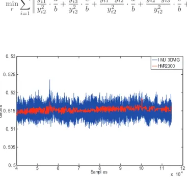
4 5 6 7 8 9 10 11 12 x 104 0. 48 0. 49 0. 5 0. 51 0. 52 0. 53 0. 54 0. 55 Sampl es Ga u s s I MU 3DMG HMR2300
Fig. 1. Norm of the magnetic field before calibration for two distinct magnetometers (one HMR2300 from HoneywellⓇand one included in the MicrostrainⓇIMU). The errors are due to the sensor ill-calibration.
B. Obtaining experimental data
Measurements are obtained while the three-axis sensor (magnetometer) is oriented in every possible direction. The motion is usually relatively slow, but this is not a strict requirement. Interestingly, no accurate measurements of the sensor orientation is made during this data acquisition. This makes the classically considered calibration table useless in this data collection step. The Earth magnetic field and the hard and soft iron errors are assumed constant during the data collection process. Similarly, for accelerometers calibration, the gravitational field would be also considered constant. To avoid any temperature drift, the sensors have to be warmed up before data acquisition. This warm-up phase last approximatively 1 min. The data acquisition phase lasts
approximatively 25 min and a typical number of 𝑁 = 105
samples are acquired. C. Experimental testbed
The experimental testbed used here is described in [6]. In summary, nine magnetometers (e.g. HMR2300 from HoneywellⓇ) are attached to a board which can simulta-neously rotate and translate in 3D. A MicrostrainⓇIMU is located in the center of the device. A power-PC microcon-troller (MPC555 from MotorolaⓇ) is used to retrieve the data from all sensors and associate a time-stamp to each measurement for sake of synchronization. The measurement from all the sensors are gathered along with their timestamps in a single message sent through a serial port to a remote computer for post-treatment. Before the calibration process is achieved, the norm of the sensed magnetic fields varies significantly (see Figure 1 where the norms of the𝑁 samples are plotted).
II. CALIBRATION METHODS
A. Non-linear, two-step estimation algorithm
Here, we briefly recall the two-step calibration algorithm originally proposed in [10], [9]. As the norm of the sensed
field is assumed constant ∥𝑌𝑖∥ 2
= 1, for all 𝑖 = 1, ..., 𝑁 ,
the sensed field vectors 𝑦𝑖 should all be located on the
unit sphere. Due to errors, this is not the case, as already
discussed. It is desired to find 𝐴 and 𝐵 such that the
values 𝐴 (𝑦𝑖− 𝐵) are as close as possible to this sphere.
In details, 𝐴 and 𝐵 have to yield a fair approximation of
∥𝐴 (𝑦𝑖− 𝐵)∥ 2
= 1 for every sample 𝑖 = 1, ..., 𝑁 . To this end,𝐴 and 𝐵 are defined as the minimizers of the following cost function (2) 𝑔 (𝐴, 𝐵, 𝑦) = 𝑁 ∑ 𝑖=1 ( ∥𝐴 (𝑦𝑖− 𝐵)∥ 2 − 1) 2 (2) Once expanded, it becomes
𝑔 (𝐴, 𝐵, 𝑦) = 𝑁 ∑ 𝑖=1 (𝑦𝑇 𝑖 𝐴 𝑇 𝐴𝑦𝑖− 2𝐵𝑇𝐴𝑇𝐴𝑦𝑖+ (𝐵𝑇𝐴𝑇𝐴𝐵 − 1) )2
Here,𝐴 is sought after under the form of an upper triangular matrix, implicitly leaving out any rotation matrix which leaves the cost g invariant. The parameters to be determined through the minimization procedure are the components of 𝐴 and 𝐵, i.e. 9 parameters. The cost function (2) is quartic in these parameters. Yet, as proposed in [10], [9], a two-step estimation using a least squares method can be performed. Note 𝐴 = ⎛ ⎝ 𝑎11 𝑎12 𝑎13 0 𝑎22 𝑎23 0 0 𝑎33 ⎞ ⎠, 𝐵 = ⎛ ⎝ 𝑏1 𝑏2 𝑏3 ⎞ ⎠
First, the following change of variables is performed ⎧ ⎨ ⎩ 𝑎 =𝑎2 11 𝑏 =𝑎2 12+ 𝑎 2 22 𝑐 =𝑎2 13+ 𝑎 2 23+ 𝑎 2 33 𝑑 =2𝑎11𝑎12 𝑒 =2𝑎12𝑎13+ 2𝑎22𝑎23 𝑓 =2𝑎11𝑎13 𝑔 = − 2 (𝑎𝑏1+ 𝑑𝑏2+ 𝑓 𝑏3) ℎ = − 2 (𝑑𝑏1+ 𝑏𝑏2+ 𝑒𝑏3) 𝑖 = − 2 (𝑓𝑏1+ 𝑒𝑏2+ 𝑐𝑏3) 𝑗 =𝑎𝑏2 1+ 𝑏𝑏 2 2+ 𝑐𝑏 2 3+ 2𝑑𝑏1𝑏2 + 2𝑒𝑏2𝑏3+ 2𝑓 𝑏1𝑏3− 1
These last 10 variables are normalized to 9 variables
by considering the 9-dimensional vector of ratios 𝑟 =
(𝑎/𝑏, 𝑐/𝑏, 𝑑/𝑏, 𝑒/𝑏, 𝑓 /𝑏, 𝑔/𝑏, ℎ/𝑏, 𝑖/𝑏, 𝑗/𝑏). Then, a new op-timization problem (3) is formulated. This new (quadratic) problem is solved by a least-squares method. Finally, inverse algebraic transformations permit to recover the 9 coefficients
of𝐴 and 𝐵 from the 9 ratios. The optimization problem (3)
is not equivalent to the minimization of the original cost
function 𝑔 in (2). The reason why is that, as appeared in
the introduction of the vector or ratios 𝑟, the (not unique) normalization of the variables yielding the reduction to a
min 𝑟 𝑁 ∑ 𝑖=1 2 2 2 2 𝑦2 𝑖1 𝑦2 𝑖2 ⋅𝑎𝑏 +𝑦 2 𝑖3 𝑦2 𝑖2 ⋅𝑐𝑏+𝑦𝑖1⋅ 𝑦𝑖2 𝑦2 𝑖2 ⋅𝑑𝑏 +𝑦𝑖2⋅ 𝑦𝑖3 𝑦2 𝑖2 ⋅𝑒𝑏 +𝑦𝑖3⋅ 𝑦𝑖1 𝑦2 𝑖2 ⋅ 𝑓𝑏 +𝑦𝑖1 𝑦2 𝑖2 ⋅𝑔𝑏 +𝑦𝑖2 𝑦2 𝑖2 ⋅ℎ𝑏 +𝑦𝑖3 𝑦2 𝑖2 ⋅𝑏𝑖 + 1 𝑦2 𝑖2 ⋅𝑗𝑏− 1 2 2 2 2 2 (3) 4 5 6 7 8 9 10 11 12 x 104 0. 5 0. 505 0. 51 0. 515 0. 52 0. 525 0. 53 Sampl es Ga u s s I MU 3DMG HMR2300
Fig. 2. Norm of the magnetic field calibrated by the non-linear, two-step algorithm presented in Section II-A.
Magneto IMU Raw data Calibrated data
Mean 5.099327𝑒 − 1 5.139927𝑒 − 1
Deviation 1.077045𝑒 − 2 1.223969𝑒 − 3
Samples 120000 120000
Time - 𝑎𝑝𝑝𝑟𝑜𝑥.1.2 𝑠
HMR2300 Raw data Calibrated data
Mean 5.090592𝑒 − 1 5.139977𝑒 − 1
Deviation 9.846039𝑒 − 3 6.878812𝑒 − 4
Samples 120000 120000
Time - 𝑎𝑝𝑝𝑟𝑜𝑥.1.2 𝑠
Fig. 3. Raw data and calibrated data (through the 2-step algorithm) for two magnetometers.
classic least-squares problem, has introduced a non uniform weighting of the various measurements (see Equation 3). In theory, it would have been possible to consider any
of the 9 variables 𝑎, 𝑏, ..., 𝑗 to normalize the problem.
Similarly, this would have led to nonequivalent optimization problems though. The original optimization problem with cost function (2) has thus been “distorted”. In some cases this can be a problem. This point is illustrated later in this paper (see Section IV).
Results: Figure 2 presents results obtained with this
algorithm applied on the raw data shown in Figure 1. The statistics of both raw and calibrated data sets of a magnetometer HMR2300 and of the magnetometer of the IMU are presented in Figure 3. The reported time is the time elapsed during the computation of the algorithm on a Intel Core 2 Duo 2.6GHz.
B. Proposed algorithm
Instead of considering linearizing changes of variables, we propose to solve an optimization problem by means of iterations of least square problems and successive partial calibration of data.
Consider a step in the iterations, say the 𝑘𝑡ℎ
. Following the idea of [10], [9], we wish to account for the fact that
the sensed field is constant. Consider the 𝑁 data 𝑦𝑖,𝑘,
𝑖 = 1, ..., 𝑁 , which are initialized at step 𝑘 = 0 with the measurements 𝑦𝑖. First, we formulate the following cost to
be minimized ℎ(𝐴, 𝐵, 𝑘) = 𝑁 ∑ 𝑖=1 2 2 2 2(𝐴𝑦𝑖,𝑘+ 𝐵) − 𝑦𝑖,𝑘 ∥𝑦𝑖,𝑘∥ 2 2 2 2 2 (4) This function is quadratic with respect to the coefficients of𝐴 and 𝐵. In view of algorithmic minimization, this is an advantage over the cost in (2) which is quartic with respect to these same variables. We note the uniquely defined solution
(𝐴𝑘+1, 𝐵𝑘+1) = arg min
𝐴,𝐵ℎ(𝐴, 𝐵, 𝑘)
which can be obtained by a classic least-squares approach. Then, we use these matrices to update the data as follows
𝑦𝑖,𝑘+1= 𝐴𝑘+1𝑦𝑖,𝑘+ 𝐵𝑘+1 (5)
After𝑘 such iterations, a matrix ˜𝐴𝑘 and a vector ˜𝐵𝑘 are
obtained recursively by ˜
𝐴𝑘 = 𝐴𝑘𝐴˜𝑘−1
˜
𝐵𝑘= 𝐴𝑘𝐵˜𝑘−1+ 𝐵𝑘
They relate𝑦𝑖,𝑘 to the raw measurements𝑦𝑖. In details,
𝑦𝑖,𝑘= ˜𝐴𝑘𝑦𝑖+ ˜𝐵𝑘 (6)
We can now summarize the method Algorithm 1 (Proposed algorithm):
1) Initialize𝑘 = 0, 𝑦𝑖,0= 𝑦𝑖 for all𝑖 = 1, ..., 𝑁
2) Compute(𝐴𝑘+1, 𝐵𝑘+1) = arg min𝐴,𝐵ℎ(𝐴, 𝐵, 𝑘) by a
least-squares method (where h is given in Equation 4) 3) Update the data𝑦𝑖,𝑘+1= 𝐴𝑘+1𝑦𝑖,𝑘+ 𝐵𝑘+1
4) Increase𝑘 by 1 and return to step 2
A limited number𝐾 of iterations is usually considered. Then the data𝑦𝑖,𝐾,𝑖 = 1, ..., 𝑁 are the "calibrated data".
In words, this algorithm solves a sequence of least square problems in which the input data are iteratively calibrated using the successively determined calibration matrices and vectors.
In this method, a very natural cost function (4) is formu-lated. It is close in spirit to (2), but can be handled differ-ently. As will now appear, this also brings some interesting properties.
!"#$%&'
III. PROPERTIES OF THE PROPOSED ALGORITHM
A. Calibration improvement and alignment
We now prove two properties of the proposed algorithm 1. For sake of conciseness, we note𝑦𝑘= (𝑦𝑖,𝑘)𝑖=1,...,𝑁.
Proposition 1 (calibration improvement): The data gener-ated by the Algorithm 1 satisfy the following decreasingness property: 𝑓 (𝑦𝑘+1) ≤ 𝑓(𝑦𝑘) where 𝑓 (𝑦𝑘) = 𝑁 ∑ 𝑖=1 (1 − ∥𝑦𝑖,𝑘∥) 2
Further,(𝑓 (𝑦𝑘))𝑘∈ℕdecreases and is positive, so it converges
to a limitℓ ≥ 0.
This property shows that, in the sense detailed by the function 𝑓 , the data are better and better calibrated as the iterations are pursued.
Proof: By construction, 𝐴𝑘 and 𝐵𝑘 are such that
ℎ(𝐴𝑘, 𝐵𝑘, 𝑘) is minimal. In particular, one can compare them
against the identity matrix and the zero vector ℎ(𝐴𝑘+1, 𝐵𝑘+1, 𝑘) ≤ ℎ(𝐼3, 0, 𝑘) Replacing𝐴𝑘+1𝑦𝑖,𝑘+ 𝐵𝑘+1by𝑦𝑖,𝑘+1yields 𝑁 ∑ 𝑖=1 2 2 2 2 𝑦𝑖,𝑘− 𝑦𝑖,𝑘 ∥𝑦𝑖,𝑘∥ 2 2 2 2 2 ≥ 𝑁 ∑ 𝑖=1 2 2 2 2 𝑦𝑖,𝑘+1− 𝑦𝑖,𝑘 ∥𝑦𝑖,𝑘∥ 2 2 2 2 2 (7) 𝑁 ∑ 𝑖=1 ( 𝑦𝑖,𝑘⋅ ( 1 − 1 ∥𝑦𝑖,𝑘∥ ))2 ≥ 𝑁 ∑ 𝑖=1 2 2 2 2 𝑦𝑖,𝑘+1− 𝑦𝑖,𝑘 ∥𝑦𝑖,𝑘∥ 2 2 2 2 2
which gives, by triangle inequality on the right term,
𝑁 ∑ 𝑖=1 (1 − ∥𝑦𝑖,𝑘∥) 2 ≥ 𝑁 ∑ 𝑖=1 ( ∥𝑦𝑖,𝑘+1∥ − 2 2 2 2 𝑦𝑖,𝑘 ∥𝑦𝑖,𝑘∥ 2 2 2 2 )2 (8) Finally, 𝑓 (𝑦𝑘) ≥ 𝑓(𝑦𝑘+1)
which concludes the proof.
Proposition 2 (alignment): The data generated by
Algo-rithm 1 satisfy the following alignment property lim 𝑘→+∞ ( 𝑦 𝑖,𝑘+1 ∥𝑦𝑖,𝑘+1∥ − 𝑦𝑖,𝑘 ∥𝑦𝑖,𝑘∥ ) = 0
This property shows that, as the iterations are pursued, the calibrated data make little progress in orientation.
Proof: First, we perform a preliminary decomposition
of the objective function ℎ ℎ(𝑘) ≜ℎ(𝐴𝑘+1, 𝐵𝑘+1, 𝑘) = 𝑁 ∑ 𝑖=1 ( ∥𝑦𝑖,𝑘+1∥ 2 + 1 − 2⟨𝑦𝑖,𝑘+1∣𝑦𝑖,𝑘⟩ ∥𝑦𝑖,𝑘∥ )
which can also be written under the form ℎ(𝑘) = 𝑓 (𝑦𝑘+1) + 𝑁 ∑ 𝑖=1 ( 2 ∥𝑦𝑖,𝑘+1∥ − 2⟨𝑦 𝑖,𝑘+1∣𝑦𝑖,𝑘⟩ ∥𝑦𝑖,𝑘∥ ) (9) = 𝑓 (𝑦𝑘+1) + 2 𝑁 ∑ 𝑖=1 ∥𝑦𝑖,𝑘+1∥ ( 1 − 〈 𝑦 𝑖,𝑘+1 ∥𝑦𝑖,𝑘+1∥∣ 𝑦𝑖,𝑘 ∥𝑦𝑖,𝑘∥ 〉) (10) Consider again (7) and (8), one obtains
𝑓 (𝑦𝑘) ≥ ℎ(𝑘) ≥ 𝑓(𝑦𝑘+1)
From Proposition 1, we know that 𝑓 (𝑦𝑘) converges to a
limitℓ as 𝑘 → +∞. Therefore, from the preceding
inequal-ities, we conclude that ℎ(𝑘) converges to the same limit.
Then, from Equation 9, we deduce lim 𝑘→+∞ (𝑁 ∑ 𝑖=1 ∥𝑦𝑖,𝑘+1∥ ( 1 − 〈 𝑦𝑖,𝑘+1 ∥𝑦𝑖,𝑘+1∥∣ 𝑦𝑖,𝑘 ∥𝑦𝑖,𝑘∥ 〉)) = 0 (11) All the terms under the∑ sign are positive or zero, therefore we conclude that,∀𝑖 = 1, ..., 𝑁, lim 𝑘→+∞ ( ∥𝑦𝑖,𝑘+1∥ ( 1 − 〈 𝑦 𝑖,𝑘+1 ∥𝑦𝑖,𝑘+1∥∣ 𝑦𝑖,𝑘 ∥𝑦𝑖,𝑘∥ 〉)) = 0 (12) lim 𝑘→+∞ ( ∥𝑦𝑖,𝑘+1∥ 〈 𝑦 𝑖,𝑘+1 ∥𝑦𝑖,𝑘+1∥∣ ( 𝑦 𝑖,𝑘+1 ∥𝑦𝑖,𝑘+1∥− 𝑦𝑖,𝑘 ∥𝑦𝑖,𝑘∥ )〉) = 0 (13) Now, to conclude, note
𝑢𝑖,𝑘 =
𝑦𝑖,𝑘+1
∥𝑦𝑖,𝑘+1∥ −
𝑦𝑖,𝑘
∥𝑦𝑖,𝑘∥
and decompose it under the form 𝑢𝑖,𝑘= (1 − 𝛼𝑖,𝑘) 𝑦𝑖,𝑘+1 ∥𝑦𝑖,𝑘+1∥ − 𝛽 𝑖,𝑘 𝑦⊥ 𝑖,𝑘+1 2 2 2𝑦 ⊥ 𝑖,𝑘+1 2 2 2 where𝑦⊥
𝑖,𝑘+1is directly orthogonal to𝑦𝑖,𝑘+1, and with
𝛼2 𝑖,𝑘+ 𝛽
2 𝑖,𝑘= 1
We deduce from (13) that lim
𝑘→+∞𝛼𝑖,𝑘= 1, 𝑘→+∞lim 𝛽𝑖,𝑘= 0
Finally, this gives lim 𝑘→+∞ ( 𝑢𝑖,𝑘= 𝑦𝑖,𝑘+1 ∥𝑦𝑖,𝑘+1∥− 𝑦𝑖,𝑘 ∥𝑦𝑖,𝑘∥ ) = 0 which concludes the proof.
B. Illustrative example
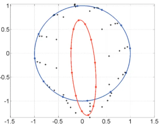
To illustrate the presented algorithm, we use it on a very small set of 12 planar data. Initially, they are all lying on a sharp ellipse (plotted in red in Figure 4). This scenario corresponds to strong scale factors, moderate bias, and misalignment. The algorithm is run over 4 iterations. Results are reported on top of each other in Figure 4. As can be observed, the data are quickly calibrated, i. e. they all get close to the unit circle within this small number of iterations.
Fig. 4. Evolution of the calibration over 4 iterations of the proposed algorithm. Measurements are in red and the unit circle in blue. The four iterations of the calibration algorithm are represented by black crosses.
C. A special case: 2 dimensional unbiased calibration prob-lem
The previously presented propositions provide theoretical insight into the progression of the algorithm along the itera-tions: the data are better and better calibrated (Proposition 1), and make few progress in rotation (Proposition 2). It is in fact possible to go a little bit further in the analysis. Let us now focus on a specific 2 dimensional case (i. e. where the measurements are done in 2D), and further, let us make the following simplifying assumptions. We consider that the measurements constitute a closed and centered ellipse (i.e. that there is a continuum of data, and that a preliminary debiasing has been performed). The measurements are noted 𝑦(𝜃), 𝜃 ∈ [0, 2𝜋[, and the iteratively calibrated data are 𝑦𝑘(𝜃),
𝜃 ∈ [0, 2𝜋[. Then, we assume that no misalignment is present and consider only scale factors. Therefore, the measurements satisfy
𝑌 (𝜃) = 𝐴𝑦(𝜃)
where 𝐴 is an unknown diagonal matrix. By analogy to
equation (4), the cost to be minimized at iteration𝑘 is ℎ(𝐴, 𝑘) = ∫ 2𝜋 0 2 2 2 2 𝐴𝑦𝑘(𝜃) − 𝑦𝑘(𝜃) ∥𝑦𝑘(𝜃)∥ 2 2 2 2 𝑑𝜃 Note𝐴𝑘+1 the solution of this minimization problem, i.e.
𝐴𝑘+1= arg min
𝐴 diagonalℎ(𝐴, 𝑘)
Iteratively, the data are calibrated using 𝑦𝑘+1(𝜃) =
𝐴𝑘+1𝑦𝑘(𝜃). At step 𝑘, let us note the inverse calibration
equation 𝑦𝑘(𝜃) = ( 𝛼𝑘 0 0 𝛽𝑘 ) 𝑌 (𝜃) With the notation
𝑓 (𝑦𝑘) = ∫ 2𝜋 0 ; ; ;1 − ∥𝑦𝑘(𝜃)∥ 2; ; ; 𝑑𝜃
a reasoning similar to the one in the proof of Proposition 2 directly yields 𝑓 (𝑦𝑘) ≥ ℎ(𝐴𝑘+1, 𝑘) ≥ 𝑓(𝑦𝑘+1) Further, 𝑓 (𝑦𝑘) = 2𝜋 ( 1 + 𝛼 2 𝑘 2 + 𝛽2 𝑘 2 ) − 2 ∫ 2𝜋 0 ∥𝑦(𝜃)∥ 𝑑𝜃 = 2𝜋 ( 1 + 𝛼 2 𝑘 2 + 𝛽2 𝑘 2 ) − 2𝑃 (𝛼, 𝛽) (14)
where 𝑃 (𝛼, 𝛽) is the perimeter of an ellipse having 1/𝛼𝑘
and 1/𝛽𝑘 as semi-axis. We wish to show that the inverse
calibration matrix (
𝛼𝑘 0
0 𝛽𝑘
)
tends to the identity as k tends to infinity, i.e. that the proposed algorithm converges to exact calibration of the data. Similarly to Proposition 1,
one can readily show that 𝑓 decreases along the iterations
and goes to a limit ℓ ≥ 0. Using an estimate for (14), it is possible to deduce convergence information on𝛼𝑘 and𝛽𝑘.
To simplify the exposition, let us first consider that this limit isℓ = 0.
Consider in equation (14),𝑓 as a function of (𝛼𝑘, 𝛽𝑘). It
can be proved that𝑓 has (1, 1) as unique local minimum (in a rather large neighborhood) and that its value there is0. To prove that, one can simply use Peano’s approximation of the perimeter of an ellipse [1] reproduced in (17). Accounting for the approximation implied by this formula, one can compute
the following exact decomposition of𝑓 under the form
𝑓 (𝛼𝑘, 𝛽𝑘) = 𝑓1(𝛼𝑘, 𝛽𝑘) + 𝑓2(𝛼𝑘, 𝛽𝑘)
where 𝑓2(𝛼𝑘, 𝛽𝑘) is strictly positive away from 𝛼𝑘 = 𝛽𝑘
and zero there, while 𝑓1, given in (18), is convex on the
considered domain[3/4 4/3]2
(its Hessian is given in (19)), strictly positive away from(1, 1) and zero there. Therefore, (1, 1) is the only zeroing point of 𝑓 , and one can conclude that(𝛼𝑘, 𝛽𝑘) converges to (1, 1). This estimate reveals handy
in experimental results whereℓ can be evaluated numerically. Now, let us extend the analysis to the caseℓ > 0. A local expansion of𝑓 for (𝛼, 𝛽) about (1, 1) yields the following inequalities ( 𝛼 − 1 𝛽 − 1 ) ⎛ ⎝ 3 1 1 3 ⎞ ⎠ ⎛ ⎝ 𝛼 − 1 𝛽 − 1 ⎞ ⎠ 16 ≤ ℓ ℓ ≤ ( 𝛼 − 1 𝛽 − 1 ) ⎛ ⎝ 3 1 1 3 ⎞ ⎠ ⎛ ⎝ 𝛼 − 1 𝛽 − 1 ⎞ ⎠ 4
and we deduce the estimation, where 𝑑 is the distance of
(𝛼, 𝛽) to (1, 1), √ 2 4 𝑑 ≤ √ ℓ ≤ 𝑑 (15)
meaning that both𝛼𝑘 and𝛽𝑘 approach1 as the square root
ofℓ approaches 0.
!"#$%&'
2 4 6 8 10 12 14 16 -1.08 -1.06 -1.04 -1.02 -1 -0.98 -0.96 -0.94 -0.92 Iterations log(S)
Log of the standard error S
Iterative algorithm 2-step algorithm
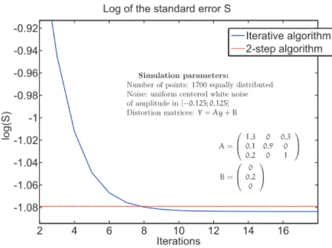
Simulation parameters: Number of points: 1700 equally distributed Noise: uniform centered white noise of amplitude in [−0.125; 0.125] Distortion matrices:Y = Ay + B A = ⎛ ⎝ 1.3 0 0.3 0.1 0.9 0 0.2 0 1 ⎞ ⎠ B = ⎛ ⎝ 0 0.2 0 ⎞ ⎠
Fig. 6. Evolution of the standard error S over a few iterations of the iterative algorithm proposed and comparison with the results obtained with the 2-step algorithm
IV. EXPERIMENTAL RESULTS
Several experiments have been conducted using the hard-ware presented in Section I-C. To evaluate the performance of the algorithms, the standard error S is used.
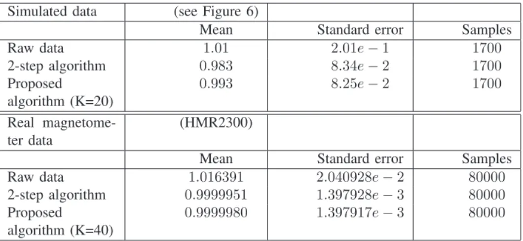
𝑆(𝑦) = 1 𝑁 − 1⋅ 𝑁 ∑ 𝑖=1 (∥𝑦𝑖∥ − 1) 2 (16) Table 5 shows some results obtained with simulated data and with less disturbed real data from a magnetometer (HMR2300 from HoneywellⓇ). It appears that the calibra-tion process allows significant improvement compared to the raw data. The standard error S used to evaluate the various algorithms is better for the proposed iterative one. When cross-coupling terms are small, on the one hand, improvement brought by this algorithm get smaller, but, on the other hand, fewer iterations are needed and computation time is faster.
To underline the possibly erratic behavior of the 2-step algorithm in extreme cases (see Section II-A ), we consider a set of 1700 perfectly scaled unbiased 3D data, and introduce a strong misalignment which is varied from 0 to 40. As can be seen in Figure 7, when the misalignment term (one of the upper triangular part of matrix A) reaches the values of 20 (approximately), the 2-step algorithm ends up with ill-calibrated data. Both the standard error and the mean value are inconsistent with reality. Interestingly, the proposed algorithm keeps working properly.
Finally, accuracy of the proposed method can be investi-gated. By increasing the number of iterations, the accuracy is enhanced. This point is visible in Figure 6. In this plot, the log of the standard error is plotted for various numbers of iterations, giving an idea of the rate of convergence. It appears in the considered scenario (1700 simulated data with matrix and bias reported in the figure), that the proposed algorithm outperforms the 2-step method as soon as the number of iterations is larger than 10.
0 10 20 30 40 -15 -10 -5 0 Standard error S Log( S ) 0 10 20 30 40 0 5 10 15
Mean Interative algorithm 2-step algorithm
Fig. 7. Erratic behavior. A set of 1700 perfectly scaled unbiased 3D data is considered, and a strong misalignment which is varies from 0 to 40 is introduced. Mean and standard error S are given for both the 2-step algorithm (in red) and the proposed one (in blue).
V. CONCLUSION
In this paper, we have introduced a new algorithm for calibrating three-axis sensors. This iterative method makes a repeating use of least-squares algorithm. As has been demonstrated, it proves very effective when treating large sets of uncalibrated data. Certainly, the numerical efficiency of the method can be improved upon, by reusing key information from one iteration to the next for example. We also believe that more theoretical results can be obtained. Several points remains to be explored, in particular the magnitude of the residual error seems to be possible to estimate. Finally, an extension of the proposed algorithm is currently considered. It aims at calibrating at once an array of sensors by including corrections of the misalignment between the sensorsmeasuring the same force field. These are current directions of future work.
REFERENCES
[1] R. W. Barnard, K. Pearce, and L. Schovanec. Inequalities for the perimeter of an ellipse. Journal of Mathematical Analysis and Applications, 260(2):295 – 306, 2001.
[2] C. Barton. Revision of International Geomagnetic Reference Field Release. EOS Transactions, 77, April 1996.
[3] P. Castillo, A. Dzul, and R. Lozano. Real-time stabilization and tracking of a four rotor mini rotorcraft. IEEE Trans. Control Systems Technology, 12(4):510–516, 2004.
[4] S. Changey, D. Beauvois, and V. Fleck. A mixed extended-unscented filter for attitude estimation with magnetometer sensor. In Proc. of the 2006 American Control Conference, 2006.
[5] A. B. Chatfield. Fundamentals of High Accuracy Inertial Navigation, volume 174 of Progress in Astronautics and Aeronautics Series. AIAA, 1997.
[6] E. Dorveaux, D. Vissière, A. P. Martin, and N. Petit. Time-stamping for an array of low-cost sensors. In Proc. of the PDES 2009, IFAC workshop on Programmable Devices and Embedded Systems, 2009. [7] P. Faurre. Navigation inertielle et filtrage stochastique. Méthodes
mathématiques de l’informatique. Dunod, 1971.
[8] W. T. Fong, S. K. Ong, and A. Y. C. Nee. Methods for in-field user calibration of an inertial measurement unit without external equipment. Measurement Science and Technology, 19(8):085202–+, Aug. 2008. (EB6
Simulated data (see Figure 6)
Mean Standard error Samples
Raw data 1.01 2.01𝑒 − 1 1700 2-step algorithm 0.983 8.34𝑒 − 2 1700 Proposed algorithm (K=20) 0.993 8.25𝑒 − 2 1700 Real magnetome-ter data (HMR2300)
Mean Standard error Samples
Raw data 1.016391 2.040928𝑒 − 2 80000
2-step algorithm 0.9999951 1.397928𝑒 − 3 80000
Proposed
algorithm (K=40)
0.9999980 1.397917𝑒 − 3 80000
Fig. 5. Numerical calibration results for a set of simulated data and a set of experimental measurements.
[9] C. Foster and G. Elkaim. Extension of a non-linear, two-step calibration methodology to include non-orthogonal sensor axes. In IEEE Journal of Aerospace Electronic Systems, volume 44, July 2008. [10] D. Gebre-Egziabher, G. Elkaim, J. Powell, and B. Parkinson. A non-linear, two-step estimation algorithm for calibrating solid-state strap-down magnetometers. In 8th International St. Petersburg Conference on Navigation Systems (IEEE/AIAA), May 2001.
[11] M. S. Grewal, L. R. Weill, and A. P. Andrews. Global positioning systems, inertial navigation, and integration. Wiley Inter-science, 2001.
[12] R. Mahony, T. Hamel, and J.-M. Pflimlin. Complementary filter design on the special orthogonal group SO(3). In Proc. of the 44th IEEE Conf. on Decision and Control, and the European Control Conference 2005, 2005.
[13] P. Ripka, editor. Magnetic Sensors and Magnetometers. ed. Boston: ARTECH HOUSE, 1. edition, 2001.
[14] I. Skog and P. Händel. Calibration of a mems inertial measurement unit. In XVII IMEKO World Congress Metrology for a Sustainable Development, Sept. 2006.
[15] D. Vissière, P.-J. Bristeau, A. P. Martin, and N. Petit. Experimental au-tonomous flight of a small-scaled helicopter using accurate dynamics model and low-cost sensors. 2008.
[16] D. Vissière, A. P. Martin, and N. Petit. Using magnetic disturbances to improve IMU-based position estimation. In Proc. of the 9th European Control Conf., 2007.
APPENDIX
Peano’s approximation of the perimeter of the ellipse is always over-estimating the true value. Here is the approxi-mation: 𝑃 (𝛼, 𝛽) ≈ 𝜋( 32(𝛼 + 𝛽) −√𝛼𝛽 ) (17) which yields to 𝑓1(𝛼, 𝛽) = 2𝜋 ( 1 +𝛼 2 2 + 𝛽2 2 ) − 2𝜋( 32(𝛼 + 𝛽) −√𝛼𝛽 ) (18) The hessian of𝑓1 is the following one
∇2𝑓 1(𝛼, 𝛽) 2𝜋 = ( 1 −4𝛼√𝛽𝛼𝛽 1 4√𝛼𝛽 1 4√𝛼𝛽 1 − 𝛼 4𝛽√𝛼𝛽 ) (19) !"#$%&' (EBE