HAL Id: hal-01791317
https://hal.archives-ouvertes.fr/hal-01791317
Submitted on 14 May 2018
HAL is a multi-disciplinary open access
archive for the deposit and dissemination of
sci-entific research documents, whether they are
pub-lished or not. The documents may come from
teaching and research institutions in France or
abroad, or from public or private research centers.
L’archive ouverte pluridisciplinaire HAL, est
destinée au dépôt et à la diffusion de documents
scientifiques de niveau recherche, publiés ou non,
émanant des établissements d’enseignement et de
recherche français ou étrangers, des laboratoires
publics ou privés.
Kinematic analysis of planar tensegrity 2-X
manipulators
Matthieu Furet, Max Lettl, Philippe Wenger
To cite this version:
Matthieu Furet, Max Lettl, Philippe Wenger. Kinematic analysis of planar tensegrity 2-X
manipu-lators. 16th International Symposium on Advances in Robot Kinematics, Jul 2018, Bologne, Italy.
�hal-01791317�
manipulators
Matthieu Furet1,2, Max Lettl1, and Philippe Wenger1,2
1
Ecole centrale de Nantes, 44321 Nantes, France
2
Laboratoire des Sciences du Numérique de Nantes (LS2N), CNRS, 44321 Nantes, France
Abstract. This paper analyzes the kinematics of planar tensegrity ma-nipulators made of two Snelson’s X-shape mechanisms in series. The variable instantaneous center of rotation of each mechanism renders the kinematic analysis of the resulting manipulator more challenging. A gen-eral formulation of the direct kinematics is set. A method is proposed to solve the inverse kinematic problem in a symbolic way and up to four in-verse kinematic solutions are found. The singularities of the manipulator are shown to divide the joint space into two singularity-free components, showing for the first time a planar positioning manipulator that can be cuspidal. The workspace is determined and plotted for different values of the geometric parameters.
Keywords: Tensegrity, Kinematics, Singularity, Workspace, Cuspidal
1
Introduction
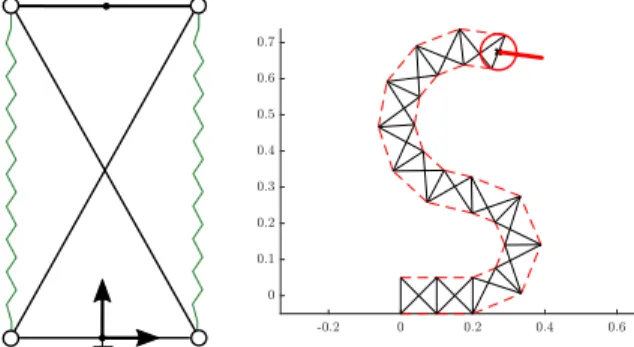
A tensegrity structure is an assembly of compressive elements (bars) and tensile elements (cables, springs) held together in equilibrium [1],[3]. Tensegrity is known in architecture and art for more than a century [2] and is suitable for modeling living organisms [4]. Tensegrity mechanisms have been more recently studied for their promising properties in robotics such as low inertia, natural compliance and deployability [5],[6],[7]. A tensegrity mechanism is obtained when one or several elements are actuated. This work falls withing the context of the AVINECK project involving biologists and roboticists with the main objective to model and design bird necks. Accordingly, a class of planar tensegrity manipulators made of a series assembly of several Snelson’s X-shape mechanisms [8] i.e. crossed four-bar mechanisms with springs along their lateral sides, has been chosen as a suitable candidate for a preliminary planar model of a bird neck, see figure1. First investigations on the kinematics of such manipulators turn out to be more challenging than expected with interesting properties, which has motivated the work presented in this paper. Snelson’s X-shape mechanisms have been studied by a number of researchers, either as a single mechanism [5],[7],[9] or assembled in series [10],[11],[12]. A planar two-degree-of-freedom manipulator is obtained with a series assembly of two such mechanisms. The manipulator can be driven with tendons threaded through the spring attachment points like in [12], or
2 Matthieu Furet et al.
it can be actuated with a rotary motor at a base joint of each mechanism. There are several possible actuation schemes that can involve over-actuation if stiffness needs also to be controlled [10]. The detailed actuation scheme is not reported here and will be the scope of further work. This paper focuses on the full kinematic analysis of the manipulator, which has never been done before to the best of the authors’ knowledge. The variable instantaneous center of rotation of each mechanism renders the symbolic calculation of the inverse geometric problem more challenging, resulting in polynomials of excessive degree if the problem is not tackled with care. A practical method is provided that makes it possible to come up with a quartic polynomial, which turns out to be of minimal degree. The singularities of the manipulator are shown to divide the joint space into two singularity-free components or aspects, showing for the first time a planar positioning manipulator that is cuspidal i.e. that can perform non-singular solution changing motions. The workspace is calculated with its boundaries for different values of the geometric parameters.
Fig. 1: Snelson’s X-shape mechanism (left) and a series assembly of several such mechanisms, mimicking a bird neck (right)
2
Derivation of the kinematic equations
2.1 Manipulator description and parametrization
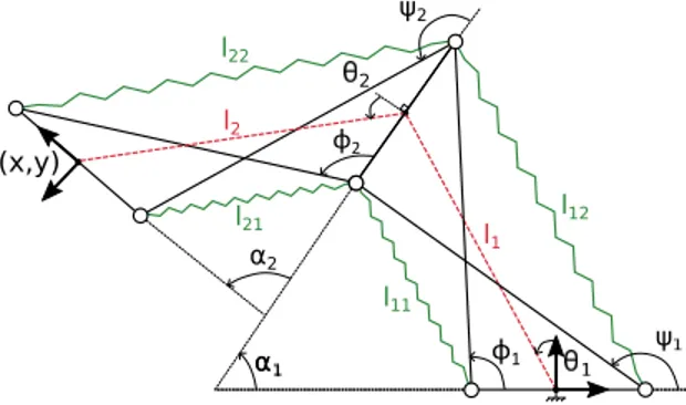
The manipulator studied consists of a series assembly of two identical crossed-bar mechanisms as shown in figure2. Each mechanism i has a base bar and an upper bar of length b and two crossed bars of length L. Note that the mechanism assembly condition is L>b. The springs, shown in green in figures1and2, are of length lij. We need to define a suitable joint variable that describes each mecha-nism configuration without any ambiguity. In [12], the mechanism configuration was chosen as the orientation αi of the upper bar with respect to the base bar, but such a choice is allowed for mechanism motions restricted to −π < αi < π. For a matter of completeness, we are interested in allowing each mechanism to
move within its full range. In this case,−2π < αi < 2π and αi is not appropriate to define the mechanism configuration. Let us introduce a line segment of length li that links the middle points of the top and base bars of each mechanism i (shown in red dotted line in figure 2). The angle between this line and the di-rection orthogonal to the base bar is referred to as θi. For the symmetric design considered here, it can be shown that αi = 2θi and when −π < θi < π, the mechanism makes a full turn. Assuming that each mechanism remains always in the crossed-bar assembly mode, the manipulator configuration can thus be fully defined with (θ1, θ2). Since the mechanism sides define an isosceles trapezoid,
α α α2 2 ψ ψ2 l1 l2 l11 l12 l21 l22 (x,y) φ2 φ1
Fig. 2: Manipulator description
the length liof the line segment that links the middle points of the top and base bars can be expressed as follows :
li(θi) = li1+ li2 2 =
p
L2− b2cos2(θi) (1)
2.2 Direct Kinematics
We first want to establish the direct kinematic equations. The base frame is centered at the middle point of the base bar with the x-axis aligned along this bar. The reference point (x, y) is chosen as the middle point of the top-bar (figure 2). Note that any other location on the top bar would not affect the study, with the exception of one of the two extremities. In such a case, indeed, the input/output equations would be the same as in a simple 2R planar manipulator and the kinematic properties of the manipulator studied would not be captured. The direct kinematic equations of a manipulator with n mechanisms in series can be written as for a virtual serial nR manipulator with (varying) link lengths li and joint angles θi:
(
x =Pni=1li(θi) cos(π−2θi
2 + Pi
j=12θj) y =Pni=1li(θi) sin(π−2θi
2 + Pi
j=12θj)
4 Matthieu Furet et al.
For a manipulator made of two mechanisms in series with input variables θ1and θ2, the direct kinematic equations can be put in the following form :
(
x = −l1(θ1) sin(θ1) − l2(θ2) sin(2θ1+ θ2)
y = l1(θ1) cos(θ1) + l2(θ2) cos(2θ1+ θ2) (3) where l1 and l2 are defined in (1). Note that these equations assume that each mechanism is in its crossed-bar assembly-mode.
2.3 Inverse Kinematics
We would like now to derive the so-called characteristic polynomial, a univariate polynomial established to solve the inverse kinematics. The direct kinematic equations (3) have been derived in their most compact form, namely, the two output variables x and y are expressed as a function of the two input variables θ1and θ2like in a 2R serial manipulator. However, starting from these equations to derive a characteristic polynomial is not appropriate. Indeed, the square roots appearing in l1and l2should be first cleared out, with the consequence of raising artificially the degree of the resulting characteristic polynomial and providing spurious solutions. Accordingly, it is better to write x and y as functions of the crossed-bar angles φ1 and ψ2as follows:
( x = −b
2+ L cos(φ1) + L cos(ψ2+ α1) + 1
2b cos(α1+ α2)
y = L sin(φ1) + L sin(ψ2+ α1) +12b sin(α1+ α2) (4) In addition, the two loop-closure equations below are derived:
(
−2Lb sin(α1) sin(φ1) − 2Lb(cos(α1) + 1) cos(φ1) + 2b2(cos(α1) + 1) = 0 2Lb sin(α2) sin(ψ2) + 2Lb(cos(α2) + 1) cos(ψ2) + 2b2(cos(α2) + 1) = 0
(5) A set of four equations in four unknowns is thus available. A univariate polyno-mial can be obtained upon elimination of three of the four unknowns. There are several ways to do so with a computer algebra software. We have used Maple and its Siropa library [14]. This library was developed in the frame of a collab-orative project on the kinematics of parallel manipulators, see e.g. [15], [16] for more details on the implementation and use of these tools. It contains specific macro-functions that use efficient algebraic tools such as Groebner bases. Specif-ically, the Projection function was used to project the system of four equations in order to obtain one single equation in one single variable, chosen here as φ1. The half-tangent substitution yields a factored polynomial, one of which defines the characteristic polynomial. The characteristic polynomial obtained turns out to be of degree 4 in t=tan(φ1/2) and can be written as follows:
a4t4+ a3t3+ a2t2+ a1t + a0= 0 (6) where :
a3= 4y(b + 1)(2b2x + b2− 2x2− 2y2− 4x − 1) (8) a2= 2(b4y2+ b2x4+ 2b2x2y2+ b2y4+ b2x2− 10b2y2+ x4+ 2x2y2+ y4− 3x2+ 9y2) (9) a1= 4y(b − 1)(2b2x − b2+ 2x2+ 2y2− 4x + 1) (10) a0= (b − 1)2(b2y2+ x4+ 2x2y2+ y4− 4x3− 4xy2+ 5x2+ y2− 2x) (11) Note that L was set equal to 1 to simplify the calculations without loss of generality. For each solution φ1, α1 is then solved from the first equation in (5) (disregarding the solution α1= π corresponding to the parallelogram assembly):
tan(α1/2) = −L cos(φ1) + b
L sin(φ1) (12)
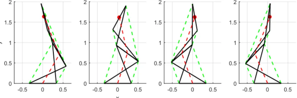
Finally, ψ2 and α2 are solved from system (4), which gives two solutions, one of which never satisfies the closed-loop equations (5). In total, thus, one comes up with a maximum number of four solutions. The inverse kinematics is solved for a manipulator defined by L = 1 and b = 2/3 at x = 0.03 and y = 1.6. Four solutions are found (see figure3), showing that the characteristic polynomial (6) is of minimal degree. -0.5 0 0.5 0 0.5 1 1.5 2 y -0.5 0 0.5 x 0 0.5 1 1.5 2 -0.5 0 0.5 0 0.5 1 1.5 2 -0.5 0 0.5 0 0.5 1 1.5 2
Fig. 3: The four inverse solutions at x = 0.03 and y = 1.6 (L = 1 and b = 2/3)
3
Singularity analysis and aspects
The Jacobian matrix of the manipulator is derived from system (3) and its determinant is calculated and can be put in the following form:
Det(J ) = (sin(θ1)2b2cos(θ1) − (L2− b2cos(θ1)2)(cos(θ1) + 2 cos(θ2+ 2θ1))) (cos(θ2+ 2θ1)b2cos(θ2) sin(θ2) − (L2− b2cos(θ2)2) sin(θ2+ 2θ1)) −(− sin(θ2+ 2θ1)b2cos(θ2) sin(θ2) − (L2− b2cos(θ2)2) cos(θ2+ 2θ1)) (cos(θ1)2b2sin(θ1) − (L2− b2cos(θ1)2)(sin(θ1) + 2 sin(θ2+ 2θ1)))
6 Matthieu Furet et al.
Solving Det(J ) = 0 for θ1yields two solution sets. The first one is θ1= −θ2± π and means that the two modules are coincident. It is equivalent to the fully-folded back configuration of a planar 2R serial manipulator. When the manipulator is in this singularity, the reference point is at the origin x = 0 and y = 0, whatever θ1. The second solution is given by:
θ1= atan2(− sin(θ2)(4b4cos(θ2)4− 4L2b2cos(θ2)2− L2b2+ L4), cos(θ2)(4b4cos(θ2)4− 4b4cos(θ2)2− 4L2b2cos(θ2)2+ 3L2b2+ L4)) (14) This solution is associated with the configuration where the two instantaneous centers of rotation (ICR) are aligned with the end-effector control point, like in the fully outstretched configuration of a planar 2R serial manipulator. In this singularity, the manipulator cannot produce an instantaneous motion along a line passing through the two mechanism ICR and the end-effector control point. The above singularities divide the joint space into singularity-free domains called
- - /2 0 /2 1 -- /2 0 /2 2
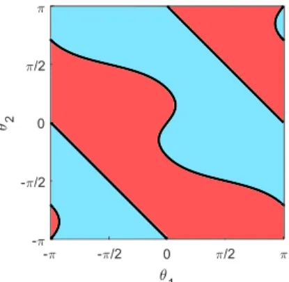
Fig. 4: Singularity curves in the joint space and aspects when L = 1 and b = 2/3
aspects [17]. The singularity θ1= −θ2±π produces two lines while the singularity defined by equation (14) gives a curve, as shown in figure4. In the absence of joint limits, the opposite sides of the square are in fact coincident and the singularity curves divide the joint space into only two aspects. Since the manipulator admits up to four solutions, there are two solutions in each aspect, which means that the manipulators can move from one inverse kinematic solution to another without meeting a singularity, namely, it is cuspidal [19]. To the authors’ knowledge, it is the first time that a planar positioning manipulator is shown to be cuspidal.
4
Workspace analysis
When plotted into the workspace, the singularity curves define its boundaries. The equation of these curves can be obtained by deriving the discriminant of
the characteristic polynomial (6). By doing so, a polynomial of degree 16 in x and y is obtained. Its expression is quite large and shall not be reported here for lack of space. Figure5 shows the plot of these curves for three examples. In the second and third figures, they divide the workspace into three regions. In the largest one, the manipulator admits two inverse kinematic solutions. In the two smaller regions, there are four solutions. Clearly, the 4-solution regions get larger when b is increased. The boundaries of these two 4-solution regions have three singular points: a node and two cusps. The existence of cusps confirms the fact that the manipulator is cuspidal. A non-singular solution changing motion can be defined by encircling one of the cusps [18], [19]. Note that the two aspects map onto the whole workspace, namely, figure5 also shows the image of any of the two aspects.
-2 -1 0 1 2 x -2 -1 0 1 2 y -2 -1 0 1 2 x -2 -1 0 1 2 y -2 -1 0 1 2 x -2 -1 0 1 2 y
Fig. 5: Workspace boundaries when L = 1 and b = 2/5 (left), b = 2/3 (center), b = 9/10 (right)
5
Conclusion
The complete kinematic analysis of a planar manipulator made of two X-four bar mechanisms in series has been carried out. The manipulator was shown to have two or four solutions depending on its geometric parameter values. When it has four solutions, the manipulator turns out to be cuspidal, a result that was not expected. The influence of the geometric parameters on the shape and size of the workspace was analyzed. The influence of joint limits was not reported for lack of space and shall be studied in a near future as they also play an important role. Internal collisions were not considered since a suitable design by assembling the rods in different planes allows avoiding any physical interference. Future work will be conducted on the actuation strategy.
Acknowledgement This work was conducted with the support of the French National Research Agency (AVINECK Project ANR-16-CE33-0025).
8 Matthieu Furet et al.
References
1. R. B. Fuller, Tensile-integrity structures, United States Patent 3063521,1962 2. Skelton, R. and de Oliveira, M., Tensegrity Systems. Springer, 2009
3. Motro, R. Tensegrity systems: the state of the art, Int. J. of Space Structures, 7 (2), pp 75–83, 1992
4. S. Levin, The tensegrity-truss as a model for spinal mechanics: biotensegrity, J. of Mechanics in Medicine and Biology, Vol. 2(3), 2002
5. M. Arsenault and C. M. Gosselin, Kinematic, static and dynamic analysis of a planar 2-dof tensegrity mechanism, Mech. and Mach. Theory, Vol. 41(9), 1072-1089, 2006 6. C. Crane et al., Kinematic analysis of a planar tensegrity mechanism with
pres-stressed springs, in Advances in Robot Kinematics: analysis and design, pp 419-427, J. Lenarcic and P. Wenger (Eds), Springer (2008)
7. P. Wenger and D. Chablat, Kinetostatic Analysis and Solution Classification of a Planar Tensegrity Mechanism, proc. 7th. Int. Workshop on Comp. Kinematics, Springer, ISBN 978-3-319-60867-9, pp422-431, 2017.
8. K. Snelson, 1965, Continuous Tension, Discontinuous Compression Structures, US Patent No. 3,169,611
9. Q. Boehler et al., Definition and computation of tensegrity mechanism workspace, ASME J. of Mechanisms and Robotics, Vol 7(4), 2015
10. JB Aldrich and RE Skelton, Tienergy optimal control of hyper-actuated me-chanical systems with geometric path constraints, in 44th IEEE Conference on De-cision and Control, pp 8246-8253, 2005
11. S. Chen and M. Arsenault, Analytical Computation of the Actuator and Cartesian Workspace Boundaries for a Planar 2-Degree-of-Freedom Translational Tensegrity Mechanism, Journal of Mech. and Rob., Vol. 4, 2012
12. D. L Bakker et al., Design of an environmentally interactive continuum manipula-tor, Proc.14th World Congress in Mechanism and Machine Science, IFToMM’2015, Taipei, Taiwan, 2015
13. M. Lettl., Kinetostatic analysis of tensegrity mechanisms, application to the mod-elling of bird necks, Master thesis, Ecole Centrale de Nantes, France, 2017
14. F. Rouillier et al., Siropa Library V1, IDDN.FR.001.140015.000.S.P.2017.000.20600. 15. M. Manubens et al., Cusp Points in the Parameter Space of Degenerate 3-RPR
Planar Parallel Manipulators, ASME J. of Mechanisms and Robotics, Vol. 4(4), 2012
16. G. Moroz et al., On the determination of cusp points of 3-RPR parallel manipula-tors, Mechanism and Machine Theory 45 (11), pp. 1555-1567, 2011
17. P. Borrel and A. Liegeois, A study of manipulator inverse geometric solutions with application to trajectory planning and workspace determination.
18. J. El Omri and P. Wenger, How to recognize simply a non-singular posture changing manipulator, Proc. 7th Int. Conf. on Advanced Robotics, 215-222, 1995
19. P. Wenger, Cuspidal and noncuspidal robot manipulators. Special issue of Robotica on Geometry in Robotics and Sensing, Volume 25(6), pp.677-690, 2007