Unsupervised segmentation of sequences using harmony search and hierarchical clustering techniques

(1)

Unsupervised segmentation of sequences using Harmony

Search and hierarchical clustering techniques

Mémoire

Asra Roshani

Maîtrise en informatique

Maître ès sciences (M.Sc.)

Québec, Canada

© Asra Roshani, 2014

(2)

(3)

III

Résumé

Dans le contexte de traitement automatique du langage naturel, les données le plus souvent sont présentées comme une longue séquence de caractères discrets. Donc, l'identification d'un modèle intéressant dans la longue séquence peut être une tâche difficile. En conséquence, la segmentation automatique de données serait extrêmement utile pour extraire les sous-séquences et les morceaux significatifs à partir d'une longue séquence de données. La segmentation de données est l'une des étapes de prétraitement les plus importantes dans plusieurs tâches de traitement du langage naturel. La segmentation de mots est considérée comme la tâche de trouver des morceaux significatifs dans le corpus de textes. L'objectif principal de cette étude est de présenter une technique de segmentation hiérarchique non supervisée en utilisant l'algorithme de recherche d'harmonie (Harmony

Search algorithm) qui est une approche d'optimisation méta-heuristique. Dans la technique

proposée, la tâche de segmentation de mots est réalisée à l'aide d'une recherche d'harmonie binaire (Binary Harmony search) qui une forme particulière de l'algorithme de recherche d'harmonie. La construction et la formation de modèles de langue sont accomplies par un lexique hiérarchique et un algorithme de Baum-Welch. De plus, pour améliorer la performance et la convergence de la recherche de l'harmonie binaire, quelques modifications innovantes sont appliquées. En général, cette étude présente un algorithme de segmentation de mots hiérarchique non supervisée basée sur une méthode recherche de l'harmonie et examine toutes les questions relatives y compris: la segmentation de mots représentées en format binaire, l'harmonie binaire, l'amélioration de la procédure de l'ajustement du lancement, la définition de la fonction objective en recherche d'harmonie et la politique de pénalité. La performance de l'algorithme est évaluée selon la précision de la segmentation, le rappel, la F-mesure et le temps d'exécution de l'algorithme. Une partie du corpus Moby Dick est utilisée comme étude de cas. Nos expérimentations montrent que l'approche de segmentation basée sur une recherche d'harmonie fournit plusieurs de bons segments, mais qu'il nécessite un long temps d'exécution.

(4)

(5)

V

Abstract

In the context of natural language processing, data is presented most of the time as a long sequence of discrete characters. Therefore, identifying interesting patterns within the long sequence can be a challenging task. Consequently, automatic segmentation of data would be extremely useful to extract the meaningful sub-sequences and chunks from a long data sequence. Segmentation of raw data is one of the most important preprocessing steps in many natural language processing tasks. Word segmentation is considered as the task of finding meaningful chunks, i.e. words, within a text corpus. The main objective of this study is to present an unsupervised hierarchical segmentation technique using Harmony Search algorithm which is a meta-heuristic optimization approach. In the proposed technique, the word segmentation task is performed using a Binary Harmony Search (a special form of Harmony Search). The language model construction and training are accomplished using a hierarchical lexicon and Baum-welch algorithm. Moreover, to improve the performance and convergence of the Binary Harmony Search, some innovative modifications are applied. In general, this study introduces an unsupervised hierarchical word segmentation algorithm based on Harmony Search approach and investigates the following related issues: word segmentation mapping to binary format, Binary Harmony Search, pitch adjustment procedure improvement, Harmony Search objective function definition, and penalty policy. The performance of the algorithm is valuated using segmentation precision, recall, F-measure and the algorithm run time when applied to the part of famous Moby Dick story as the case study. Our experiments reveal that the segmentation approach based on Harmony Search provides significantly good segments, while it requires significant run time.

(6)

(7)

VII

List of Tables

Table 2-1: Decoding a gene in Binary genetic algorithm ... 29

Table 5-1: Properties of our experiment dataset (Moby Dick) ... 60

Table 5-2: Mutual Information at different levels of the hierarchical lexicon for Moby Dick. ... 62

Table 5-3: Corpus size effect on UHS performance. ... 66

Table 5-4: Effect of various MI parameters tuning scenarios on the UHS performance (5-chapter). ... 67

Table 5-5: HS tuning parameters for the optimum point. ... 72

(10)

(11)

XI

List of Figures

Figure 2-1: Algorithm of K-Means Data Clustering ... 6

Figure 2-2: The dendrogram of the hierarchical clustering method. ... 7

Figure 2-3: The probability of traversing an arc from state i to j: the α and β probabilities, the transition probability aijand the observation probability b oj( t+1) [Jurafsky and Martin, 2000]. ... 14

Figure 2-4: Example sequences and grammars that reproduce them: (a) a sequence with one repetition; (b) a sequence with a nested repetition; (c) two grammars that violate the two constraints; (d) two different grammars for the same sequence that obey the constraints [Nevill-Manning and Witten, 1997a]. ... 19

Figure 2-5: The six main categories of optimization algorithms [Haupt and Haupt, 2004]. ... 21

Figure 2-6: One-point crossover ... 25

Figure 2-7: Two-point crossover ... 25

Figure 2-8: Uniform crossover ... 26

Figure 2-9: Genetic Algorithm flowchart ... 28

Figure 2-10: Binary genetic algorithm... 30

Figure 2-11: General procedure of a continuous genetic algorithm ... 31

Figure 3-1: Example to illustrate the segmentation notation. ... 34

Figure 3-2: General flowchart of UHS using Viterbi ... 35

Figure 3-3: The cycle of interaction in UHS ... 36

Figure 3-4: Algorithm for unsupervised hierarchical segmentation [Shani et al., 2009]. ... 36

Figure 3-5: Build hierarchical lexicon based on segments ... 38

Figure 3-6: Baum-Welch algorithm. ... 41

Figure 3-7: The boundary of a word in a sequence. ... 44

Figure 4-1: General flowchart of UHS using Harmony Search ... 46

Figure 4-2: General procedure of the Harmony Search algorithm. ... 51

Figure 4-3: Fixed size window over the sequence of letters ... 52

Figure 4-4: Conversion of a letter sequence to binary vector and vice versa. ... 53

Figure 4-5: Segmentation for a given text window ... 54

Figure 5-1: An extract of the Moby Dick dataset ... 60

Figure 5-2: An extract of the preprocessed Moby Dick dataset ... 61

Figure 5-3: Baum-welch convergence for “is” segment during one UHS iteration. ... 63

Figure 5-4: Baum-welch convergence for “is” segment during multiple UHS iterations. ... 64

Figure 5-5: Performance of the Viterbi based UHS algorithm (blue line with ▪ marker: recall-precision, and green line with • marker: F-measure-precision). ... 68

Figure 5-6: Sample of text segmentation using Viterbi based UHS. ... 69

Figure 5-7: HS fitness function convergence. ... 71

Figure 5-8: Performance of the Harmony Search based UHS algorithm (blue line with ▪ marker: recall-precision, and green line with • marker: F-measure-precision). ... 72

Figure 5-9: Sample of text segmentation using HS based UHS. ... 73

(12)

(13)

XIII

Acknowledgment

First, I would like to express the deepest appreciation to my supervisor, Prof. Luc Lamontage for accepting me as a Master student, for all time and effort he has invested in my project and for his patience, helpful advices during this research work. I learned a lot from him in this thesis.

Besides my supervisor, I would like to thank my dear and loving husband, Amir for his never ending supports and helpful advices in my project.

I am also very thankful to my lab mates and my great friends in Canada especially Mona, Hamid, Leila, Mona, Alireza, Amir, Saghar and Neda for their academic advices and personal supports.

Finally and most important, I am grateful to my brothers, Omid and Amin, and my parents who have trusted and encouraged me in my life. This study would not have been possible without their support and love. To them I dedicate this thesis.

(14)

(15)

1

Chapter 1. Introduction

Because of language essential role in human beings’ life, they have always tried to systematically process and model it. In general, it is a challenging task due to language complexity and vagueness. It can even be more difficult when machines attempt to understand and model language. Language ambiguities are even hard to be understood by human, and obviously machines have more difficulties. But grandeur and complexity of the language models makes unavoidable the use of machines. Based on this need, Natural Language Processing (NLP) has been introduced as a field of Artificial Intelligence (AI) and linguistics. NLP attempts to facilitate the interactions between computers and human languages. At present, computers are not fully able to understand our ordinary language and meanings, and it is the greatest barrier separating us from machines. The goal of research in NLP is to break down this barrier.

The history of NLP generally started in the 1950s when Alan Turing (Turing, 1950) published an article entitled "Computing Machinery and Intelligence". This paper proposed

Turing test known as a criterion of intelligence. Since then a lot of researches have been

accomplished in NLP context. During the 1960s, some successful NLP systems developed such as SHRDLU (a natural language system working in “blocks worlds” with restricted vocabularies) and ELIZA (a simulation of a Rogerian psychotherapist). During the 1970s, many algorithms were developed by programmers to convert real-world information into computer-understandable data. Examples are MARGIE [Schank, 1975], QUALM [Lehnert, 1977], Politics [Carbonell, 1979] and PAM [Wilensky et. al, 1980]. Up to the 1980s, most NLP systems were based on complex sets of hand-written rules. In late 1980s, a revolution in NLP was occurred with the introduction of machine learning algorithms for language processing. This was because of the increase in computational power resulting from Moore’s Law, and the lessening of Chomskyan theories of linguistics [Chomsky, 1957]. Instead of hand-written models, research has mainly focused on statistical models which are more flexible, and make decisions based on probabilistic weights taken from real data.

(16)

2

1.1

Word segmentation

Data is regularly expressed as a long sequence of discrete symbols or letters. It is very challenging for humans to identify interesting patterns within the long sequence. In this situation, automatic segmentation could be useful to convert long data sequences into shorter and meaningful chunks. Tokenization of raw data is one of the most important preprocessing steps for many NLP tasks [Manning and Schutze, 1999]. When data is a sequence of letters, the task of finding meaningful chunks is called word segmentation. In English literature, words are often separated using white spaces and punctuation. But there is always uncertainty because of the presence of symbols, numbers, suffix and prefix. In some languages like Chinese and Japanese, where sentences but not words are delimited, word segmentation problems become more sophisticated [Gao et al., 2005; Hua, 2000]. To give an idea that what is the word segmentation, assume that you need to understand a text like: ”COULDYOUTELLMEWHATYOUTHINKABOUTFUTURE”. How would you segment such a continuous stream of letters into words? In fact, word segmentation techniques try to automatically find the words inside the text without knowing any word boundary information. In NLP literature, many supervised and unsupervised word segmentation techniques have been proposed. Most of supervised segmentation approaches utilize the Markov and/or n-gram models. These models are first trained over a dictionary of words and then applied for segmentations. The most widely applied technique is the n-gram (unin-gram or bin-gram) based segmentation which requires a manual lexicon containing a list of words and their frequencies [Liu et al., 2009; Kong and Chong, 2001]. In this context, Andrew [2006] has also used hybrid Markov/semi-Markov conditional random fields for letters sequence segmentation.

Recently, unsupervised techniques have been getting more attention, because they do not require a huge dictionary of words for training purpose. Voting Experts proposed by Cohen et al. [2007], and Hewlett and Cohen [2009] is one the most interesting unsupervised segmentation algorithms. This approach segments the letter sequences based on the voting of experts. Another approach, the Sequitur method [Nevill-Manning and Witten, 1997a, b], first iteratively establishes a grammar for a given sequence based on repeated phrases in

(17)

3 that sequence and then segments the sequence using the obtained rules. Shani et al. [2009] have proposed a segmentation that first hierarchically builds a set of most likely chunks that happen in the text and then segments the sequence of characters using the lexicon. These phases are repeated iteratively to incrementally build a hierarchical lexicon and create a hierarchical segmentation of the sequence.

1.2

Main Contributions

The main objective of this study is to present an unsupervised hierarchical segmentation technique using Harmony Search (HS) algorithm. Harmony search algorithm is a meta-heuristic algorithm which imitates the improvisation process of music players to find the optimum points [Geem et al., 2001]. In this regard, we first implement the unsupervised hierarchical segmentation algorithm proposed by Shani et al. [2009], and then we replace the Viterbi algorithm by the Harmony Search approach. To do so, a special form of HS called Binary Harmony Search (BHS) is applied. To keep the convergence and also to improve the BHS performance, we proposed a hybrid pitch adjustment rule which is responsible to present some diversity in the new generated solutions. This modification significantly improves HS performance for the word segmentation task where search space is nonlinear and discrete (binary values). Moreover, we apply a simple but creative technique to represent the word segmentation problem in binary format. In this case, each solution vector of HS containing binary values corresponds to a set of potential white spaces within a sequence of characters. Each 1 represents word boundary between two characters of the sequence, while 0 implies that there is no boundary between them. Applying HS for word segmentation also needs the correct definition of fitness function and penalizing policy that have been done in this study. In conclusion, this study introduces an unsupervised hierarchical word segmentation approach based on Harmony Search algorithm and also investigates all related issues including: word segmentation mapping to binary format, Binary Harmony Search, pitch adjustment procedure improvement, HS objective function definition, and penalizing policy.

(18)

4

1.3

Thesis Outline

This thesis is organized as follows. In Chapter 2, we provide a background on some of the most important concepts that will be used in the later chapters such as supervised and unsupervised learning, probabilistic language models, word segmentation, and optimization algorithms. Chapter 3 presents an unsupervised probabilistic word segmentation technique called unsupervised hierarchical segmentation (UHS). This algorithm applies Viterbi technique to segment the letters sequence. In fact, this approach creates the foundation of the segmentation algorithm that we propose in Chapter 4. An unsupervised hierarchical segmentation algorithm based on Harmony Search is presented in Chapter 4. In this regard, the concept and algorithm of the standard HS is demonstrated. Then word segmentation using HS and associated issues is discussed. In Chapter 5, we present our experiments results obtained from the segmentation of an English written text. In this chapter, the performance of two segmentation algorithms, i.e. Viterbi and HS based UHS, are evaluated and compared using the precision and recall measures. Moreover, the execution time of both methods is discussed as a performance measure. Finally, Chapter 6 concludes with a summary of our contributions and some proposal for future research.

(19)

5

Chapter 2. Background

This background chapter presents the word segmentation problem in artificial intelligence and also investigates the concepts related to this problem. More precisely, the chapter covers the following topics: supervised and unsupervised learning, probabilistic language models, word segmentation approaches and related concepts. The last section of the chapter will be devoted to optimization algorithms.

2.1

Supervised and unsupervised learning

In the context of Machine Learning, learning is defined as a process of filtering and transforming data into valid and useful knowledge. Generally it is addressed better from a Supervised or Unsupervised point of view. In supervised learning, the aim is to learn a mapping from the input to an output whose correct values are provided by a supervisor [Mitchell, 1997]. More precisely, supervised learning constructs a model based on training data. In this case, training data is defined as a sample from the data source with their correct solution. On the other hand, in unsupervised learning, there is no such supervisor and only input data is available. The aim is to find the regularities in the input. Therefore unsupervised learning is a learning procedure without training data [Duda et al., 2001]. In supervised learning, solution classes are predefined and we want to use a set of labeled objects (training) to form a classifier for the classification of future observations. Some authors do not distinguish between classifications and supervised learning [Bow, 2002]. In unsupervised learning, in contrast, classes are unknown and we want to discover them from the data (cluster analysis). For this reason, clustering has been called unsupervised learning in some literature [Bow, 2002]. Since unsupervised learning methods will be applied in our current study, it is worthwhile to investigate these approaches in more depth. Unsupervised learning or clustering algorithms comes into two basic flavors: hierarchical clustering and flat clustering, also called non- hierarchical clustering.

(20)

6

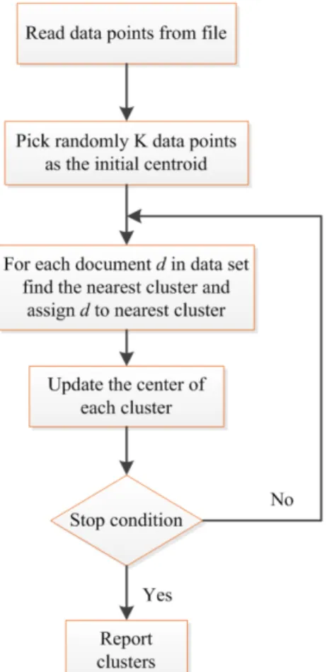
In the general sense, flat clustering techniques separate data into a prespecified number of mutually exclusive and exhaustive groups (clusters). Most algorithms that produce flat clustering are iterative. They start with a set of initial clusters and improve them by iterating over a reallocation operation that reassigns objects. K-means is the best known partitioning algorithm [McQueen, 1967]. The K-means algorithm partitions the given data into K clusters. It is common to pick K data points at random or just pick the first data, as the initial cluster centers (centroids). The algorithm then assigns each data point to the nearest center. The updating and reassigning process can be kept until a convergence criterion is met. For updating each centroid, just recomputed the center of each cluster or the mean value of its members as the centroid. The algorithm converges when there is no further change in the assignment of instances to the clusters. Figure 2-1 depicts the flowchart of the K-means method.

(21)

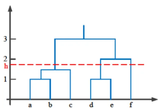
7 The second group of clustering approaches is hierarchical clustering techniques that produce a tree also called dendrogram. They avoid specifying the number of clusters and provide a partition for each point obtained from cutting the tree at some level. This partitioning needs the use of a similarity measure, or equivalently a distance measure, defined between instances. Figure 2-2 illustrates the hierarchical clustering structure [Manning and Schutze, 1999].

Figure 2-2: The dendrogram of the hierarchical clustering method.

As seen in Figure 2-2, a hierarchical cluster is a hierarchy where each node stands for a subclass of its mother’s node. The leaves of the tree are the single objects of the clustered set. Each node represents the cluster that contains its children. The clustering tree can be built in two distinct ways: bottom-up (agglomerative clustering) and top-down (divisive clustering). An agglomerative clustering algorithm starts with N groups, each initially containing one training instance, merging similar groups to form larger groups and moving up hierarchically, until there is a single one. At each iteration of the agglomerative algorithm, the two closest groups considering a measure are chosen to merge. A divisive clustering algorithm goes in the other direction, starting with a single group and dividing large groups into smaller groups, until each group contains a single instance. Choosing hierarchical clustering is suitable for detailed data analysis and it provides more information than flat clustering [Manning and Schutze, 1999].

(22)

8

2.2

Probabilistic language models

Language modeling could be considered as an example of statistical estimation where the problem is to predict the probability of a word given the probability of previous words and sometimes the probability of some following words. To have a precise estimate for model parameters, a language model must be trained on a large corpus of text. Accurate language modeling is essential in speech or optical character recognition, spelling correction, handwriting recognition, statistical machine translation and word segmentation [Manning and Schutze, 1999]. This task has been discussed in Shannon game for guessing the next letter in a text [Shannon, 1951]. As is well known, the word prediction task is a well understood problem for which several techniques could be developed. N-gram and Multigram are two important language modeling approaches which are widely used in artificial intelligence and natural language processing. The following sections discuss these two models in more details.

2.2.1 N-gram models

Generally, an N-gram is a sequence of N words appearing consecutively in some corpus. The distribution of the N-grams encountered in a training corpus forms a language model that can be applied to predict the next words. It can estimate the probability of each word by using the probability of the N-1 prior words. If w1n =w w1... n is defined as the word sequence, the prediction task can be considered as a conditional probability problem

1 1

( | ,...,n n )

P w w w− . For practical applications, N-grams models with N =1, 2, 3 and 4 are

the most frequent, and they are respectively called unigram, bigram, trigram and four-gram models. The conditional probability P w w( | ,..., )n ₁ wn of an N-gram can be expressed by:

(

)

1 1 1 1 1 1 1 1 ( , , ) ( , , ( , , ) ) ) ( n n n n n n P w w P w P w |w w P w w P w − − − … … = = … (2.1)

(23)

9 where P w w( , , )1 … n is the joint probability between w w1... n−1 and wn . Applying the

general probability chain rule, the conditional probability of an N-gram becomes:

2 1 1 1 1 2 1 3 1 1 1 1 ( )n ( ) ( | ) ( | )... ( | n ) n ( | k ) n k k P w P w P w w P w w P w w − P w w − = = =

∏

(2.2)

Assuming that the occurrence of wn can only be influenced by the preceding N-1 words,

the conditional probability can be approximated as:

1 1 1 1 ( )n n ( | k ) k k N k P w P w w − − + = =

∏

(2.3)

For bigrams, this expression corresponds to:

1 1 1 ( )n n ( | ) k k k P w P w w− = =

∏

(2.4)

N-gram conditional probabilities can be estimated from raw text based on the relative frequency C of word sequences [Russell and Norvig, 2010]. In the case of bigram:

1 1 1 ( ) ( | ) ( ) n n n n n C w w P w w C w− − − = (2.5)

and in the more general N-gram case:

1 1 1 1 1 1 ( ) ( | ) ( ) n n n N n n n N n n N C w w P w w C w − − − + − + − − + = _(2.6)

Performance of N-gram models can be evaluated based on their abilities to predict the words probabilities. In the literature, several measures have been proposed to assess the N-gram model performance such as perplexity, recall and precision [Manning and Schutze, 1999].

(24)

10

2.2.2 Multigram

Typically, an N-gram model is used for language modeling purpose. It assumes that the probability of one word in a document depends on its preceding N − words where N is a 1 fixed value for all text. Conversely, an N-multigram model [Deligne and Bimbot, 1995; Deligne and Bimbot, 1997] assumes that a sentence is a concatenation of independent variable-length sequences of words and the number of words in each sequence is at most

N. As an example, let W be all possible vocabularies, and let w w w= ₁, ,...,₂ w₄ be a sentence defined on this vocabulary, where w Wi∈ and i = 1 4. In a Multigram framework, the

sentence w has the set of all possible segmentations of the sentence associated to it. Let S be this set of segmentations for w. If we use the symbol # to express the concatenation of words which constitutes the same segment, S is expressed as follow:

1 2 3 4 1 2 3 4 1 2 3 4 1 2 3 4 1 2 3 4 1 2 3 4 1 2 3 4 1 2 3 4 , # , # , # , # # , # # , # # , # # # w w w w w w w w w w w w w w w w S w w w w w w w w w w w w w w w w       =         (2.7)

In Multigram language modeling context, the likelihood of a sentence is computed by summing up the likelihood values of all possible segmentations of the sentence. The likelihood of the sentence L w( ) given a Multigram model is:

( ) ( , )

s S

L w L w s

∈

=

∑

_(2.8)

where L w s( , ) is the likelihood of the sentence w given the segmentation s. This approach

could be seen as an extension of N-gram models.

In this study we use Multigram models for estimating the probability of words. Since a specific format of Baum-Welch algorithm is used for training the Multigram models, the general ideas underlying Baum-Welch algorithm are presented in following section, while its adopted version for word segmentation problem will be discussed in chapter 3 with more details.

(25)

11 Baum-Welch Algorithm

Baum Welch algorithm is usually applied for learning with Hidden Markov Model (HMM) [Baum, 1972]. In HMM, given some observed sequences O, the objective of learning a model is to identify the parameters µ =( , , )A B π , where A and B stand for state transition and observation probability matrices, and π represents the initial state. As opposed to Markov chain, it is impossible for a HMM to directly calculate the model parameters, since we don’t know which path of states was taken through the machine for a given input. In this regard, a Maximum Likelihood estimator is utilized to estimate the model parameters. In fact, it finds the model values that maximize the probability of an observation O, i.e.

(

)

ˆ max ( | )P O

µ

µ = µ . This goal can be achieved by using Baum-Welch, also called forward-backward algorithm, which is a special case of the Expectation Maximization method [Manning and Schutze, 1999]. Given sequence of observation O={ , , , ,o o1 2  o ot t+1, , } oT ,

Baum-welch algorithm has one initialization and three main steps that are preformed recursively.

Step 0: Initialization

In this step, model parameters µ=( , , )A B π are initialized using random values taken from possible ranges.

Step 1: Forward procedure

Here, the probability of seeing { , , , }o o1 2  ot and being in state i at time t (αi( )t ) is calculated. In other words, for each time t, we try to find the probability of:

(

1 1

)

( ) , , , |

i t P O o O o Xt t t i

α = = _ = = µ (2.9)

To do so, a recursive calculation is used:

1 ( ) ( ) N ( 1) j j t i i j i t b o t a α α = =

∑

− × (2.10) where

(26)

12

1

(1) ( )

i i jb o

α =π (2.11)

and ( )b o is the probability of a certain observation vector at time t for state j given by j t

( ) ( | )

j t t t t

b o =P O o X= = (2.12) j

While a as an element of transition matrix is defined as: i j

1

( | )

i j t t

a =P X = j X − = i (2.13)

Step 2: Backward procedure

In this step, βi( )t =P O

(

t+1=ot+1, ,OT =o XT | t =i,µ

)

as the probability of the ending partial sequence {ot+1, , } oT given starting state i and time t is calculated.

1 1 ( ) N ( 1) ( ) i j i j j t j t t a b o β β ₊ = =

∑

+ × × _(2.14) where ( ) 1 i T β = (2.15)

Step 3: Update model parameters

To update the parameters, we should first calculate some temporary variables γi( )t and ( )

i j t

ξ . γi( )t is the probability of being in state i at time t given the observed sequence O and model µ.

(

)

1 ( ) ( ) ( ) | , ( ) ( ) i i i t N j j j t t t P X i O t t α β γ µ α β = = = =

∑

(2.16)

Also, ( )ξi j t , as the probability of being in state i and j at times t and t+1 respectively given

(27)

13

(

)

1 1 1 1 1 ( ) ( 1) ( ) ( ) , | , ( ) ( 1) ( ) i i j j j t i j t t N N k km m m t k m t a t b o t P X i X j O t a t b o α β ξ µ α β + + + = = + = = = = +

∑∑

(2.17)

Now, we are able to update model parameters (µˆ =( , , )A Bˆ ˆ πˆ ):

ˆi i(1)

π =γ (2.18) which is the expected frequency spent in state i at time 1.

1 1 1 1 ( ) ˆ ( ) T i j t i j T i t t a t ξ γ − = − = =

∑

(2.19)

In fact, ˆa is calculated using the expected number of transitions from state i to state j i j compared to the expected total number of transitions away from state i. Observation matrix is updated as: 1 1 ( ) ˆ ( ) ( ) t k T o v i t i k T i t t b v t φ γ γ = = = × =

∑

(2.20)

where φo v_t=_k is an indicator function expressed as:

1, if 0, otherwise t k t k o v o v φ ₌ _{= } =  (2.21)

In other words, b vˆ ( )i k is calculated using the expected number of times that the output

observations have been equal to vk while in state i over the expected total number of times in state i. Baum-welch algorithm iteratively repeats steps 1, 2, and 3 until convergence is reached. The basic idea of Baum-Welch is presented in Figure 2-3.

(28)

14 Hidden states 1 2 j i N t-1 t t+1 t+2 T Time

{

( )1 ij j t a b o+ ( ) i t α β_j( 1)t+

Figure 2-3: The probability of traversing an arc from state i to j: the α and β probabilities, the transition probability aijand the observation probability b oj( t+1) [Jurafsky and Martin, 2000].

2.3

Word Segmentation

Text segmentation is the process of dividing a text into meaningful units that could be words, sentences, paragraphs or topics. As a specific case, word segmentation is defined as the problem of dividing a string of written language into its component words and it is wildly used in natural language processing applications [Manning and Schutze, 1999]. This problem is non-trivial, because while some written languages have explicit word boundary markers, such as the word spaces of written English and the distinctive initial, medial and final letter shapes of Arabic, such signals are sometimes ambiguous and not present in all written languages. In English and many other languages using some form of the Latin alphabet, the space and punctuation is a good approximation of a word delimiter.

2.3.1 Problems in Word Segmentation

Many languages include major East-Asian languages/scripts, such as Chinese, Japanese, and Thai do not put spaces between words at all, and so word segmentation algorithm could be a challenging task in such languages [Gao et al., 2005; Hua, 2000]. As mentioned

(29)

15 before, whitespace is a good approximation for word segmentation but it is not signifying a word break. For example, a word can be accompanied by punctuation or some special symbols. In most cases, the problem has been solved by dealing with building carefully handcrafted regular expressions to match formats, but this kind of regular expressions does not cover all the problems. For example, when a word is compound like database, we may wish to regard them as a single word like data and set. Also, for phone numbers like 418 656 2131 each part counts as a single word. In multi part name like New York or Quebec City, or in phrasal verb such as make up, work out, this problem masks more complicated and difficult issues for the task of segmentation. An unsegment text can be assumed similar to the world which is too complex to be considered all at once, both computationally and conceptually. Instead, it must be broken into manageable pieces, or chunks, and dealt with one piece at a time. However, this is not a trivial task for new domains. It isn’t clear what segmentation strategy one should use, or even what metric should be used to evaluate the quality of a segmentation.

To explain the word segmentation, imagine you are reading some text like this: ”COULDYOUTELLMEWHATYOUTHINKABOUTFUTURE” and you know nothing about the language. How would you segment such a continuous stream of letters into words? This is the task that word induction is trying to solve: automatically discovering words from only text with no word boundary information.

Obviously, automatic word segmentation needs wide linguistic knowledge. In linguistics context, the description of a language is split into two parts, the grammar consisting of rules describing correct sentence formation and the lexicon listing words and phrases that can be used in the sentences. So it can be said that the lexicon of a language is its vocabulary. More specifically, in NLP context, a lexicon is a dictionary that contains all possible words (meaningful or not) constructed based on language alphabets.

2.3.2 Word Segmentation Approaches

In the literature, many word segmentation methods have been proposed and discussed [Hua, 2000; Nevill-Manning and Witten, 1997]. In the following section, Voting Experts

(30)

16

(VE) and Sequitur techniques, two well-known unsupervised word segmentation algorithms, will be presented and the related concepts will be discussed.

Voting Experts

Voting Experts is an algorithm for the unsupervised segmentation of discrete token sequences. It was first suggested by Paul Cohen [Cohen et al., 2007; Hewlett and Cohen, 2009] and it has been shown to be proficient for segmenting large text corpora where all spaces and punctuation marks have been removed. The result of running the VE algorithm on the ﬁrst 500 characters of the book 1984 is shown below. The * symbols are induced boundaries:

Itwas * a * bright * cold * day * in * April * andthe * clockswere * st * ri * king * thi * rteen * Winston * Smith * his * chin * nuzzl * edinto * his * brea * st * in * aneﬀort * to * escape * the * vilewind * slipped * quickly * through * the * glass * door * sof * Victory * Mansions * though * not * quickly * en * ought * oprevent * aswirl * ofgrit * tydust * from * ent * er * inga * long * with * himThe * hall * ways * meltof * boiled * cabbage * and * old * ragmatsA * tone * endof * it * acoloured * poster * too * large * for * indoor * dis * play * hadbeen * tack * ed * tothe * wall * It * depicted * simplya * n * enormous * face * more * than * ametre * widethe * faceof * aman * of * about * fortyﬁve * witha * heavy * black * moustache * and * rugged * ly * handsome * featur

The Voting Experts algorithm uses a set of ’experts’, rules for deciding where to place segment boundaries [Miller and Stoytchev, 2008]. The algorithm moves a sliding window of a fixed size over the sequence of symbols. At each position of the window, each expert votes on the most likely segment boundary within the current window. Then, the algorithm traverses the sequence of symbols, and introduces segment boundaries where the sum of votes for the next position is smaller than the sum of votes for the current position.

The VE algorithm uses two set of experts defined based on internal entropy and boundary entropy [Miller and Stoytchev, 2008]. From a VE point of view, chunks are composed of elements that are frequently found together, and that are found together in many different circumstances. VE looks for these two properties and uses them to segment text. To find

(31)

17 the possible boundary locations, one expert votes to place boundaries after sequences (seq) that have low internal entropy HI given by:

( )

log (

(

)

I

H seq = − P seq (2.22)

where P is the probability of the seq. The other places vote after sequences that have high boundary entropy HB, given by

( )

( | ) log ( |

(

)

B _{c S}

H seq =

∑

_∈ P c seq × P c seq (2.23)

where S is the set of successors to seq. All sequences are evaluated locally, within a sliding window, allowing the algorithm to be very efficient.

The statistics required to calculate HI and HB are stored efficiently using proper data

structure, which can be constructed in a single pass over the corpus. The sliding window is passed over the corpus, and each expert votes once per window for the boundary location that best matches that expert’s criteria. After voting is complete, the algorithm yields an array of vote counts, each element of which is the number of times some expert voted to segment at that location. The result of voting on the string thisisadog could be represented in the following way t0h0i1s3i1s4a4d1o0g, where the number between each letter is the number of votes that location received.

With the final total votes in place, the final segmentation consists of the locations that meet two requirements: first, the number of votes must be locally maximal (also called the zero crossing rule). Second, the number of votes must exceed a chosen threshold. Thus, Voting Experts has three parameters: the window size, the vote threshold, and whether to enforce the zero crossing rules.

Sequitur

Sequitur establishes a grammar for a given sequence based on repeated phrases in that sequence [Nevill-Manning and Witten, 1997a; Nevill-Manning, and Witten, 1997b]. Each

(32)

18

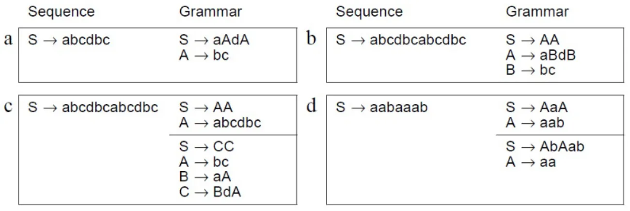
repetition leads to a rule in the grammar, and the repeated subsequence is replaced by a nonterminal symbol, producing a more brief representation of the overall sequence. The concept of Sequitur approach is illustrated for a given sequence in Figure 4. In Figure 2-4(a), a sequence that contains the repeating string bc has been identified. To compress the sequence, Sequitur forms a new rule A→bc, and A replaces both occurrences of bc. The

right side of Figure 2-4(a) shows the new grammar.

Figure 2-4(b) shows how rules can be reused in longer rules. The longer sequence contains two copies of the sequence in Figure 2-4(a). Since there is an exact repetition, the sequence can be compressed by forming the rule A→abcdbc. To achieve more compressed format, rule B→bc can be defined. This demonstrates the advantage of treating the sequence, rule

S, as part of the grammar. More precisely, rules may be formed from rule A in the same

manner to rules formed from rule S. The grammar’s hierarchical structure is formed by using these rules. As shown in Figures 2.4(a) and 2.4(b), the grammars have two common properties:

• p₁: no pair of adjacent symbols appears more than once in the grammar. • p₂: every rule is used more than once.

Property p1 requires that every diagram in the grammar be unique. It is called the diagram

uniqueness. Property p₂ guarantees that each rule is useful, this property is named utility rule. In Sequitur, a generated grammar is characterized by these two constraints.

Figure 2-4(c) shows what happens when these properties are violated. The first grammar contains two occurrences of bc, so p1 is not satisfied and this introduces redundancy

because bc appears twice. In the second grammar, rule B is used only once, so p2does not

hold. If it is removed, the grammar would become more concise. In Figures 2.4(a) and 2.4(b), the grammars are the only ones for which both properties are satisfied for each sequence. However, applying these properties can lead to different and correct grammars. For example, Figure 2-4(d) represents two grammars for a given sequence which they both

(33)

19 obey p1 and p2. So each of them is acceptable. Repetitions cannot overlap, so the string

aaa does not give rise to any rule, despite containing two diagrams aa.

Sequitur approach checks that both properties hold for each ruling. In other words, these properties are applied as the constraints in this algorithm, and it operates by enforcing the constraints on a grammar. When the diagram uniqueness constraint is violated, a new rule is formed. When the rule utility constraint is violated, the useless rule is deleted.

Figure 2-4: Example sequences and grammars that reproduce them: (a) a sequence with one

repetition; (b) a sequence with a nested repetition; (c) two grammars that violate the two constraints; (d) two different grammars for the same sequence that obey the constraints

[Nevill-Manning and Witten, 1997a].

2.4

Optimization algorithm

Optimization can be simply defined as the process of making something better. Optimization helps a scientist to improve his ideas by gaining new information. One can feed some data into the optimization approach, and then get the solution, but this solution should be investigated and interpreted. There are a lot of issues that should be addressed by optimization methods. Is this the only solution? Is it the best solution? What is the cost of finding a better solution? In this section, Viterbi approach and genetic algorithms (GA), and some of their applications in engineering and computer science fields will be presented. Here, genetics algorithm is described as one of the most known meta-heuristic

(34)

20

optimization approach, and also to prepare an introduction for another meta-heuristic algorithm, Harmony Search, which will be extensively investigated in the next chapters. In general, an optimization problem is defined by using two set of equations: an objective function and some constraints. An objective function, also called cost, energy or fitness function is the equation that the optimizer attempts to minimize/maximize and its definition depends on the optimizer’s goals and problem nature. Constraints, also called model, indicate the search space, i.e. the region where an optimal solution can be found (feasibility region). Therefore, an optimization problem can be formulated as:

(

)

* _{arg min/ arg max} _{( )}

x

x = F x (2.24)

subject to

x S∈ (2.25)

where x is the optimization variable set, F and S stand for the objective function and

constraints, respectively. According to the objective function and the characteristics of constraints, optimization approaches can be classified in different categories. Figure 2-5 [Haupt and Haupt, 2004] shows the main six main categories of optimization algorithms. It should be noted that these six classes are not necessarily separated from each other. For instance, a dynamic optimization problem could be discrete or continuous.

2.4.1 Viterbi

Viterbi is a dynamic programming algorithm that computes the most likely state transition path given an observed sequence of symbols [Ryan and Nudd, 1993]. Let q q q= 1 2qT be

a sequence of states. The objective is to find:

(

)

* _,

q

q =argmax p q|O λ (2.26)

where O and λ are respectively the observation set and a given model. Viterbi algorithm grows the optimal path q* gradually while scanning each of the observed symbols. At time

(35)

21

t, it keeps track of all the optimal paths ending at each of N different states. At time t+1, it

then updates these N optimal paths. The algorithm will be elaborated in Chapter 3.

Figure 2-5: The six main categories of optimization algorithms [Haupt and Haupt, 2004].

2.4.2 Genetic algorithm and application

In many nonlinear optimization problems where analytical optimization methods are not normally applicable, the objective function has a large number of local minima and maxima and so finding the global minimum (or maximum) is really problematic. In this situation, the use of deterministic optimization techniques often leads to hard challenges. In order to overcome the computational drawback of mathematical techniques, meta-heuristic optimization algorithms have been proposed. These algorithms explore the search space using different methods in order to find (near-) optimal solutions with less mathematic efforts. Generally, meta-heuristic algorithms are approximate and non-deterministic for solving complex optimization problems in business, commerce, engineering, industry, computer science, etc. Meta-heuristic algorithms have two mutual aspects: rules and randomness to mimic natural phenomena [Lee & Geem, 2005]. According to these two,

(36)

22

different types of meta-heuristic search techniques have been proposed. Consequently, they could be categorized from several points of view. Evolutionary algorithms (EA) are the biggest group of meta-heuristic algorithms. This category contains genetic algorithm (GA) and Harmony Search (HS) approach that are investigated in the following section and the fourth chapter of this thesis.

GA generates solutions for optimization problems using techniques inspired by natural evolution, such as inheritance, mutation, selection, and crossover. The idea of genetic algorithm appeared first in Bagleys [1967]. The theory and applicability was then strongly influenced by J. H. Holland, who can be considered as the pioneer of genetic algorithms [Holland, 1992a] and further developed by Goldberg [Loganathan, 2001] and others. Since then, this field has witnessed a tremendous development.

There are many applications where genetic algorithms are used. A wide spectrum of problems from various branches of knowledge can be considered as optimization problem. These problems appear in economics and finances, cybernetics and process control, engineering fields [Haupt and Haupt, 2004]. It could be applied to continuous or discrete optimization problem and it does not require any derivative information. Moreover, it is able to deal with a large number of variables and it is well suited for parallel computations. GA has applications in computer science for example game theory, pattern recognition and image analysis, cluster analysis, natural language tagging [Alba et al., 2006], story segmentation [Wu et al., 2009], image segmentation [Andrey and Tarroux, 1994], robot trajectory planning [Davidor, 1991].

Before going through the approach, it seems essential to give some basic definitions related to the approach:

• Gene xi is a single encoding part of the solution space, i.e. either single bits

or short blocks of adjacent bits that encode an element of the candidate solution. • Chromosome x called genome or individual is a set of parameters (genes) that represents a possible solution to the problem that the GA is trying to solve. In other words, a chromosome is a solution vector. In most cases, the chromosome is

(37)

23 represented as a simple string. Although a wide variety of other data structures are also used.

• Population N is the number of chromosomes available to test. The population size depends on the nature of the problem.

• Fitness function F x( ) is a particular type of objective function that is used

to summarize, as a single figure of merit, how close a given design solution is to achieving the set aims. In GA context, the fitness function is used to select the chromosomes i.e. finding the best solution.

As already mentioned, the GA imitates the natural evolution and inheritance between generations. The main core of the GA is the procedure called reproduction which transfers information from one generation to other one. Generally, this procedure has three steps: a) Selection, b) Crossover and c) Mutation. In fact, the GA creates a new generation by using these operators and past generations.

a) Selection

The selection algorithm determines which individuals (chromosomes) will belong to the new generation. The probability of an individual to be selected for the next generation increases with the fitness of the individual being greater or less than its competitor’s fitness. There are many selection methods such as Roulette wheel selection, deterministic sampling, and stochastic remainder sampling described as below:

• In the Roulette method [Goldbarg, 2000], also known as fitness proportionate selection, the first step is to calculate the cumulative fitness of the whole population through the sum of the fitness of all chromosomes. After that, the probability of selection P is calculated for each chromosome as being sel_i

1 i N sel i i i P F F =

=

∑

where Fi presents the value of the fitness function for the ith chromosome. Then, an array is built containing the cumulative probabilities of the individuals. So, n random numbers are generated within the range 0 to

∑

F_i and,

(38)

24

for each random number, an array element that can have higher value is searched for. Therefore, individuals are selected according to their probabilities of selection. • In deterministic sampling [Brindle, 1981], the average fitness of the population is calculated and the fitness associated to each individual is divided by the average fitness, but only the integer part of this operation is stored. If the value is equal or higher than one, the individual is copied to the next generation. The remaining free places in the new population will be filled with chromosomes with the greatest fraction.

• The stochastic remainder sampling [Brindle, 1981] has concepts identical to those used in the deterministic sampling. The only difference between them is that for the stochastic approach, free places were filled based on the roulette method. b) Crossover

In genetic algorithm context, crossover is an operator used to vary the programming of a chromosome or chromosomes from one generation to the next. It is analogous to reproduction and biological crossover, upon which genetic algorithms are based. Crossover combines two chromosomes (parents) to produce a new chromosome (offspring). The idea behind crossover is that the new chromosome may be better than both of the parents if it takes the best characteristics from each of the parents. Crossover occurs during evolution according to a user-definable crossover probability. There are many ways of doing the crossover [Sivanandam, 2008], such as the one-point, the two-point, and the uniform crossover explained below.

In the one-point crossover, a random number defines the segment reference that splits off the chromosome into two parts. The children are generated through the region combination (generated by the segment point) of the two parents, selecting genetic material belonging to one and another parent in an alternating way (Figure 2-6).

(39)

25

Figure 2-6: One-point crossover

A variation of this method, known as the two-point crossover, consists in considering two segmentations of the chromosome (instead of only one). In this case, everything between the two points is swapped between the parent organisms, rendering two child organisms (Figure 2-7).

Figure 2-7: Two-point crossover

The uniform crossover uses a fixed mixing ratio between two parents. Unlike one and two-point crossover, the uniform crossover enables the parent chromosomes to contribute at the gene level rather than at the segment level. If the mixing ratio is 0.5, the offspring has approximately half of the genes from first parent and the other half from second parent, although cross over points can be randomly chosen (Figure 2-8).

Crossover point Parents: Children: Crossover points Parents: Children:

(40)

26

Figure 2-8: Uniform crossover

c) Mutation

In genetic algorithms, mutation is an operator used to keep genetic diversity from one generation of a population of chromosomes to the next [Holland, 1992b]. Mutation alters one or more gene values in a chromosome from its initial state. In mutation, the solutions may change entirely from the previous solution. Therefore GA can come to better solution by using mutation. Mutation occurs during evolution according to a user-definable mutation rate or probability. More precisely, mutation rate determines that a given chromosome should be randomly replaced or not. This threshold should be set low, since if it is set too high, the search will turn into a primitive random search.

A common method of implementing the mutation operator involves generating a random variable for each bit in a sequence. This random variable tells whether or not a particular bit will be modified. This mutation procedure, based on the biological point mutation, is called single point mutation. Other types are inversion and floating point mutation. When the gene encoding is restrictive as in permutation problems, mutations are swaps, inversions and scrambles. Mutation should allow the algorithm to avoid local minima by preventing the population of chromosomes from becoming too similar to each other, thus slowing or even stopping evolution.

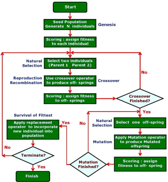
Once the genetic representation of the problem and the fitness function are defined, genetic algorithm can proceed as follow. Figure 2-9 present a flowchart of genetic algorithm implementation.

Parents:

(41)

27 1. [Start] Generate a random population of N chromosomes (i.e. possible

solutions for the problem).

2. [Fitness] Evaluate the fitness F(x) of each chromosome x in the population. 3. [New population] Create a new population by repeating the following steps

until the new population is complete.

a) [Selection] Select two parent chromosomes from a population according to their fitness (better the fitness, bigger the chance to be selected).

b) [Crossover] With some crossover probability, crossover the parents to form new offsprings (children).

c) [Mutation] With a mutation probability, mutate each new offspring at each locus (position in chromosome).

d) [Accepting] Place new offsprings in the new population.

4. [Replace] Use the new generated population for a further run of the algorithm. 5. [Test] If the end condition is satisfied, stop, and return the best solution in the

current population. 6. [Loop] Go to step 2.

Types of genetic algorithms

In addition to standard GA, depending on different applications and problems, different types of GA have been proposed in literature. This section briefly explains two types of GA which are commonly used in computer science context: Binary genetic algorithm and Continuous genetic algorithm.

Binary genetic algorithm

Binary genetic algorithm (BGA) can be considered as a specific case of discrete genetic algorithm where optimization variables are discrete, and objective function and constraints are defined for discrete space [Haupt and Haupt, 2004]. In BGA, since genes can only take

(42)

28

1 or 0, chromosomes are sequence of binary digits. In this case, the fitness functions should be defined so that they are able to quantify these binary strings. In other words, cost function should be able to convert discrete variables (discrete events) to continuous values and vice versa. In the literature, several quantizing techniques have been introduced such as clustering and rounding the value to the low or high value, Table 2-1 shows an example for decoding a gene in a binary chromosome.

(43)

29

Table 2-1: Decoding a gene in Binary genetic algorithm

Binary

Representation Decimal First Number Quantized x First Quantized x Second Color Opinion

00 0 1 1.375 Red Excellent

01 1 2 2.125 Green Good

10 2 3 2.875 Blue Average

11 3 4 3.625 Yellow Poor

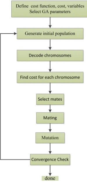
In binary GA, the population matrix is filled by random value 0 or 1. At first, random numbers are generated between 0 and 1, and then they are rounded to the closest integer 0 or 1. Each row represents a chromosome. Approaches of selection, mating, mutation and convergence are chosen depending on the problems. For instance, a simple method for mutation is just changing a 1 to a 0, and vice versa. Figure 2-10 illustrates the general procedure of binary GA.

Continuous Genetic Algorithm

The binary GA can solve many optimization problems but there are some limitations in the quantization step. When an optimization problem contains many variables, so the size of the chromosome will be very large, 1s and 0s are not the good way to represent these variables that require many bits. For example, 50 variables lead to a _{50 2}_× 6_{bits length} chromosome. In Continuous GA (CGA), since all variables are continuous, constraints and objective function are defined on continuous domain. And consequently there is no need to quantize the variables [Haupt and Haupt, 2004]. CGA has two main advantages:

a) It requires less storage space than BGA, and

b) It is faster than BGA, because as seen in Figure 2-11, the chromosomes do not need to be decoded for calculating the fitness function.

(44)

30

In Figure 2-11, the general procedure of continuous GA is illustrated. It is noticeable that in continuous GA context, various approaches have been proposed in the literature for selection, mating, mutation and convergence.

(45)

31

Figure 2-11: General procedure of a continuous genetic algorithm

2.5 Summary

In this chapter, first supervised and unsupervised learning techniques have been first discussed. Then probabilistic language models including N-gram and muligram have been elaborated and related details were presented. As the third section, word segmentation was presented in natural language processing context. Two unsupervised word segmentation approaches, Voting Experts and Sequitur, have been described in details. In the last section, optimization algorithms including Viterbi and genetic algorithms have been illustrated and different types of GA have been discussed.

(46)

(47)

33

Chapter 3. Unsupervised Hierarchical Segmentation using Viterbi

Algorithm

This chapter presents an unsupervised probabilistic word segmentation technique called Unsupervised Hierarchical Segmentation (UHS). This segmentation approach is described step by step and related issues are discussed. This chapter provides a thorough description of how UHS algorithm selects word boundaries within a text containing no separators such as white spaces and punctuation marks.

3.1

General framework

This section presents an unsupervised learning algorithm [Shani et al., 2009] that segments sequences of categorical events or letters. The algorithm hierarchically builds a set of all the possible chunks that can happen in the text and save them in a lexicon. Then it finds the best segmentation from the sequence of characters using the lexicon. This technique proceeds by creating a hierarchical segmentation structure, where smaller segments are grouped into larger segments. Generally, UHS algorithm contains three main phases: 1) A lexicon of meaningful segments is built.

2) The probabilistic model over the given lexicon is trained.

3) The sequence of events is segmented using the given lexicon and model.

These phases are repeated iteratively to incrementally build a hierarchical lexicon and create a hierarchical segmentation of the sequence.

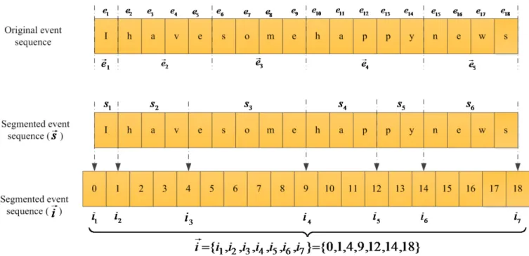
Before going deeper into the details of the algorithm, it is vital to establish a correct notation and a clear definition for word segmentation problems [Shani et al., 2009]. In this context, a sequence of discrete events ("letters") is denoted by:

1, , ,2 n

(48)

34

where belongs to a finite known alphabet . A set of m sequences is expressed by: (3.2)

A segmentation of is represented by , which is a sequence of indices where and . sj is defined as the segment in the sequence and it can be

simply expressed as:

(3.3)

In fact, the segment boundary is placed after the segmentation index. Using a segmentation for a given event sequence , a segment sequence could be expressed by:

(3.4)

The set of all possible segments is called the lexicon, denoted by S. Figure 3-1 is an example for showing the meaning of these notations. The vertical dashed lines show the boundaries of segments. In the first line, the original event sequence (text) is presented, while next lines show a segmentation and corresponding notations.

(49)

35 Figure 3-2 illustrates the flowchart of the unsupervised hierarchical segmentation algorithm. First, the lexicon is initialized by the single letters of the alphabet. Then raw text, which is obtained by removing white spaces, punctuations, special characters and numbers form the original text, is used to initialize the segmentation.

Figure 3-2: General flowchart of UHS using Viterbi

Figure 3-3 shows the main interaction cycle in UHS approach. The method recursively performs three main tasks. First it builds a lexicon. Second it builds the model and then segments the sequence at each iteration. The USH algorithm is presented in Figure 3-4. In the next sections we will explain the method step by step with more details.

(50)

36

Figure 3-3: The cycle of interaction in UHS

Algorithm: Unsupervised hierarchical segmentation using Viterbi input η←{ , , , }e e₁ ₂…em

input δ←MIthreshold

I ←0 // Iteration number

η₀←η //The first segmentation is the raw text

L0← Ση//The initial lexicon by all letters of the alphabet

while δ ε> do //Epsilon is the minimum value to stop the procedure I← +I 1

L_I←L_I₋₁

//Add concatenation of two successive segments to the lexicon if mutual information exceeds δ for each consecutive chunks in segment

if MI (e e ) >δ then 1 2

Add e e to 1 2 L I end if

end for

//Create the new multigram over new lexicon Initialize a multigram M using lexicon LI

Train M on η_I using the Baum-Welch algorithm

//Segment the sequence using the new multigram for j = 0 to m do

Add the most likely segmentation of ejgiven M to ηI+1

end for

δ←δ₂

end while Output η_I−₁

(51)

37

3.2 Phase 1 - Build Lexicon

During the first phase of the UHS approach, a lexicon is built from all possible chunks that occur more often in the text. To illustrate how the lexicon is built, we will use a text written in English in the next sections.

To initialize the approach and corresponding parameters, some preparation steps are needed. First all punctuations, numbers and other symbols are removed from the text. Then all capital letters are turned into lowercase. The sequence of characters is then ready to initialize the segments, i.e. raw prepared text is used as the first segments.

In the UHS approach, all the letters of the alphabet are considered at the first level of the lexicon. It is noticeable that the content of the lexicon is always sorted by alphabetic order. At each iteration, after adding new elements to the lexicon, it is sorted again. The following sub-sections explain the meaning and structure of a hierarchical lexicon and how it can be built.

3.2.1 Hierarchical lexicon structure

The UHS algorithm benefits from a lexicon that is hierarchically and iteratively updated. The main reasons for the significant attention to hierarchical lexicon structures are the fact that redundancy in the lexicon is avoided. Van der Linden [1992] discussed hierarchical lexicons in the context of Natural Language Processing. This special form of lexicon plays an essential role in the success of UHS. Therefore, the current section is devoted explaining the structure of the hierarchical lexicon by using a visual example. As mentioned above, the lexicon is first initialized with alphabet letters. Then if the association between two successive segments, measured by mutual information, is more than a predefined threshold, they are concatenated and added at a higher level of the lexicon.

Unsupervised segmentation of sequences using harmony search and hierarchical clustering techniques