HAL Id: inria-00352032
https://hal.inria.fr/inria-00352032
Submitted on 12 Jan 2009
HAL is a multi-disciplinary open access
archive for the deposit and dissemination of
sci-entific research documents, whether they are
pub-lished or not. The documents may come from
teaching and research institutions in France or
abroad, or from public or private research centers.
L’archive ouverte pluridisciplinaire HAL, est
destinée au dépôt et à la diffusion de documents
scientifiques de niveau recherche, publiés ou non,
émanant des établissements d’enseignement et de
recherche français ou étrangers, des laboratoires
publics ou privés.
Visual servoing from 3D straight lines with central
catadioptric cameras
Youcef Mezouar, Hicham Hadj-Abdelkader, P. Martinet, François Chaumette
To cite this version:
Youcef Mezouar, Hicham Hadj-Abdelkader, P. Martinet, François Chaumette. Visual servoing from
3D straight lines with central catadioptric cameras. Fifth Workshop on Omnidirectional Vision,
Om-nivis’2004, 2004, Prague, Czech Republic, Czech Republic. �inria-00352032�
Visual Servoing From 3D Straight Lines
With Central Catadioptric Cameras
Y. Mezouar1, H. Hadj Abdelkader1, P. Martinet1, and F. Chaumette2
1 LASMEA, 24 avenue des Landais, 63177 Aubi`ere-France
{mezouar, hadj, martinet}@lasmea.univ-bpclermont.fr
2 IRISA Campus de Beaulieu, Rennes-France
Abstract. In this paper we consider the problem of controlling the six degrees of freedom of a manipulator using the projection of 3D lines in the image plane of central catadioptric systems. Most of the effort in visual servoing are devoted to points, only few works have investigated the use of lines in visual servoing with traditional cameras and none has explored the case of omnidirectional cameras. First a generic interaction matrix for the projection of 3D straight lines is derived from the projection model of the entire class of central catadioptric cameras. Then an image-based control law is designed and validated through simulation results.
1
Introduction
In the last years, the use of visual observations to control the motions of robots has been extensively studied (approach referred in the literature as visual ser-voing). Computer vision can provide to the robotic system a powerful way of sensing the environment and can potentially reduce or obliterate the need for environmental modeling, which is extremely important when the robotic tasks require the robot to move in unknown and/or dynamic environments.
Conventional cameras suffer from restricted field of view. Many applications in vision-based robotics, such as mobile robot localisation [6] and navigation [22], can benefit from panoramic field of view provided by omnidirectional cam-eras. In the literature, there have been several methods proposed for increasing the field of view of cameras systems [5]. One effective way is to combine mir-rors with conventional imaging system. The obtained sensors are referred as catadioptric imaging systems. The resulting imaging systems have been termed central catadioptric when a single projection center describes the world-image mapping. From a practical view point, a single center of projection is a desirable property for an imaging system [2]. Baker and Nayar in [2] derive the entire class of catadioptric systems with a single viewpoint.
The visual servoing framework is an effective way to control robot motions from cameras observations [13]. Control of single mobile robot or formation of mobile robots appear in the literature with omnidirectional cameras in [7], [17], [21]. Visual servoing schemes are generally classified in three groups, namely
position-based, image-based and hybrid-based control [11, 13, 15]. Classical vi-sual servoing techniques make assumptions on the link between the initial, cur-rent and desired images. They require correspondences between the visual fea-tures extracted from the initial image with those obtained from the desired one. These features are then tracked during the camera (and/or the object) motion. If these steps fail the visually based robotic task can not be achieved [8]. Typi-cal cases of failure arise when matching joint images features is impossible (for example when no joint features belongs to initial and desired images) or when some parts of the visual features get out of the field of view during the servo-ing. Some methods has been proposed to resolve this deficiency based on path planning [16], switching control [9], zoom adjustment [18], geometrical and topo-logical considerations [10], [20]. However, such strategies are sometimes delicate to adapt to generic setup.
Clearly, visual servoing applications can also benefit from cameras with a wide field of view. The interaction matrix plays a central role to design vision-based control law. It links the variations of image observations to the camera velocity. The analytical form of the interaction matrix is available for some image features (points, circles, lines, · · ·) in the case of conventional cameras [11]. As explained, omnidirectional view can be a powerfull way to overcome the problem of target visibility in visual servoing. To design an image-based visual servoing scheme, Barreto et al. in [4] studied the central catadioptric interaction ma-trix for a set of image points. This paper is mainly concerned with the use of projected lines extracted from central catadioptric images as input of a visual servoing control loop. When dealing with real environments (indoor or urban) or industrial workpiece, lines features are natural choices. Nevertheless, most of the effort in visual servoing are devoted to points [13], only few works have investigated the use of lines in visual servoing with traditional cameras (refer for example to [1], [11], [14]) and none has explored the case of omnidirectional cameras. This paper is concerned with this last issue, we derive a generic ana-lytical form of the central catadioptric interaction matrix for lines which can be exploited to design a control law for positioning task of a six degrees of freedom manipulator.
The remainder of this paper is organized as follows. In Section 2, following the description of the central catadioptric camera model, lines projections in the image plane is studied. This is achieved using the unifying theory for central panoramic systems introduced in [12]. We present, in Section 3 a classical image-based control law we have used. In Section 4, we derive a generic analytical form of the interaction matrix for projected lines (conics) and then we focus on the case of cameras combining a parabolic mirror and an orthographic camera. In Section 5, simulated results are presented.
2
Central Catadioptric image formation of lines
In this section, we describe the projection model for central catadioptric cameras and then we focus on 3D lines features.
2.1 Camera model
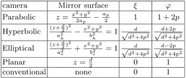
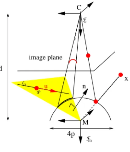
As noted previously, a single center of projection is a desirable property for an imaging system. A single center implies that all lines passing through a 3D point and its projection in the image plane pass through a single point in 3D space. Conventional perspective cameras are single view point sensors. As shown in [2], a central catadioptric system can be built by combining an hyperbolic, elliptical or planar mirror with a perspective camera and a parabolic mirror with an orthographic camera. To simplify notations conventional perspective cameras will be embedded in the set of central catadioptric cameras. In [12], a unifying theory for central panoramic systems is presented. According to this generic model, all central panoramic cameras can be modeled by a central projection onto a sphere followed by a central projection onto the image plane (see Fig. 1). This generic model can be parametrized by the couple (ξ, ϕ) (see Tab.1 and refer to [4]).
camera Mirror surface ξ ϕ
Parabolic z=x2+y2 2ap − ap 2 1 1 + 2p Hyperbolic (z+d2)2 a2 h − x2+y2 b2 h = 1 √ d d2+4p2 d+2p √ d2+4p2 Elliptical (z+d2)2 a2 e + x2+y2 b2 e = 1 d √ d2+4p2 d−2p √ d2+4p2 Planar z= d 2 0 1 conventional none 0 1
Table 1.Central catadioptric cameras description:
ap, ah, bh, ae, bedepend only of the mirror intrinsic parameters d and p
Let Fcand Fmbe the frames attached to the conventional camera and to the
mirror respectively. In the sequel, we suppose that Fc and Fmare related by a
translation along the Z-axis. The centers C and M of Fc and Fmwill be termed
optical center and principal projection center respectively. Let X be a 3D point
with coordinates X = [X Y Z]T with respect to F
m. According to the generic
projection model [12], X is projected in the image plane to a point x = [x y 1]T
with:
x= KMf (X) (1)
where K denote the triangular calibration matrix of the conventional camera, and: M= ϕ− ξ 0 0 0 ϕ− ξ 0 0 0 1 , f(X) = X Z+ξ√X2+Y2+Z2 Y Z+ξ√X2+Y2+Z2 1
In the sequel, we will assume without loss of generality that the matrices K and M are equal to the identity matrix, the mapping function describing central catadioptric projection is then given by x = f (X).
M C Fm Fc image plane P Li u d 4p x n
Fig. 1.Generic camera model
2.2 Projection of Lines
In order to model lines projection in the image of a central imaging system,
we use the Pl¨ucker coordinates of lines (refer to Fig. 1). Let P be a 3D point
and u = (ux, uy, uz)T a unit vector expressed in the mirror frame and L the
3-D line they define. Define n = −−→MP×u
k−−→MP×uk = (nx, ny, nz)
T and remark that this
vector is independent of the point we choose on the line. Thus the Euclidean
Pl¨ucker coordinates are defined as L : ¡nT uT¢T with nTu= 0. The n-vector
is orthogonal to the interpretation plane Π defined by the line and the principal projection center:
X= [X, Y, Z]T ∈ Π ⇐⇒ nxX+ nyY + nzZ= 0 (2)
Let S be the intersection between the interpretation plane and the mirror surface. S represents the line projection in the mirror surface. The projection S of L in the image is then obtained using perspective or orthographic mapping. It can be shown (using (1), (2), and the mirror surface equations given in Tab. 1, or following [3]) that 3D points lying on L are mapped into points in the image x which verify: xTΩx= 0 (3) with : Ω= Ãαn2 x− nηzξ2 αnxny βnxnη−1z αnxny αn2y− n η zξ2βnynη−1z βnxnη−1z βnynη−1z nηz !
where α = 1−ξ2, β = 2η−3, η = 2 in the general case and η = 1 for the
combina-tion parabolic mirror-orthographic camera. A line in space is thus mapped onto the image plane to a conic curve. The relation (3) defines a quadratic equation:
with: A0= sn 2 x(1−ξ 2 )−nη zξ 2 (ϕ−ξ)2 , A1= s n2 y(1−ξ 2 )−nη zξ 2 (ϕ−ξ)2 , A2= s nxny(1−ξ2) (ϕ−ξ)2 , A3= s(2η − 3)nxn η−1 z ϕ−ξ , A4= s(2η − 3) nynη−1z ϕ−ξ , A5= snηz. (5)
Let us note that the equation (4) is defined up to a scale factor s. We thus
normalize (4) using A5 to obtain unambiguous representations, the quadratic
equation is thus rewritten as follow:
B0x2+ B1y2+ 2B2xy+ 2B3x+ 2B4y+ 1 = 0 (6)
with Bi = AA5i. The case nz = 0 corresponds to a degenerate configuration of
our representation where the optical axis lies on the interpretation plane. In the
following, we consider that nz6= 0. Let us note that the normal vector n can be
computed from (5) since knk = 1. nz= (B 2 3+B42 β + 1)−1/2= Bn nx=B3βBn ny= B4βBn (7) Since nT
u= 0, note also that uz can be rewritten as:
uz= −
B3ux+ B4uy
β (8)
3
Control law
Consider the vector s = (s1T, s2T,· · · snT)T, where si is a m-dimensional
vec-tor containing the visual observations used as input of the image-based control scheme. If the 3D features corresponding to visual observations are motionless,
the time derivative of si is:
˙ si= ∂si ∂r dr dt = JiT
where T is a 6-dimensional vector denoting the velocity of the central cata-dioptric camera and containing the instantaneous angular velocity ω and the instantaneous linear velocity v of a given point expressed in the mirror frame.
The m × 6 matrix Ji is the interaction matrix (or image Jacobian). It links the
variation of the visual observations to the camera velocity. If we consider the
time derivative of s, the corresponding interaction matrix is J = (Ji,· · · , Jn)T
and ˙s = JT. To design an image-based control law, we use the task function ap-proach introduced by Samson et al in [19]. Consider the following task function
eto be regulated to 0:
where s∗ is the desired value of the observation vector s and bJ+ is the
pseudo-inverse of a chosen model of J. The time derivative of the task function is:
˙e = dbJ
+
dt (s − s
∗) + bJ+˙s = (O(s − s∗) + bJ+J)T
O(s − s∗) is a 6-dimensional square matrix such that (O(s − s∗)|s=s∗ = 0 If we
consider the following control law:
T= −λe = −λbJ+(s − s∗) (9)
then the closed-loop system is ˙e = −λ(O(s − s∗) + bJ+J)e. It is well know that
such system is locally asymptotically stable in a neighbourhood of s∗if and only
if bJ+J is a positive defined matrix. In order to compute the control law (9) it
is necessary to provide an approximated interaction matrix bJ. In the sequel,
we derive from the projection model of line for central catadioptric cameras a generic analytical form of the interaction matrix.
4
Interaction matrix for conics
In this section, first we study a generic formulation for the image Jacobian of projected lines (conics) and then we derive from this generic formulation the image Jacobian for paracatadioptric cameras.
4.1 Generic Image Jacobian
Let us first define the observation vector si for a projected line (conic) in the
central catadioptric image as:
si=£B0B1B2B3B4¤
T
(10)
and the observation vector for n conics as s = (sT
1 · · · sTn)T. Note that the
obser-vation vector is minimal for a general conic and represents without ambiguities a generic planar conic since such curves are defined by 5 parameters and defined without ambiguities by equation (6). As we will see in the sequel, the observa-tion vector can be reduced for particular central catadioptric cameras such as
the parabolic one. The interaction matrix for the observation vector sn is:
Ji= ∂si ∂r = ∂si ∂ni ∂ni ∂r = JsniJni (11)
where ni = (nxi, nyi, nzi)T is the normal vector to the interpretation plane for
line Li expressed in the mirror frame, Jsni represents the interaction between
the visual observation motion and the normal vector variation, and Jnilinks the
normal variations to the camera motions. It can easily be shown that [1]:
˙ui= −ω × ui
According to the previous equations (7) and (8), the interaction between the normal vector and the camera motion is thus:
Jni= 0 B3ux+B4uy β uy 0 −Bn B4Bn β −B3ux+B4uy β 0 −ux Bn 0 −B3βBn −uy ux 0 −B4βBn B3βBn 0 (12)
The Jacobian Jsni is obtained by computing the partial derivative of (10) with
respect to ni and according to (7):
Jsni= 1 βBnη 2αB3Bn 0 −ηαβ B32Bn 0 2αB4Bn −ηαβ B42Bn αB4Bn αB3Bn −ηαβ B3B4Bn β2Bnη−1 0 −βB3Bη−1n 0 β2Bnη−1 −βB4Bη−1n (13)
The interaction matrix can finally be computed by combining the equations (12) and (13) according to relation (11). Note that the rank of the interaction matrix given by (11) is 2. At least three lines are thus necessary to control the 6 dof of a robotic arm. As previously explained, a chosen estimation of the interaction matrix is used to design the control law. The value of J at the desired position is a typical choice. In this case, the 3D parameters have to be estimated only for the desired position. In the next part, we study the particular case of paracatadioptric camera (parabolic mirror combined to orthographic camera).
4.2 A case study: paracatadioptric cameras
In the case of paracatadioptric cameras, we have ξ = 1, α = 0 and η = 1. The lines are projected onto the image plane as circles or ellipses if the pixels
are not square. It can be noticed that A2 = 0 and A0 = A1 = −A5 and thus
the observation vector can be reduced as si = [B3B4]T. Note also that if the
pixels are square a line is projected as circle of center x = B3, y = B4 and
radius B2
3+ B42− 1. Minimizing the task function e can thus be interpreted as
minimizing the distance between current and desired centers of circles by moving
the camera. According to equation (13), the Jacobian Jsni can be reduced as
follow: Jsni= 1 Bn µ β 0 −B3 0 β −B4 
and by combining the previous relation with equation (12), the image Jacobian can be written:
J= 1
Bn
Ã
−uyB3−uyB4−uyβ −B3Bβ4Bn βBn+B
2 3Bn β −B4Bn uxB3 uxB4 uxβ −βBn−B 2 4Bn β B3B4Bn β B3Bn !
The rank of the image Jacobian is 2. Its kernel is spanned by the basis composed of the vectors:
(0, 1,B4β ,0, 0, 0) (0, 0, −B4Bn(B 2 3+B2+B24) β2(uy B3−uxB4) ,1, 0,
(uy B3+uy B24β+uxB23B4uy −u2x B3 B42)
β ) (1, 0, −B3β ,0, 0, 0) (0, 0,B3Bn(β4+B23β2+B24uy B3−B 3 4ux) β2 ,0, 1, −
uxB23+uy B3B4+uxB2 β(uy B3−uxB4) )
The six degrees of freedom of a robotic arm can thus be fully controlled using three projected lines as long as the lines define three different interpretations planes.
5
Simulation results
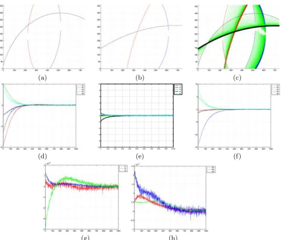
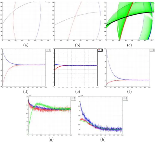
In this section, we present simulation results of central catadioptric visual ser-voing from lines by using the control law (9). The value of J at the desired position has been used. We have considered two positioning tasks. From an ini-tial position, the robot has to reach a desired position expressed as a desired observation vector. The first simulation concerns a camera combining an hyper-bolic mirror and a perspective camera (Fig. 3). The second simulation concerns a camera combining a parabolic mirror and an orthographic camera (Fig. 4). The initial attitude of the camera with respect to the world frame is given by
ri = [0, 0, 1, 0, 0, 0]T (the first three components are the translations in
meter and the last three are the rotations in radian). The desired image
corre-sponds to the camera configuration given by rd= [0.1, 0.1, 1.1, π8, π8, π8]T in
the world frame. The three lines are defined in the world space by the following
Pl¨ucker coordinates: L1: µ u1= (0 1 0)T n1= (0 0 − 1)T ¶ L2: µ u2= (0 0.9806 0.1961)T n2= (0 − 0.1961 0.9806)T ¶ L3: µ u3= (0.9623 0.1925 0.1925)T n3= (0.1961 0 − 0.9806)T 
Figure 2 shows the initial spatial configurations of lines and camera. Image noise has been introduced (additive noise with maximum amplitude of 1 pixel) in the
observation vectors. The Pl¨ucker coordinates of the considered lines with respect
to the world frame have been corrupted with errors of maximal amplitude of 5% (these errors corrupt the estimation of the interaction matrix at the desired configuration). The images corresponding to the initial and desired cameras po-sitions are given in Figures 3(a) and 3(b) for the hyperbolic-perspective camera 4(a) and 4(b) for the parabolic-orthographic camera. Figures 3(c) and 4(c) shows the trajectories of the conics in the image plane. Camera velocities are given in Figures 3(g), 3(h) and 4(g), 4(h). As can been seen in Figures showing the errors between desired and current observation vectors (Figs. 3(d), 3(e), 3(f) and 4(d),
4(e), 3(f)), the positioning task is correctly realized as well for the hyperbolic-perspective camera as for the parabolic-orthographic camera. Note finally, that these results confirm that visual servoing schemes can benefit from the use of central catadioptric vision systems to cope with visibility constraints.
6
Conclusions
Visibility constraints are extremely important for visual servoing applications. To overcome these constraints, the wide field of view of central catadioptric cameras can be exploited. We have addressed the problem of controlling a robotic arm by incorporating observations from a central catadioptric camera. A generic image Jacobian has been derived from the model of line projection and a control law designed. The proposed approach will be used to control a six degrees of freedom manipulator. Future work will be devoted to study the case of nonholonomic robots and path planning in central catadioptric image space.
Acknowledgment
This work has been funded by the project OMNIBOT of ROBEA:”Robotique et Entit´es Artificielles”.
References
1. N. Andreff, B. Espiau, and R. Horaud. Visual servoing from lines. International Journal of Robotics Research, 21(8):679–700, August 2002.
2. S. Baker and S. K. Nayar. A theory of single-viewpoint catadioptric image forma-tion. International Journal of Computer Vision, 35(2):1–22, November 1999. 3. J. Barreto and H. Araujo. Geometric properties of central catadioptric line
im-ages. In 7th European Conference on Computer Vision, ECCV’02, pages 237–251, Copenhagen, Denmark, May 2002.
4. J. P. Barreto, F. Martin, and R. Horaud. Visual servoing/tracking using central catadioptric images. In ISER2002 - 8th International Symposium on Experimental Robotics, pages 863–869, Bombay, India, July 2002.
5. R. Benosman and S. Kang. Panoramic Vision. Springer Verlag, 2000.
6. P. Blaer and P.K. Allen. Topological mobile robot localization using fast vision techniques. In IEEE International Conference on Robotics and Automation, pages 1031–1036, Washington, USA, May 2002.
7. D. Burshka, J. Geiman, and G. Hager. Optimal landmark configuration for vision based control of mobile robot. In IEEE International Conference on Robotics and Automation, pages 3917–3922, Tapei, Taiwan, September 2003.
8. F. Chaumette. Potential problems of stability and convergence in image-based and position-based visual servoing. The Confluence of Vision and Control, D. Kriegman, G. Hager, A. Morse (eds), LNCIS Series, Springer Verlag, 237:66–78, 1998.
−2 −1.5 −1 −0.5 0 0.5 1 1.5 2 −2 −1.5 −1 −0.5 0 0.5 1 1.5 2 −2 −1.5 −1 −0.5 0 0.5 1 1.5 2 Catadioptric Camera
Fig. 2. Lines configurations in 3D
(a) (b) (c) 0 100 200 300 400 500 600 700 800 900 1000 −10 −8 −6 −4 −2 0 2 4 6 8 10 s1 s2 s3 s4 s5 (d) (e) (f) (g) (h)
Fig. 3.Hyperbolic mirror-perspective camera: (a) Initial image, (b) desired image, (c) trajectories in the image plane of line projection; Errors (s −s∗): (d) Errors for the first
conic, (e) Errors for the second conic, (f) Errors for the third conic; (g) Translational velocities [m/s] and (h) rotational velocities [rad/s]
(a) (b) (c) 0 100 200 300 400 500 600 700 800 900 1000 −25 −20 −15 −10 −5 0 5 10 15 20 s1 s2 (d) (e) (f) (g) (h)
Fig. 4.Parabolic mirror-orthographic camera: (a) Initial image , (b) desired image (c) trajectory of the catadioptric image lines; Errors (s − s∗): (d) Errors for the first conic,
(e) Errors for the second conic, (f) Errors for the third conic;(g) Translational velocities [m/s] and (h) rotational velocities [rad/s]
9. G. Chesi, K. Hashimoto, D. Prattichizzo, and A. Vicino. A switching control law for keeping features in the field of view in eye-in-hand visual servoing. In IEEE International Conference on Robotics and Automation, pages 3929–3934, Taipei, Taiwan, September 2003.
10. Noah J. Cowan, Joel D. Weingarten, and Daniel E. Koditschek. Visual servoing via navigation functions. IEEE Transactions on Robotics and Automation, 18(4):521– 533, August 2002.
11. B. Espiau, F. Chaumette, and P. Rives. A new approach to visual servoing in robotics. IEEE Transactions on Robotics and Automation, 8(3):313–326, June 1992.
12. C. Geyer and K. Daniilidis. A unifying theory for central panoramic systems and practical implications. In European Conference on Computer Vision, volume 29, pages 159–179, Dublin, Ireland, May 2000.
13. S. Hutchinson, G.D. Hager, and P.I. Corke. A tutorial on visual servo control. IEEE Transactions on Robotics and Automation, 12(5):651–670, October 1996. 14. E. Malis, J. Borrelly, and P. Rives. Intrinsics-free visual servoing with respect
to straight lines. In IEEE/RSJ International Conference on Intelligent Robots Systems, Lausanne, Switzerland, October 2002.
15. E. Malis, F. Chaumette, and S. Boudet. 2 1/2 d visual servoing. IEEE Transactions on Robotics and Automation, 15(2):238–250, April 1999.
16. Y. Mezouar and F. Chaumette. Path planning for robust image-based control. IEEE Transactions on Robotics and Automation, 18(4):534–549, August 2002. 17. A. Paulino and H. Araujo. Multiple robots in geometric formation: Control
struc-ture and sensing. In International Symposium on Intelligent Robotic Systems, pages 103–112, University of Reading, UK, July 2000.
18. E. Malis S. Benhimane. Vision-based control with respect to planar and non-planar objects using a zooming camera. In IEEE International Conference on Advanced Robotics, pages 863–869, July 2003.
19. C. Samson, B. Espiau, and M. Le Borgne. Robot Control : The Task Function Approach. Oxford University Press, 1991.
20. B. Thuilot, P. Martinet, L. Cordesses, and J. Gallice. Position-based visual servo-ing: keeping the object in the field of vision. In IEEE International Conference on Robotics and Automation, pages 1624–1629, Washington DC, USA, May 2002. 21. R. Vidal, O. Shakernia, and S. Sastry. Formation control of nonholonomic mobile
robots with omnidirectional visual servoing and motion segmentation. In IEEE International Conference on Robotics and Automation, Taipei, Taiwan, September 2003.
22. N. Winter, J. Gaspar, G. Lacey, and J. Santos-Victor. Omnidirectional vision for robot navigation. In Proc. IEEE Workshop on Omnidirectional Vision, OMNIVIS, pages 21–28, South Carolina, USA, June 2000.