Sensitivity Analysis of the Orthoglide, a 3-DOF Translational Parallel Kinematic Machine

HAL Id: hal-00170102

https://hal.archives-ouvertes.fr/hal-00170102

Submitted on 4 May 2018

HAL is a multi-disciplinary open access

archive for the deposit and dissemination of

sci-entific research documents, whether they are

pub-lished or not. The documents may come from

teaching and research institutions in France or

abroad, or from public or private research centers.

L’archive ouverte pluridisciplinaire HAL, est

destinée au dépôt et à la diffusion de documents

scientifiques de niveau recherche, publiés ou non,

émanant des établissements d’enseignement et de

recherche français ou étrangers, des laboratoires

publics ou privés.

Sensitivity Analysis of the Orthoglide, a 3-DOF

Translational Parallel Kinematic Machine

Stéphane Caro, Philippe Wenger, Fouad Bennis, Damien Chablat

To cite this version:

Stéphane Caro, Philippe Wenger, Fouad Bennis, Damien Chablat. Sensitivity Analysis of the

Or-thoglide, a 3-DOF Translational Parallel Kinematic Machine. ASME Design Engineering Technical

Conferences, Sep 2004, Salt Lake City, United States. pp.1-10, �10.1115/1.2166852�. �hal-00170102�

Institut de Recherche en Communications et Cybernétique de Nantes (IRCCyN) UMR 6597 CNRS, École Centrale de Nantes, Université de Nantes, École des Mines de Nantes 1, rue de la Noë-44321 Nantes, France

Sensitivity Analysis of the

Orthoglide: A Three-DOF

Translational Parallel Kinematic

Machine

In this paper, two complementary methods are introduced to analyze the sensitivity of a three-degree-of-freedom (3-DOF) translational parallel kinematic machine (PKM) with orthogonal linear joints: the Orthoglide. Although these methods are applied to a par-ticular PKM, they can be readily applied to 3-DOF Delta-Linear PKM such as ones with their linear joints parallel instead of orthogonal. On the one hand, a linkage kinematic analysis method is proposed to have a rough idea of the influence of the length variations of the manipulator on the location of its end-effector. On the other hand, a differential vector method is used to study the influence of the length and angular variations in the parts of the manipulator on the position and orientation of its end-effector. Besides, this method takes into account the variations in the parallelograms. It turns out that varia-tions in the design parameters of the same type from one leg to another have the same effect on the position of the end-effector. Moreover, the sensitivity of its pose to geometric variations is a minimum in the kinematic isotropic configuration of the manipulator. On the contrary, this sensitivity approaches its maximum close to the kinematic singular configurations of the manipulator.

Keywords: parallel kinematic machine, sensitivity analysis, kinematic analysis, kinematic singularity, isotropy

1 Introduction

For two decades, parallel manipulators have attracted the atten-tion of more and more researchers who consider them as valuable alternative design for robotic mechanisms. As stated by numerous authors, conventional serial kinematic machines have already reached their dynamic performance limits, which are bounded by high stiffness of the machine components required to support se-quential joints, links, and actuators. Thus, while having good op-erating characteristics共large workspace, high flexibility and ma-neuverability兲, serial manipulators have disadvantages of low stiffness and low power. Conversely, parallel kinematic machines 共PKMs兲 offer essential advantages over their serial counterparts 共lower moving masses, higher stiffness and payload-to-weight ra-tio, higher natural frequencies, better accuracy, simpler modular mechanical construction, possibility to locate actuators on the fixed base兲.

However, PKMs are not necessarily more accurate than their serial counterparts. Indeed, even if the dimensional variations can be compensated with PKM, they can also be amplified contrary to with their serial counterparts关1兴. Wang and Masory 关2兴 studied the effect of manufacturing tolerances on the accuracy of a Stew-art platform. Kim and Choi关3兴 used a forward error bound analy-sis to find the error bound of the end-effector of a Stewart plat-form when the error bounds of the joints are given, and an inverse error bound analysis to determine those of the joints for the given error bound of the end-effector. Kim and Tsai 关4兴 studied the effect of misalignment of linear actuators of a 3-DOF translational parallel manipulator on the motion of its moving platform. Han et al.关5兴 used a kinematic sensitivity analysis method to explain the gross motions of a 3-UPU parallel mechanism, and they showed

that it is highly sensitive to certain minute clearances. Fan et al. 关6兴 analyzed the sensitivity of the 3-PRS parallel kinematic spindle platform of a serial-parallel machine tool. Verner et al.关7兴 presented a new method for optimal calibration of PKM based on the exploitation of the least error sensitive regions in their work-space and geometric parameters work-space. As a matter of fact, they used a Monte Carlo simulation to determine and map the sensi-tivities to geometric parameters. Moreover, Caro et al.关8兴 devel-oped a tolerance synthesis method for mechanisms based on a robust design approach.

This paper aims at analyzing the sensitivity of the Orthoglide to its dimensional and angular variations. The Orthoglide is a 3-DOF translational PKM developed by Chablat and Wenger关9兴. A small-scale prototype of this manipulator was built at IRCCyN.

Here, the sensitivity of the Orthoglide is studied by means of two complementary methods. First, a linkage kinematic analysis is used to have a rough idea of the influence of the dimensional variations to its end-effector and to show that the variations in design parameters of the same type from one leg to another have the same influence on the location of the end-effector. Although this method is compact, it cannot be used to know the influence of the variations in the parallelograms. Thus, a differential vector method is developed to study the influence of the dimensional and angular variations in the parts of the manipulator, and particularly variations in the parallelograms, on the position and the orienta-tion of its end-effector.

In the isotropic kinematic configuration, the end-effector of the manipulator is located at the intersection between the directions of its three actuated prismatic joints, and the condition number of its kinematic Jacobian matrix is equal to 1关10兴. It is shown that this configuration is the least sensitive one to geometrical variations, contrary to the closest configurations to its kinematic singular configurations, which are the most sensitive to geometrical variations.

Although the two sensitivity analysis methods are applied to a

Stéphane Caro

Philippe Wnger

Fouad Bennis

Damien Chablat

particular PKM, these methods can be readily applied to other 3-DOF Delta-linear PKM such as ones with parallel linear joints instead of orthogonal ones.

2 Manipulator Geometry

The kinematic architecture of the Orthoglide is shown in Fig. 1. It consists of three identical parallel chains that are formally de-scribed as PRPaRR, where P, R, and Pa denote the prismatic,

revolute, and parallelogram joints, respectively, as shown in Fig. 2.

The mechanism input is made up of three actuated orthogonal prismatic joints. The output body共with a tool mounting flange兲 is connected to the prismatic joints through a set of three kinematic chains. Inside each chain, one parallelogram is used and oriented in a manner that the output body is restricted to translational movements only.

The small-scale prototype of the Orthoglide was designed to reach Cartesian velocity of 1.2 m / s and an acceleration of 17 m / s2_{. The desired payload is 4 kg 共spindle, tool, included兲.}

The size of its prescribed cubic workspace Cu is 200⫻200

⫻200 mm, where the velocity transmission factors are bounded between 1 / 2 and 2. The three legs are supposed to be identical. According to 关9兴, the nominal lengths Li and widths di of the

parallelograms, and the nominal distances, ri, between points Ci

and the end-effector P are identical, i.e., L = L₁= L₂= L₃ = 310.58 mm, d = d1= d2= d3= 80 mm, r = r1= r2= r3= 31 mm.

As depicted in Fig. 3, Q₁and Q₂, vertices of C_u, are defined at the intersection between the Cartesian workspace boundary and the axis x = y = z expressed in the reference coordinate frameRb.

Q1and Q2are the closest points to the singularity surfaces. Their

Cartesian coordinates, expressed in R_b, are equal to 共−73.21, −73.21, −73.21兲 and 共126.79, 126.79, 126.79兲, respectively.

The parts of the manipulator are supposed to be rigid bodies and there is no joint clearance. The legs of the manipulator, com-posed of one prismatic joint, one parallelogram, and three revolute joints, generate a five-DOF motion each. Besides, they are

iden-tical. Therefore, according to Karouia et al.关11兴, the manipulator is isostatic. Thus, the results obtained by the sensitivity analysis methods developed in this paper are meaningful.

3 Sensitivity Analysis

Two complementary methods are used to study the sensitivity of the Orthoglide. First, a linkage kinematic analysis is used to have a rough idea of the influence of the dimensional variations to its end-effector. Although this method is compact, it cannot be used to know the influence of the variations in the parallelograms. Thus, a differential vector method is used to study the influence of the dimensional and angular variations in the parts of the manipu-lator, and particularly variations in the parallelograms, on the po-sition and the orientation of its end-effector.

3.1 Linkage Kinematic Analysis. This method aims at

com-puting the sensitivity coefficients of the position of the end-effector, P, to the design parameters of the manipulator. First, three implicit functions depicting the kinematic of the manipulator are obtained. A relation between the variations in the position of P and the variations in the design parameters follows from these functions. Finally a sensitivity matrix, which gathers the sensitiv-ity coefficients of P, follows from the previous relation written in matrix form.

3.1.1 Formulation. Figure 1 depicts the design parameters taken into account. Points A1, A2, and A3 are the bases of the

prismatic joints. Their Cartesian coordinates, expressed inRb, are

a1, a2, and a3, respectively.

a₁=关− a₁0 0兴T _共1a兲

a₂=关0 − a₂0兴T _共1b兲

a3=关0 0 − a3兴T 共1c兲

where a_iis the distance between points A_iand O, the origin ofR_b. Points B1, B2, and B3 are the links between the prismatic and

parallelogram joints. Their Cartesian coordinates, expressed inR_b are b₁=

冤

− a1+␳1 b_1y b_1z

冥

共2a兲 b₂=

冤

b2x − a₂+␳₂ b_2z

冥

共2b兲

Fig. 1 Basic kinematic architecture of the Orthoglide

Fig. 2 Morphology of the ith leg of the Orthoglide

b₃=

冤

b_3x b3y

− a₃+␳₃

冥

共2c兲 where␳iis the displacement of the ith prismatic joint. b1yand b1z

are the position errors of point B1according to y and z axes. b2x

and b_2zare the position errors of point B₂according to the x and z axes. b3xand b3yare the position errors of point B3according to

x and y axes. These errors result from the orientation errors of the directions of the prismatic actuated joints. The Cartesian coordi-nates of C₁, C₂, and C₃, expressed inR_b, are the following:

c₁=关px− r10 0兴T 共3a兲 c2=关0 py− r20兴T 共3b兲

c₃=关0 0 pz− r3兴T 共3c兲

where p =关pxpypz兴Tis the vector of the Cartesian coordinates of

the end-effector P, expressed inRb.

The expressions of the nominal lengths of the parallelograms follow from Eq.共4兲,

Li=储ci− bi储2, i = 1,2,3 共4兲

where Liis the nominal length of the ith parallelogram and储·储2is

the Euclidean norm. Three implicit functions follow from Eq.共4兲 and are given by the following equations:

F₁=共− r₁+ px+ a1−␳1兲2+共py− b1y兲2+共pz− b1z兲2− L12= 0

F₂=共px− b2x兲2+共− r2+ py+ a2−␳2兲2+共pz− b2x兲2− L22= 0

F₃=共px− b3x兲 + 共py− b3y兲2+共− r3+ pz+ a3−␳3兲2− L32= 0

By differentiating functions F1, F2, and F3 with respect to the

design parameters of the manipulator and the position of the end-effector, we obtain a relation between the positioning error of the end-effector␦p, and the variations in the design parameters␦q_i.

␦Fi= Ai␦p + Bi␦qi= 0, i = 1,2,3 共5兲 with Ai=关⳵Fi/⳵px⳵Fi/⳵py⳵Fi/⳵pz兴 共6兲 Bi=关⳵Fi/⳵ai⳵Fi/⳵biy⳵Fi/⳵biz⳵Fi/⳵␳i⳵Fi/⳵Li⳵Fi/⳵ri兴 共7兲 ␦p =关␦px␦py␦pz兴 T 共8兲 ␦qi=关␦ai␦hi␦ki␦␳i␦Li␦ri兴T 共9兲

where␦ai,␦hi,␦ki,␦␳i,␦Li, and␦ri, depict the variations in ai, hi,

k_i, ␳_i, L_i, and r_i, respectively, with h₁= b_1y, k₁= b_1z, h₂= b_2x, k₂ = b2z, h3= b3x, k3= b3y.

Integrating the three loops of Eq. 共5兲 together and separating the position parameters and design parameters to different sides yields the following simplified matrix form:

A␦p + B␦q = 0 共10兲 with A =关A₁TA₂TA₃T兴T苸 R3⫻3 共11兲 B =

冤

B1 0 0 0 B₂ 0 0 0 B3

冥

苸 R3⫻18 _共12兲 ␦q =关␦q₁T␦qT₂␦q₃T兴T_{苸 R}18⫻1 _共13兲

Equation共10兲 takes into account the coupling effect of the three independent structure loops. According to 关9兴, A is the parallel Jacobian kinematic matrix of the Orthoglide, which does not meet parallel kinematic singularities when its end-effector covers Cu.

Therefore, A is not singular and its inverse A−1_{exists. Thus, the}

positioning error of the end-effector can be computed using Eq. 共14兲. ␦p = C␦q 共14兲 where C = − A−1B =

冤

⳵px/⳵a1 ⳵px/⳵h1 ¯ ⳵px/⳵r3 ⳵py/⳵a1 ⳵py/⳵h1 ¯ ⳵py/⳵r3 ⳵pz/⳵a1 ⳵pz/⳵h1 ¯ ⳵pz/⳵r3

冥

苸 R3⫻18 共15兲 represents the sensitivity matrix of the manipulator. The terms of

C are the sensitivity coefficients of the Cartesian coordinates of

the end-effector to the design parameters and are used to analyze the sensitivity of the Orthoglide.

3.1.2 Results of the Linkage Kinematic Analysis. The sensitiv-ity matrix C of the manipulator depends on the position of its end-effector.

Figures 4–7 depict the mean of the sensitivity coefficients of px,

py, pz, and p, when the end-effector covers Cu. It appears that the

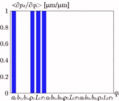
Fig. 4 Mean of sensitivity of p_xthroughout C_u Fig. 5 Mean of sensitivity of pythroughout Cu

position of the end-effector is very sensitive to variations in the position of points Ai, variations in the lengths of the

parallelo-grams, L_i, variations in the lengths of prismatic joints, ␳_i, and variations in the position of points Cidefined by ri共see Fig. 2兲.

However, it is little sensitive to the orientation errors of the direc-tion of the prismatic joints, defined by parameters b1y, b1z, b2x,

b_2z, b_3x, b_3y. Besides, it is noteworthy that p_x共p_y, p_z, respectively兲 is very sensitive to the design parameters which make up the 1st 共2nd, 3rd, respectively兲 leg of the manipulator, contrary to the others. That is due to the symmetry of the architecture of the manipulator. Henceforth, only the variations in the design param-eters of the first leg of the manipulator will be taken into account. Indeed, the sensitivity of the position of the end-effector to the variations in the design parameters of the second and the third legs of the manipulator can be deduced from the sensitivity of the position of the end-effector to variations in the design parameters of the first leg.

Chablat and Wenger关9兴 showed that if the prescribed bounds of the velocity transmission factors 共the kinematic criteria used to dimension the manipulator兲 are satisfied at Q₁and Q₂, then these bounds are satisfied throughout the prescribed cubic Cartesian workspace Cu. Q1and Q2are then the most critical points of Cu,

whereas O is the most interesting point because it corresponds to the isotropic kinematic configuration of the manipulator. Here, we assume that if the prescribed bounds of the sensitivity coefficients are satisfied at Q₁and Q₂, then these bounds are satisfied through-out Cu.

Figures 8 and 9 depict the sensitivity coefficients of p_xand p_yto the dimensional variations in the 1st leg, i.e., a1, b1y, b1z,␳1, L1,

r1, along Q1Q2. It appears that these coefficients are a minimum in

the isotropic configuration, i.e., P⬅O, and a maximum when P ⬅Q2, i.e., in the closest configuration to the singular one. Figure

10 depicts the sensitivity coefficients of p along diagonal Q₁Q₂. It is noteworthy that all the sensitivity coefficients are a minimum when P⬅O and a maximum when P⬅Q2. Finally, Fig. 11 depicts

the global sensitivities of p, px, py, and pz to the dimensional

variations. It appears that they are a minimum when P⬅O, and a

maximum when P⬅Q₂.

Figures 12 and 13 depict the sensitivity coefficients of pxand p

in the isotropic configuration. In this configuration, the position error of the end-effector does not depend on the orientation errors of the directions of the prismatic joints because the sensitivity of the position of P to variations in b_1y, b_1z, b_2x, b_2z, b_3x, b_3yis null in this configuration. Besides, variations in p_x, p_y, and p_zare de-coupled in this configuration. Indeed, variations in px, 共py, pz,

respectively兲 are only due to dimensional variations in the 1st, 共2nd, 3rd, respectively兲 leg of the manipulator. The corresponding sensitivity coefficients are equal to 1. It means that the dimen-sional variations are neither amplified nor compensated in the iso-tropic configuration.

Figures 14 and 15 depict the sensitivity coefficients of p_xand p when the end-effector hits Q2共P⬅Q2兲. In this case, variations in

px, py, and pzare coupled. For example, variations in pxare due to

both dimensional variations in the 1st leg and variations in the 2nd and the 3rd legs. Besides, the amplification of the dimensional variations is important. Indeed, the sensitivity coefficients of p are close to 2 in this configuration. For example, as the sensitivity

Fig. 7 Mean of sensitivity of p throughout Cu

Fig. 9 Sensitivity of pyto the variations in the 1st leg

Fig. 10 Sensitivity of p to the variations in the 1st leg

Fig. 11 Global sensitivity of p, p_x, p_y, and p_z Fig. 8 Sensitivity of p_xto the variations in the 1st leg

coefficient relating to L1is equal to 1.9, the position error of the

end-effector will be equal to 19␮m if␦L₁= 10␮m. Moreover, we noticed numerically that Q2 configuration is the most sensitive

configuration to dimensional variations of the manipulator.

According to Figs. 4–7 and 12–15, variations in design param-eters of the same type from one leg to another have the same influence on the location of the end-effector.

However, this linkage kinematic method does not take into ac-count variations in the parallelograms, except the variations in their global length. Thus, a differential vector method is devel-oped below.

3.2 Differential Vector Method. In this section, we perfect a

sensitivity analysis method of the Orthoglide, which complements the previous one. This method is used to analyze the sensitivity of the position and the orientation of the end-effector to dimensional and angular variations, and particularly to the variations in the parallelograms. Moreover, it allows us to distinguish the varia-tions which are responsible for the position errors of the end-effector from the ones which are responsible for its orientation errors. To develop this method, we were inspired by a Huang & al. work on a parallel kinematic machine, which is made up of par-allelogram joints too关12兴.

First, we express the dimensional and angular variations in vec-torial form. A relation between the position and the orientation errors of the end-effector is then obtained from the closed-loop kinematic equations. The expressions of the orientation and the position errors of the end-effector, with respect to the variations in the design parameters, are deduced from this relation. Finally, we introduce two sensitivity indices to assess the sensitivity of the position and the orientation of the end-effector to dimensional and angular variations, and particularly to the parallelism errors of the bars of the parallelograms.

3.2.1 Formulation. The schematic drawing of the ith leg of the Orthoglide depicted in Fig. 2 is split in order to depict the variations in design parameters in a vectorial form. The closed-loop kinematic chains O − Ai− Bi− Bij− Cij− Ci− P, i = 1 , 2 , 3, j

= 1 , 2, are depicted by Figs. 16–19.Ri is the coordinate frame

attached to the ith prismatic joint. o, a_i, b_i, b_ij, c_ij, c_i, p, are the Cartesian coordinates of points O, Ai, Bi, Bij, Cij, Ci, P,

respec-tively, expressed inRiand depicted in Fig. 2.

According to Fig. 16,

Fig. 12 Sensitivity of pxin the isotropic configuration

Fig. 13 Sensitivity of p in the isotropic configuration

Fig. 14 Q2configuration, sensitivity of px

Fig. 16 Variations in O − Aichain

Fig. 17 Variations in A_i− B_ichain Fig. 15 Q₂ configuration, sensitivity of p

ai− o = Ri共a0+␦ai兲 共16兲

where a0is the nominal position vector of Aiwith respect to O

expressed inR_i,␦a_iis the positioning error of A_i. R_iis the trans-formation matrix fromRitoRb. I3is the共3⫻3兲 identity matrix

and R1= I3 共17兲 R2=

冤

0 0 − 1 1 0 0 0 − 1 0

冥

共18兲 R₃=

冤

0 1 0 0 0 1 1 0 0

冥

共19兲 According to Fig. 17, bi− ai= Ri共␳i+␦␳i兲e1+ Ri␦␪Ai⫻ 共␳i+␦␳i兲e1 共20兲

where␳_iis the displacement of the ith prismatic joint,␦␳_iis its displacement error,␦␪_Ai=关␦␪_Aix␦␪_Aiy␦␪_Aiz兴T_{is the angular}

varia-tion of its direcvaria-tion, and

e₁=

冤

1 0 0

冥

共21兲 e₂=

冤

0 0 1

冥

共22兲 ␰共j兲 =

再

1, if j = 1 − 1, if j = 2

冎

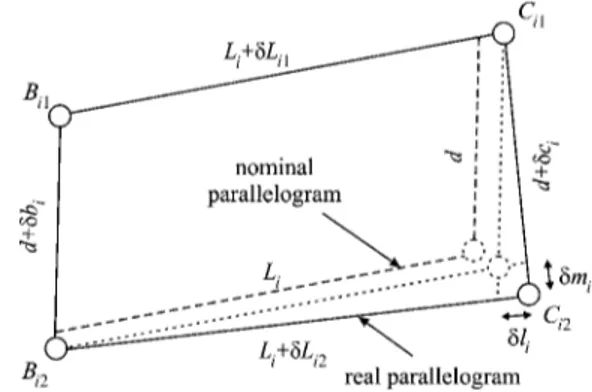
共23兲 According to Fig. 18,

bij− bi= Ri关I3+␦␪Ai⫻ 兴共␰共j兲共d/2 +␦bi/2兲关I3+␦␪Bi⫻ 兴e2兲

共24兲

cij− bij= Liwi+␦Liwi+ Li␦wi 共25兲

where d is the nominal width of the parallelogram, ␦b_i is the variation in the length of link B_i1B_i2and is supposed to be equally shared by each side of Bi.␦␪Bi=关␦␪Bix␦␪Biy␦␪Biz兴Tis the

orien-tation error of link Bi1Bi2with respect to the direction of the ith

prismatic joint, L_iis the length of the ith parallelogram,␦L_ijis the variation in the length of link B_ijC_ij, of which w_iis the direction, and␦wiis the variation in this direction, orthogonal to wi.

According to Fig. 19,

cij− ci= Ri关I3+␦␪ ⫻ 兴共␰共j兲共d/2 +␦ci/2兲关I3+␦␪Ci⫻ 兴e2兲

共26兲

ci− p =关I3+␦␪ ⫻ 兴Ri共c0+␦ci兲 共27兲

where␦c_i is the variation in the length of link C_i1C_i2, which is supposed to be equally shared by each side of Ci.

␦␪Ci=关␦␪Cix␦␪Ciy␦␪Ciz兴T is the orientation error of link Ci1Ci2

with respect to link CiP. c0is the nominal position vector of Ci

with respect to end-effector P, expressed inR_i,␦c_iis the position error of Ciexpressed inRi, and␦␪=关␦␪x␦␪y␦␪z兴T is the

orien-tation error of the end-effector, expressed inRb.

Implementing linearization of Eqs.共16兲–共26兲 and removing the components associated with the nominal constrained equation p0

= R_i共a₀+␳_ie₁− c₀兲+L_iw_i, yields

␦p = p − p₀= Ri共␦ei+␳i共␦␪Ai⫻ e1兲 +␰共j兲d/2共␦␪Ai⫻ e2兲

+␰共j兲d/2共␦␥i⫻ e2兲 +␰共j兲␦mi/2e2兲 +␦Lijwi+ Li␦wi−␦␪

⫻ Ri共c0+ d/2␰共j兲e2兲 共28兲

where␦p is the position error of the end-effector of the

manipu-lator; ␦ei=␦ai+␦␳ie1−␦ci is the sum of the position errors of

points A_i, B_i, and C_iexpressed inR_i;␦␥_i=␦␪_Bi−␦␪_Ciis the sum of the orientation errors of the ith parallelogram with respect to the ith prismatic joint and the end-effector;␦m_i=␦b_i−␦c_i corre-sponds to the parallelism error of links B_i1C_i1and B_i2C_i2, which is depicted by Fig. 20.

Equation共28兲 shows the coupling of the position and orienta-tion errors of the end-effector. Contrary to the orientaorienta-tion error, the position error can be compensated because the manipulator is a translational 3-DOF PKM. Thus, it is more important to mini-mize the geometrical variations, which are responsible for the orientation errors of the end-effector than the ones, which are responsible for its position errors.

The following equation is obtained by multiplying both sides of Eq.共28兲 by w_iTand utilizing the circularity of hybrid product.

Fig. 18 Variations in Bi− Bij− Cijchain

Fig. 20 Variations in the ith parallelogram

w_iT␦p = w_iTRi␦ei+␳i共Rie1⫻ wi兲TRi␦␪Ai+␰共j兲d/2共Rie2 ⫻ wi兲TRi共␦␪Ai+␦␥i兲 +␰共j兲␦mi/2wi T Rie2+␦Lij−兵Ri关c0 +␰共j兲d/2e₂兴 ⫻ wi其 T_␦␪ 共29兲 3.2.1.1 Orientation Error Mapping Function. By subtraction of Eqs.共29兲 written for j=1 and j=2, and for the ith kinematic chain, a relation is obtained between the orientation error of the end-effector and the variations in design parameters, which is in-dependent of the position error of the end-effector.

d共Rie2⫻ wi兲T␦␪ =␦li+ d共Rie2⫻ wi兲TRi共␦␪Ai+␦␥i兲 +␦miwi T

Rie2

共30兲 where␦l_i=␦L_i1−␦L_i2, the relative length error of links B_i1C_i1and B_i2C_i2, depicts the parallelism error of links B_i1B_i2and C_i1C_i2as shown in Fig. 20. Equation共30兲 can be written in matrix form:

␦␪ = J␪␪␧␪ 共31兲 with J_␪␪= D−1_{E 共32兲} D = d

冤

共R1e2⫻ w1兲T 共R2e2⫻ w2兲 T 共R3e2⫻ w3兲T

冥

共33兲 E =

冤

E1 ¯ ¯ ¯ E2 ¯ ¯ ¯ E3

冥

共34兲 Ei=关1 wi T Rie2d共Rie2⫻ wi兲TRid共Rie2⫻ wi兲TRi兴 共35兲

␦␪ is the orientation error of the end-effector expressed in Rb, and

␧␪=共␧␪T1,␧T␪2,␧␪T3兲Tsuch that␧␪i=共␦li,␦mi,␦␪AiT,␦␥iT兲T. The

deter-minant of D will be null if the normal vectors to the plans, which contain the three parallelograms respectively, are collinear, or if one parallelogram is flat. Here, this determinant is not null when P covers C_ubecause of the geometry of the manipulator. Therefore,

D is nonsingular and its inverse D−1exists.

As共Rie2⫻wi兲T⬜Rie2,␦␪Aiz, and␦␥iz, the third components of

␦␪Aiand␦␥iexpressed inRi, have no effect on the orientation of

the end-effector. Thus, matrix J_␪␪can be simplified by eliminating its columns associated with␦␪_Aizand␦␥_iz, i = 1 , 2 , 3. Finally, eigh-teen variations:␦l_i,␦m_i,␦␪_Aix,␦␪_Aiy,␦␥_ix,␦␥_iy, i = 1 , 2 , 3, should be responsible for the orientation error of the end-effector.

3.2.1.2 Position Error Mapping Function. By addition of Eqs. 共29兲 written for j=1 and j=2, and for the ith kinematic chain, a relation is obtained between the position error of the end-effector and the variations in design parameters, which does not depend on ␦␥i. wi T_␦ p =␦Li+ wi T Ri␦ei+␳i共Rie1⫻ wi兲TRi␦␪Ai−共Ric0⫻ wi兲T␦␪ 共36兲 Equation共36兲 can be written in matrix form:

␦p = Jpp␧p+ Jp_␪␧_␪=关JppJp_␪兴

冋

␧p ␧␪

册

共37兲 with Jpp= F−1G 共38兲 Jp␪= F−1HJ␪␪ 共39兲 F =关w₁w₂w₃兴T 共40兲 G = diag共Gi兲 共41兲 Gi=关1 wi T Ri␳i共Rie1⫻ wi兲TRi兴 共42兲 H = −关R₁c₀⫻ w₁R₂c₀⫻ w₂R₃c₀⫻ w₃兴 共43兲 ␧p=共␧p1 T ,␧_p2T,␧_p3T兲T 共44兲 ␧pi=共␦Li,␦ei T ,␦␪Ai T 兲T _共45兲

␦Li=共␦Li1+␦Li2兲/2 is the mean value of the variations in links

Bi1Ci1and Bi2Ci2, i.e., the variation in the length of the ith

paral-lelogram. ␧_p is the set of the variations in design parameters, which should be responsible for the position errors of the end-effector, except the ones which should be responsible for its ori-entation errors, i.e.,␧_␪.␧pis made up of three kinds of errors: the

variation in the length of the ith parallelogram 共i.e., ␦L_i, i = 1 , 2 , 3兲, the position errors of points A_i, B_i, and C_i, 共i.e.,␦e_i, i = 1 , 2 , 3兲 and the orientation errors of the directions of the pris-matic joints共i.e.,␦␪_Ai, i = 1 , 2 , 3兲. Besides, F is nonsingular and its inverse F−1 exists because F corresponds to the Jacobian kine-matic matrix of the manipulator, which is not singular when P covers C_u,关9兴.

According to Eq. 共36兲 and as 共Rie1⫻wi兲T⬜Rie1, matrix Jpp

can be simplified by eliminating its columns associated with␦␪_Aix, i = 1 , 2 , 3. Finally, 33 variations:␦Li,␦eix,␦eiy,␦eiz,␦␪Aix,␦␪Aiy,

␦␪Aiz,␦li,␦mi,␦␥ix,␦␥iy, i = 1 , 2 , 3, should be responsible for the

position error of the end-effector.

Rearranging matrices J_ppand J_p␪, the position error of the end-effector can be expressed as:

␦p = J␧q=关J1J2J3兴共␧q1␧q2␧q3兲T 共46兲

with ␧_qi=共␦L_i,␦e_ix,␦e_iy,␦e_iz,␦␪_Aix,␦␪_Aiy,␦␪_Aiz,␦l_i,␦m_i, ␦␥ix,␦␥iy兲, and J苸R3⫻33.

3.2.1.3 Sensitivity Indices. In order to investigate the influence of the design parameters errors on the position and the orientation of the end-effector, sensitivity indices are required. According to Sec. 3.1.2, variations in the design parameters of the same type from one leg to the other have the same influence on the location of the end-effector. Thus, assuming that variations in the design parameters are independent, the sensitivity of the position of the end-effector to the variations in the kth design parameter respon-sible for its position error, i.e.,␧_{q共1,2,3兲k}, is called␮_kand is defined by Eq.共47兲. ␮k=

冑

兺

i=1 3

兺

m=1 3 Jimk 2 , k = 1, . . . ,11 共47兲 Likewise,␯_ris a sensitivity index of the orientation of the end-effector to the variations in the rth design parameter responsible for its orientation error, i.e.,␧_{␪共1,2,3兲r}. ␯rfollows from; Eq. 共31兲

and is defined by Eq.共48兲. ␯r= arccos

tr共Qr兲 − 1

2 共48兲

where Q_ris the rotation matrix corresponding to the orientation error of the end-effector, and␯r is a linear invariant: its global

rotation关13兴. Qr=

冤

C_␯ zrC␯yr 共C␯zrS␯yrS␯xr− S␯zrC␯xr兲 共C␯zrS␯yrC␯xr+ S␯zrS␯xr兲 S_␯ zrC␯yr 共S␯zrS␯yrS␯xr+ C␯zrC␯xr兲 共S␯zrS␯yrC␯xr− C␯zrS␯xr兲 − S_␯ yr C␯yrS␯xr C␯yrC␯xr

冥

共49兲 such that C_␯

xr= cos␯xr, S␯xr= sin␯xr, C␯yr= cos␯yr, S␯yr= sin␯yr,

C_␯

zr= cos␯zr, S␯zr= sin␯zr, and

␯xr=

冑

兺

j=0

2

␯yr=

冑

兺

j=0 2 J_{␪␪2共6j+r兲}2 , r = 1, . . . ,6 共51兲 ␯zr=

冑

兺

j=0 2 J_{␪␪3共6j+r兲}2 , r = 1, . . . ,6 共52兲 Finally,␮_k can be employed as a sensitivity index of the posi-tion of the end-effector to the kth design parameter responsible for the position error. Likewise,␯rcan be employed as a sensitivity

index of the orientation of the end-effector to the rth design pa-rameter responsible for the orientation error. It is noteworthy that these sensitivity indices depend on the location of the end-effector.

3.2.2 Results of the Differential Vector Method. The sensitiv-ity indices defined by Eqs.共47兲 and 共48兲 are used to evaluate the sensitivity of the position and orientation of the end-effector to variations in design parameters, particularly to variations in the parallelograms.

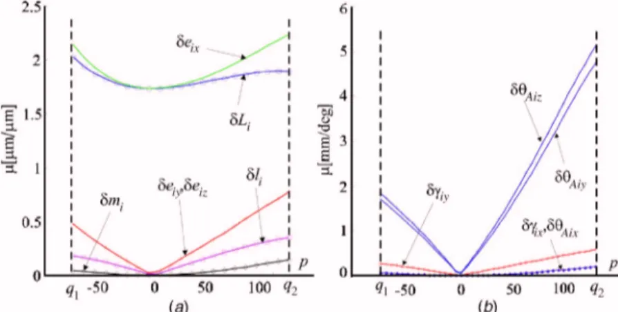
Figures 21共a兲 and 21共b兲 depict the sensitivity of the position of the end-effector along the diagonal Q₁Q₂of C_u, to dimensional variations and angular variations, respectively. According to Fig. 21共a兲, the position of the end-effector is very sensitive to varia-tions in the lengths of the parallelograms,␦Li, and to the position

errors of points A_i, B_i, and C_ialong axis x_iofR_i, i.e.,␦e_ix. Con-versely, the influence of␦liand␦mi, the parallelism errors of the

parallelograms, is low and even negligible in the kinematic iso-tropic configuration. According to Fig. 21共b兲, the orientation er-rors of the prismatic joints depicted by␦␪Aiy and ␦␪Aiz are the

most influential angular errors on the position of the end-effector. Besides, the position of the end-effector is not sensitive to angular

variations in the isotropic configuration.

Figures 22共a兲 and 22共b兲 depict the sensitivity of the orientation of the end effector, along Q₁Q₂, to dimensional and angular varia-tions. According to Fig. 22共a兲,␦l_i and ␦m_iare the only dimen-sional variations, which are responsible for the orientation error of the end-effector. However, the influence of the parallelism error of the small sides of the parallelograms, depicted by ␦l_i, is more important than the one of the parallelism error of their long sides, depicted by␦mi.

According to Figs. 21 and 22, the sensitivity of the position and the orientation of the end-effector is generally null in the kine-matic isotropic configuration共p=0兲, and is a maximum when the manipulator is close to a kinematic singular configuration, i.e., P⬅Q2. Indeed, only two kinds of design parameters variations

are responsible for the variations in the position of the end-effector in the isotropic configuration:␦L_iand␦e_ix. Likewise, two kinds of variations are responsible for the variations in its orien-tation in this configuration:␦l_i, the parallelism error of the small sides of the parallelograms,␦␪_Aiy and ␦␥_iy. Moreover, the sensi-tivities of the pose共position and orientation兲 of the end-effector to these variations are a minimum in this configuration, except for ␦li. On the contrary, Q2 configuration, i.e., P⬅Q2, is the most

sensitive configuration of the manipulator to variations in its de-sign parameters. Indeed, as depicted by Figs. 21 and 22, variations in the pose of the end-effector depend on all the design parameters variations and are a maximum in this configuration.

Moreover, Figs. 21 and 22 can be used to compute the varia-tions in the position and the orientation of the end-effector with knowledge of the amount of variations in design parameters. For instance, let us assume that the parallelism error of the small sides of the parallelograms共␦li兲, is equal to 10␮m. According to Fig.

Fig. 21 Sensitivity of the position of the end-effector along Q1Q2:„a… to

dimen-sional variations and_{„b… to angular variations}

Fig. 22 Sensitivity of the orientation of the end-effector along Q1Q2: „a… to

22共a兲, the position error of the end-effector will be equal about to 3␮m in Q₁configuration共P⬅Q₁兲. Likewise, according to Fig. 21共b兲, if the orientation error of the direction of the ith prismatic joint round axis y_iofR_iis equal to 1 deg, i.e.,␦␪_Aiy= 1 deg, the position error of the end-effector will be equal about to 4.8 mm in Q2configuration.

Let us assume now that the length and angular tolerances are equal to 0.05 mm and 0.03 deg, respectively. Figure 23共a兲 shows the maximum position error of the end-effector when it follows diagonal Q1Q2of cube Cu. Likewise, Fig. 23共b兲 shows the

maxi-mum orientation error of the end effector along Q1Q2. On both

sides, the error is a minimum when the manipulator is in its kine-matic isotropic configuration and is a maximum in Q₂ configura-tion. Besides, the maximum position and orientation errors of the end-effector are equal to 0.7 mm and 0.4 deg, respectively. These values correspond to the worst case scenario, which is unlikely.

In order to take into account realistic machining tolerances, let us assume that the distribution of length and angular variations is normal.

Figures 24共a兲 and 24共b兲 illustrate the repartition of the position and the orientation errors of the end-effector in Q1configuration,

respectively.

Figures 25共a兲 and 25共b兲 illustrate the repartition of the position and the orientation errors of the end-effector in the kinematic isotropic configuration, respectively.

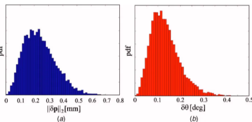
Figures 26共a兲 and 26共b兲 illustrate the repartition of the position and the orientation errors of the end-effector in Q2configuration,

respectively.

In Figures 24共a兲, 25共a兲, and 26共a兲 共共b兲, resp.兲, the horizontal axis depicts the Euclidean norm of the position共orientation, resp.兲 error of the end-effector and the vertical axis depicts the corre-sponding probability density function. To plot these figures, we

Fig. 23 Maximum position „a… and orientation „b… errors of the end-effector along Q₁Q₂

Fig. 24 Repartition of the position error_{„a… and the orientation error „b… of the} end-effector in Q1configuration

Fig. 25 Repartition of the position error„a… and the orientation error „b… of the end-effector in the isotropic configuration

computed the position and orientation errors of the end-effector corresponding to more than 3000 sets of geometric variations fol-lowing a normal distribution. For example, we can deduce from these calculations the probabilities to get a position error lower than 0.3 mm and an orientation error lower than 0.25 deg in Q₁, the isotropic, and Q2configurations.

According to Table 1, the probability to get a position error lower than 0.3 mm is higher in the kinematic isotropic configura-tion than in Q₁and Q₂configurations. However, the probability to get an orientation error lower than 0.25 deg is the same in Q1and

the isotropic configurations, but is lower in Q2configuration.

4 Conclusions

In this paper, two complementary methods were introduced to analyze the sensitivity of a three-degree-of-freedom translational parallel kinematic machine with orthogonal linear joints: the Or-thoglide. Although these methods were applied to a particular PKM, they can be readily applied to three-DOF Delta-Linear PKM such as ones with their linear joints parallel instead of or-thogonal. Indeed, the input-output equations can be set in a very similar way since all Delta-linear PKM have identical leg kine-matics, the only difference being in the closure equations关14兴.

On the one hand, a linkage kinematic analysis method was proposed to have a rough idea of the influence of the length varia-tions of the manipulator on the location of its end-effector. On the other hand, a differential vector method was developed to study the influence of the length and angular variations in the parts of the manipulator on the position and orientation of its end-effector. This method has the advantage of taking into account the varia-tions in the parallelograms.

According to the first method, variations in design parameters of the same type from one leg to another have the same effect on the end-effector. Besides, the position of the end-effector is very sensitive to variations in the lengths of parallelograms and pris-matic joints. The second method shows that the parallelism errors of the bars of parallelograms are little influential on the position of the end-effector. Nevertheless, the orientation of the end-effector of the manipulator is more sensitive to the parallelism errors of

the small sides of the parallelograms than to the ones of their long sides. Furthermore, it turns out that the sensitivity of the pose of the end-effector of the manipulator to geometric variations is a minimum in its kinematic isotropic configuration. On the contrary, this sensitivity approaches its maximum close to the kinematic singular configurations of the manipulator.

Therefore, these results should help the designer of the Or-thoglide to synthesize its dimensional tolerances. Likewise, these methods can be applied to other Delta-Linear PKM with an aim of tolerance synthesis. Finally, the next steps in our research work are to compare the sensitivity of Delta-Linear PKM to variations in their geometric parameters, and to study the relation between the sensitivity and the stiffness of such manipulators.

Acknowledgment

This research, which is part of ROBEA-MP2 project, was sup-ported by the CNRS共National Center of Scientific Research in France兲.

Nomenclature

Rb共O,x,y,z兲 ⫽ reference coordinate frame

cen-tered at O, the intersection be-tween the directions of the three actuated prismatic joints RP共P,X,Y ,Z兲 ⫽ coordinate frame attached to the

end-effector

Ri共Ai, xi, yi, zi兲 ⫽ coordinate frame attached to the

ith prismatic joint, i = 1 , 2 , 3

p =关pxpypz兴T ⫽ vector of the Cartesian

coordi-nates of the end-effector, ex-pressed inRb

␦p =关␦px␦py␦pz兴T ⫽ position error of the end-effector,

expressed inRb

␦␪=关␦␪x␦␪y␦␪z兴T ⫽ orientation error of the

end-effector, expressed inR_b ␳i ⫽ displacement of the ith prismatic

joint

␦␳i ⫽ displacement error of the ith

pris-matic joint

L_i ⫽ theoretical length of the ith parallelogram

A_i, B_i, C_i ⫽ depicted in Fig. 1

a_{i ⫽ distance between points O and Ai} r_i ⫽ distance between points P and C_i b_1y, b_1z ⫽ position errors of point B₁along y

and z axes, respectively

b_2x, b_2z ⫽ position errors of point B₂along x and z axes, respectively

b3x, b3y ⫽ position errors of point B3along x

and y axes, respectively

Fig. 26 Repartition of the position error_{„a… and the orientation error „b… of the} end-effector in Q2configuration

Table 1 Probabilities to get a position error lower than 0.3 mm and an orientation error lower than 0.25 deg in Q1, the

isotro-pic, and Q2configurations

Configuration

Q1 Isotropic Q2

Prob共储␦p储2艋0.3 mm兲 0.8468 0.9683 0.7276

h₁ ⫽ b_1y k1 ⫽ b1z h2 ⫽ b2x k2 ⫽ b2x h₃ ⫽ b_3x k₃ ⫽ b_3y

d_i ⫽ nominal width of the ith parallelogram

␦Li ⫽ variation in the length of the ith

parallelogram

␦Lij ⫽ variation in the length of link

BijCij, j = 1 , 2共see Fig. 2兲

␦b_i ⫽ variation in the length of link B_i1B_i2

␦ci ⫽ variation in the length of link

Ci1Ci2

␦l_{i ⫽ parallelism error of links Bi1}B_i2 and C_i1C_i2

␦mi ⫽ parallelism error of links Bi1Ci1

and B_i2C_i2

w_{i ⫽ direction of links Bi1}Ci1and

Bi2Ci2

␦w_i ⫽ variation in the direction of links

B_i1C_i1and B_i2C_i2

␦ei ⫽ sum of the position errors of

points Ai, Bi, Ci

␦␪Ai=关␦␪Aix␦␪Aiy␦␪Aiz兴T ⫽ angular variation in the direction

of the ith prismatic joint ␦␪Bi=关␦␪Bix␦␪Biy␦␪Biz兴T ⫽ angular variation between Bi1Bi2

and the direction of the ith pris-matic joint

␦␪Ci=关␦␪Cix␦␪Ciy␦␪Ciz兴T ⫽ angular variation between the

end-effector and C_i1C_i2

␦␥i=关␦␥ix␦␥iy␦␥iz兴T ⫽ sum of the orientation errors of

the ith parallelogram with respect to the ith prismatic joint and the end-effector

DOF ⫽ degree of freedom PKM ⫽ parallel kinematic machine

References

关1兴 Wenger, P., Gosselin, C., and Maillé, B., 1999, “A Comparative Study of Serial and Parallel Mechanism Topologies for Machine Tool,” Int. Workshop on Par-allel Kinematic Machines, Milan, Italy, pp. 23–35.

关2兴 Wang, J., and Masory, O., 1993, “On the Accuracy of a Stewart Platform-Part I, The Effect of Manufacturing Tolerances,” Proceedings of the IEEE Interna-tional Conference on Robotics Automation, ICRA’93, Atlanta, GA, pp. 114– 120.

关3兴 Kim, H. S., and Choi, Y. J., 2000, “The Kinematic Error Bound Analysis of the Stewart Platform,” J. Rob. Syst., 17, pp. 63–73.

关4兴 Kim, H. S., and Tsai, L.-W., 2003, “Design Optimization of a Cartesian Par-allel Manipulator,” ASME J. Mech. Des., 125, pp. 43–51.

关5兴 Han, C., Kim, J., Kim, J., and Park, F. C., 2002, “Kinematic Sensitivity Analy-sis of the 3-UPU Parallel Mechanism,” Mech. Mach. Theory, 37, pp. 787– 798.

关6兴 Fan, K.-C., Wang, H., Zhao, J.-W., and Chang, T. H., 2003, “Sensitivity Analy-sis of the 3-PRS Parallel Kinematic Spindle Platform of a Serial-Parallel Ma-chine Tool,” Int. J. Mach. Tools Manuf., 43, pp. 1561–1569.

关7兴 Verner, M., Fengfeng, X., and Mechefske, C., 2005, “Optimal Calibration of Parallel Kinematic Machines,” ASME J. Mech. Des., 127, pp. 62–69. 关8兴 Caro, S., Bennis, F., and Wenger, P., 2005, “Tolerance Synthesis of

Mecha-nisms: A Robust Design Approach,” ASME J. Mech. Des., 127, pp. 86–94. 关9兴 Chablat, D., and Wenger, P., 2003, “Architecture Optimization of a 3-DOF

Parallel Mechanism for Machining Applications, The Orthoglide,” IEEE Trans. Rob. Autom., 19, pp. 403–410.

关10兴 Zanganeh, K. E., and Angeles, J., 1994, “Kinematric Isotropy and the Opti-mum Design of Parallel Manipulators,” Int. J. Robot. Res., 16共2兲, pp. 3–9. 关11兴 Karouia, M., and Herve, J. M., 2002, “A Family of Novel Orientational 3-dof

Parallel Robots,” Proceedings of the 14th CISM-IFToMM RoManSy Sympo-sium, RoMansSy 14, edited by G. Bianchi, J. C. Guinot, and Rzymkowski, Springer Verlag, Vienna, pp. 359–368.

关12兴 Huang, T., Whitehouse, D. J., and Chetwynd, D. G., 2003, “A Unified Error Model for Tolerance Design, Assembly and Error Compensation of 3-DOF Parallel Kinematic Machines With Parallelogram Sruts,” Sci. China, Ser. E: Technol. Sci., 46共5兲, pp. 515–526.

关13兴 Angeles, J., 2002, Fundamentals of Robotic Mechanical Systems, 2nd edition, Springer-Verlag, New York.

关14兴 Chablat, D., Wenger, P., Majou, F., and Merlet, J. P., 2004, “An Interval Analy-sis Based Study for the Design and the Comparison of 3-DOF Parallel Kine-matic Machines,” Piping Eng., 23共6兲, pp. 615–624.