HAL Id: hal-01451187
https://hal.archives-ouvertes.fr/hal-01451187
Submitted on 9 Sep 2020
HAL is a multi-disciplinary open access
archive for the deposit and dissemination of
sci-entific research documents, whether they are
pub-lished or not. The documents may come from
teaching and research institutions in France or
abroad, or from public or private research centers.
L’archive ouverte pluridisciplinaire HAL, est
destinée au dépôt et à la diffusion de documents
scientifiques de niveau recherche, publiés ou non,
émanant des établissements d’enseignement et de
recherche français ou étrangers, des laboratoires
publics ou privés.
An Efficient Method for Modeling the Magnetic Field
Emissions of Power Electronic Equipment From
Magnetic Near Field Measurements
Fethi Benyoubi, Lionel Pichon, Mohamed Bensetti, Yann Le Bihan, Mouloud
Feliachi
To cite this version:
Fethi Benyoubi, Lionel Pichon, Mohamed Bensetti, Yann Le Bihan, Mouloud Feliachi. An Efficient
Method for Modeling the Magnetic Field Emissions of Power Electronic Equipment From Magnetic
Near Field Measurements. IEEE Transactions on Electromagnetic Compatibility, Institute of
Elec-trical and Electronics Engineers, 2017, 59 (2), pp.609-617. �10.1109/TEMC.2016.2643167�.
�hal-01451187�
T
An Efficient Method for Modeling the Magnetic Field Emissions of Power
Electronic Equipment from Magnetic Near Field Measurements
Fethi Benyoubi, Lionel Pichon, Mohamed Bensetti, Yann Le Bihan, Mouloud Feliachi
Abstract— In this article, we present an efficient modeling of
sources of electromagnetic disturbance using the measurement, in near-field, of the magnetic field radiated from a power electronic equipment. A model based on elemental magnetic dipoles is developed for the prediction of the radiated magnetic field. This model is obtained from measurements in the near field. For the determination of the parameters of the model, an optimization procedure is combined with a matrix inversion. Unlike standard approaches, this new technique allows to find equivalent sources with a small number of dipoles in a reduced computing time. To check the efficiency of the proposed method, we perform a comparison between a classical optimization method and the new procedure. To validate this method experimentally, near field magnetic measurements are performed to find the equivalent model in case of a mono turn coil, a toroidal coil and a DC/DC converter.
Index Terms— Equivalent sources, magnetic dipoles,
magnetic field, near fields, optimization method.
I. INTRODUCTION
HE reduction of cost and design time in embedded power electronic devices requires the development of numerical electromagnetic simulations to identify the sources of radiated fields and improve the design. In order to be able to characterize the magnetic field radiated, information about the sources of disturbance is needed. A tool for the diagnosis of radiated electromagnetic compatibility (EMC) is the measurement in the near field of the magnetic field [1-7] [9-13] [17-19] [21-24]. This measurement provides information on the emission source, which disappears when the plane wave is formed (far field domain), such as the geometry of the source and the distribution of currents on the conducting surface of the device.
F. Benyoubi and M. Feliachi are with the Research Institute of Electrical Energy of Nantes Atlantique, Saint-Nazaire, 44602 FRANCE (e-mail: fethi.benyoubi@etu.univ-nantes.fr; Mouloud.Feliachi@univ-nantes.fr). L. Pichon, M. Bensetti and Y. Le Bihan are with Group of electrical engineering, Paris, Gif-sur-Yvette, 91192 FRANCE (e-mail: Lionel.Pichon @geeps.centralesupelec.fr; Mohamed.Bensetti@geeps.centralesupelec.fr; yann.Le-Bihan@ geeps.centralesupelec.fr).
From the measurement of the magnetic field, an equivalent radiation model can be built in order to obtain the same radiation than the real device under test (DUT). Such model, based on magnetic dipoles can be easily included in 3D simulation softwares in order to provide simplicity and rapidly.
Several works have been done about equivalent radiation models. In [6] [12] [19], the authors proposed a matrix inversion to find the parameters of the equivalent model. In this method, the position of the dipoles and the number of dipoles have been already defined. Therefore, only the dipoles moments are unknown. The advantage of this approach lies in the speed of calculation time since only a linear system has to be solved. However, to find an accurate model, a very large number of measurements is needed. This may take a long measurement time and involve conditioning problems regarding the matrix of the linear system.
To avoid such difficulties, the authors of [1] [15] [21-22] use an optimization algorithm to construct the equivalent model where the unknown parameters are the positions and moments. This model can be constructed by a reduced number of dipoles. Nevertheless the computing time is heavy especially when the required number of dipoles is high.
The aim of this paper is to propose a fast technique taking advantages of the two methods. First, an optimization algorithm is used to find only the positions of dipoles (reduced number of unknown parameters). Then, the moments are deduced by a matrix inversion. In addition, this method looks for the dipoles in a finite volume, which leads to find a reduced number of unknowns.
Our new technique is compared to method with standard optimization algorithm by showing its performance with regard to the computational time.
The method has been firstly validated in the case of a simple problem (a mono turn coil and a toroid coil). Using a near field bench, we realized magnetic field cartographies and applied our algorithm to construct the equivalent model. In additional, this technique has been used to construct a model of a DC/DC converter to get closer to a real application of power electronics. The IEEE FSV tool [20] is used to study the validity of the obtained radiation model.
II. DETERMINATION OF THE EQUIVALENT MODEL
In this section, we explain how to find a magnetic dipole distribution, equivalent to the source (DUT), which gives the same magnetic field measured by a magnetic probe on a plan. Magnetic field cartographies are obtained after scanning the plan using a near field measurement bench. Fig.1 represents the principle of a radiated model construction.
Fig. 1. Principle of a radiated model construction.
In what follows, the steps to determine the equivalent model are presented. In [1], the authors show that the magnetic field radiated by a set of dipoles can be written as follows:
𝑯 = 𝑃𝑴 (1)
𝑯: Magnetic field vector (3i 1)
𝑃: Matrix depending of the position of dipoles (3i 3n) 𝑴: Dipole moments vector (3n 1)
i: Number of measurement points
n: Number of used magnetic dipoles in the model
The factor “3” is due to the three components of a dipole moment or of the field at a considered spatial location. The described method relies on the following idea: the right positions of magnetic dipoles give the right dipole moments for a magnetic field vector 𝑯. That is why the proposed algorithm
is based on the search for dipole position. Once 𝑃 is determined, the dipole moments are deduced from (1). More precisely, let suppose that there is n magnetic dipoles with random position parameters. Using (1), the dipole moments can be calculated as follows
𝑴𝟏= 𝑃𝑖𝑛𝑣(𝑃)𝑯 (2) where 𝑃𝑖𝑛𝑣 is the pseudo inverse matrix.
Then, we calculate 𝑯𝟏 (the field created by the dipole distribution).
𝑯𝟏= 𝑃𝑴𝟏 (3)
The comparison between 𝑯𝟏 and 𝑯 is done as follows 𝑓𝑖𝑡𝑛𝑒𝑠𝑠 𝑓𝑢𝑛𝑐𝑡𝑖𝑜𝑛 =
√∑ |((𝐻𝑥𝑚𝑒𝑠−𝐻𝑥𝑠𝑖𝑚)|2+|(𝐻𝑦𝑚𝑒𝑠−𝐻𝑦𝑠𝑖𝑚)|2+|(𝐻𝑧𝑚𝑒𝑠−𝐻𝑧𝑠𝑖𝑚)2)| ∑ |((𝐻𝑥𝑚𝑒𝑠)|2+|(𝐻𝑦𝑚𝑒𝑠)|2+|(𝐻𝑧𝑚𝑒𝑠)|2) (4)
with 𝐻𝑥𝑚𝑒𝑠, 𝐻𝑦𝑚𝑒𝑠, 𝐻𝑧𝑚𝑒𝑠: measured components of the magnetic field (𝑯).
𝐻𝑥𝑠𝑖𝑚, 𝐻𝑦𝑠𝑖𝑚, 𝐻𝑧𝑠𝑖𝑚: components of magnetic field (𝑯𝟏) found
by the model at the measurement points.
We define also 𝛥𝑓 as the difference between the fitness function calculated in two consecutive numbers of dipoles.
In the ideal case, the relation given in (4) equals to zero. This means that the obtained model provides the same radiation than the original source and that the magnetic dipoles are in a perfect position. Otherwise, the dipoles positions should be changed, followed by recalculating the magnetic field, in order to minimize the fitness function of relation (4). If this fitness function has a high value after optimization, the number of magnetic dipoles is incremented by one. The optimization stops when the value of 𝛥𝑓 is inferior to a threshold ε defined by the user.
To minimize the fitness function, a genetic algorithm combined with a "pattern search" algorithm is used from the Matlab Optimization Toolbox [21]. The first algorithm (genetic algorithm) is used for a global minimum search while the second (pattern search) algorithm is used for a local search. The following chart explains the steps used in the global algorithm to find the equivalent model.
Fig. 2. Chart of the optimization algorithm.
To compare the performance of this algorithm with other optimization techniques, the algorithm (Algo1) described in [21]
Initialization of the parameters of dipoles network (max number of the dipoles,
dimensions of the search area)
Choose randomly position parameters
Calculation of magnetic field radiated (H1) by analytical equation Magnetic field measure (H)
Start with a single dipole (n=1)
Minimize fitness function
𝛥𝑓 < ε Yes No End In cre m en t n u m b er o f d ip o le s Ne w p o si ti o n s Magnetic dipoles DUT
Magnetic field cartography Scan area
Magnetic probe
DUT
that searches the positions and moments of magnetic dipoles, is used and compared with our algorithm (Algo2) to find a model.
As an example, cartographies of the magnetic field radiated by three magnetic dipoles are obtained through analytical equations.
After simulation, both algorithms find three dipoles with almost the same parameters (position and dipole moments) used in the example. However, Algo1 takes 1707 s to find the solution while Algo2 takes only 204.5 s.
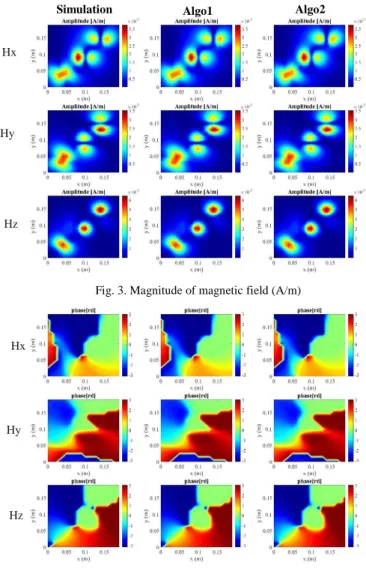
Fig.3 and Fig.4 represent the cartographies of the magnetic field calculated analytically (simulation) and calculated by the model found after optimization using both algorithms (Algo1, Algo2).
Fig. 3. Magnitude of magnetic field (A/m)
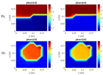
Fig. 4. Phase of magnetic field (rad)
A good agreement is noticeable between the cartographies of magnetic field calculated analytically and those found by the optimization algorithms.
To further evaluate the speed of each optimization algorithm, the computing time is calculated to find an N number of magnetic dipoles by each algorithm. After resolution, both algorithms find a model composed of N magnetic dipoles with a fitness function and 𝛥𝑓 values less than 0.1%.
The following figure represents the computing time of each algorithm as a function of dipoles number (N).
Fig. 5. Calculating time in function of the number of dipoles for both algorithms
As a result, the developed method is clearly faster than the standard optimization algorithm proposed in literature.
III. EXPERIMENTAL VALIDATION OF THE PROPOSED METHOD A. Study of coils radiation
To experimentally validate our method, a mono turn coil, as shown in Fig. 6, printed on a circuit board and a toroidal coil, as shown in Fig. 7, are considered.
Fig. 6. Mono turn coil Fig. 7. Toroidal coil
The following table represents the characteristics of each device and the measurement conditions.
TABLE I
CHARACTERISTICS OF USED DEVICES AND MEASUREMENT CONDITIONS
A near field bench shown in Fig.8 is used to perform the measurements. It includes a 3-axis robot that moves the magnetic probe over a DUT. This probe is generally composed of a loop, which generates a voltage from the varying magnetic flux. A PC makes the acquisition of data measured through a vector network analyzer (VNA). To improve the sensitivity of the measurements, a low noise amplifier is connected at the output of the probe.
Mono turn coil Toroidal coil
Inner radius 24.5 mm 17.8 mm Outer radius 25.5 mm 30.5 mm Thickness 34 um 20 mm Number of turns 1 18 Scanning resolution 20 mm 20 mm Scanning area 200 mm 200 mm 200 mm 200 mm Measurement distance above the DUT
42 mm 40 mm Frequency 10 MHz 10 MHz Hx Hy Hz Hx Hy Hz
Fig. 8. Near-field bench
From the measurements of the magnetic field radiated by the mono turn coil shown in Fig.5, our method determines a model composed of 7 magnetic dipoles where the fitness function equals to 7.4% and 𝛥𝑓 less than 0.1%.
Fig.9 and Fig.10 represent the magnitude and phase of the measured magnetic field and the one found by the model.
Fig. 9. Magnitude of magnetic field (A/m)
Fig. 10. Phase of magnetic field (rad)
Looking at the cartographies of the measured magnetic field and the one given by the model, there is a good agreement in regions with a strong field, in magnitude and phase. To quantify the results, we used the feature selective validation (FSV) [20]. The FSV theory was conceived as a technique to quantify the comparison of data sets by mirroring the perceptions of engineers. The application of FSV to the validation of data is a key element in a current IEEE Standard under development as a means of describing quality of electromagnetic simulation results [20]. In this paper, this tool was used to compare the result of magnetic field components (magnitude, phase) measured and given by the proposed model. The FSV method is based on the separation of the data to be compared into two groups: the first one discusses the difference in amplitude (Amplitude Difference Measure, ADM) and the second one the difference between the characteristics of the signal (Feature Difference Measure, FDM). The combination of these two indicators (ADM and FDM) is a measurement of the overall difference (Global Difference Measure, GDM). The range of values for the ADM, the FDM and GDM can be divided into six categories, each with a natural language descriptor as it is presented in TABLE II. The confidence histogram, like a probability density function, provides some information such as how much emphasis can be placed on the single figure of merit [20].
TABLE II FSV INTERPRETATION SCALE FSV value (quantitative) FSV interpretation (qualitative) FSV value ≤ 0.1 Excellent 0.1 ≤ FSV value < 0.2 Very good 0.2 ≤ FSV value < 0.4 Good 0.4 ≤ FSV value < 0.8 Fair 0.8 ≤ FSV value < 1.6 Poor
1.6 ≤ FSV value Very poor
Measurement Model Model Measurement Hx Hy Hz Hx Hz Hy
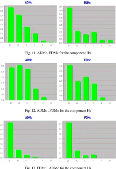
Fig.11, Fig.12 and Fig.13 represent the changes of the FSV results for the three components of the magnetic field radiated by the mono turn coil.
Fig. 11. ADMc, FDMc for the component Hx
Fig. 12. ADMc , FDMc for the component Hy
Fig. 13. FDMc , ADMc for the component Hz
The ADM, FDM and global difference measure (GDM: combination of ADM and FDM) are presented in TABLE.II for the three magnetic field components.
TABLE III
ADM, FDM, GDM RATE FOR THE MAGNETIC FIELD COMPONENTS
The results of the comparison between measurements and computations are good in general for the three components of the magnetic field.
To test the robustness of the proposed method and its effectiveness in finding the equivalent radiating model, a toroidal coil has been studied. This toroidal coil consists of a coil wound around a toroidal ferrite, as shown in Fig.7.
Using the measurements of magnetic field radiated by the toroidal coil, our method finds a model composed of 10 magnetic dipoles where the fitness function equals to 7% and
𝛥𝑓 less than 0.1%.
Fig.14 and Fig.15 represent the components of the magnitude and the phase of the measured magnetic field and the one found by the model.
Fig. 14. Magnitude of magnetic field (A/m)
Fig. 15. Phase of magnetic field (rad)
We notice a very good agreement everywhere between
ADM FDM GDM
Hx 0.205
“ Good” “ Good” 0.275 “ Good” 0.37
Hy 0.221 “ Good” 0.239 “ Good” 0.353 “ Good” Hz 0.079
“ Excellent” “Very Good” 0.104 “Very Good” 0.140
Measurement Measurement Model Model Hz Hx Hy Hz Hx Hy
cartographies. To quantify the results found by the model, the FSV tool is used.
Fig.16, Fig.17 and Fig.18 represent the changes of the FSV measurements for the three components of the magnetic field radiated by the toroidal coil.
Fig. 16. FDMc , ADMc for the component Hx
Fig. 17. FDMc , ADMc for the component Hy
Fig. 18. FDMc , ADMc for the component Hz
The ADM, FDM and GDM are presented in TABLE IV for the three magnetic field components.
TABLE IV
ADM, FDM, GDM RATE FOR THE MAGNETIC FIELD COMPONENTS
Validation tests on the model have shown that measurement data and the simulation results are in good agreement for two components (Hx, Hy) and in excellent agreement for the component Hz.
B. Study of a DC/DC converter radiation
To experimentally validate our method on a real world case, we choose to study the emission of a DC/DC converter (switching mode power supply “SMPS”). It is used to regulate the voltage of electronic circuits especially for unstable input voltage. Fig.19 represents the DC/DC converter used and its electrical circuit.
Fig. 19. DC/DC converter
The following table represents the characteristics of the DC/DC converter.
TABLE V
CHARACTERISTICS OF THE DC/DC CONVERTER
Due to the sensitivity of the VNA, the measurement cannot be done at a frequency below 1 MHz. That is why our measurements have been made at the frequency of 5.7 MHz (19th harmonic) which has the most important amplitude.
The following table represents the measurement conditions.
TABLE VI
MEASUREMENT CONDITIONS
From the measurements of the magnetic field radiated by DC/DC converter shown in Fig.19, our method found a model composed of 15 magnetic dipoles where the fitness function equals to 6 % and 𝛥𝑓 less than 0.1%.
Fig.20 and Fig.21 represent the magnitude and phase of the measured magnetic field and the one found by the model.
ADM FDM GDM
Hx 0.186
“Very Good” “Very Good” 0.156 “Good” 0.258
Hy 0.176
“Very Good” “Very Good” 0.157 “Good” 0.252
Hz 0.054 “Excellent” “Excellent” 0.061 0.088 “Excellent” DC/DC converter Power 3 W Input voltage 48 V Output voltage 5 V Input current 0.7 A Output current 0.6 A Load 9.4 Ω Switching frequency 300 kHz DC/DC converter Scanning resolution 8.5 mm Scanning area 127.5 mm 127.5 mm Measurement distance above the DUT 40 mm
Fig. 20. Magnitude of magnetic field (A/m)
Fig. 21. Phase of magnetic field (rad)
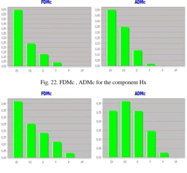
A very good agreement between cartographies can be observed in magnitude and phase. It is confirmed that the equivalent dipoles provides a good representation of the radiation of the DC/DC converter. To quantify the results found by the model, the FSV tool is used. Fig.22, Fig.23 and Fig.24 represent the changes of the FSV measurements for the three components of the magnetic field.
Fig. 22. FDMc , ADMc for the component Hx
Fig. 23. FDMc , ADMc for the component Hy
Fig. 24. FDMc , ADMc for the component Hz
The ADM, FDM and GDM are presented in TABLE.VII for the three magnetic field components.
TABLE VII
ADM, FDM, GDM RATE FOR THE MAGNETIC FIELD COMPONENTS
Validation tests on the model confirm that the equivalent dipoles are a good representation of the DC/DC converter.
It is possible to generalize the model throughout the frequency band under the assumption that the magnetic dipoles position does not change. The magnetic dipoles moments can be calculated as follows:
In this example, we find a model equivalent to the DC/DC converter composed of 15 magnetic dipoles at the frequency 5.7 MHz. Then, the magnetic field radiated by the model at this frequency is written in (1).
ADM FDM GDM
Hx 0.125
“Very Good” “Very Good” 0.118 “Very Good” 0.182 Hy 0.241 “ Good” 0.211 “Good” 0.344 “Good” Hz 0.061 “Excellent” 0.066 “Excellent” 0.095 “Excellent” Measurement Measurement Model Model Hz Hx Hz Hx Hy Hy
The equivalent model of the DC/DC converter at a different frequency (f) can be deduced without passing through an optimization algorithm as following:
𝑯𝒇= 𝑃𝑓𝑴𝒇 (5)
where, 𝑯𝒇 is the magnetic field measured at the frequency f. Under our assumption about the magnetic dipoles positions. We can easily calculate 𝑃𝑓 (matrix depends of magnetic dipoles positions and frequency).
After that, we can directly deduce the moment of magnetic dipoles composed the equivalent model to DC/DC converter at the frequency f by this relation:
𝑴𝒇= 𝑃𝑓−1𝑯𝒇 (6)
In case that our assumption is not valid, the model of the DUT changes in function of the frequency, we are forced to pass again through an optimization algorithm to find the equivalent model.
IV. CONCLUSION
An efficient method has been presented for modeling radiated emissions of a DUT based on near field measurements using an array of equivalent dipoles deduced from an optimization procedure. This method has been inspired from two methods previously proposed. By combining these two methods, the equivalent model is obtained with a reduced number of dipoles in a reduced computing time. Numerical results have shown that the proposed method can reproduce in a satisfying way the radiated fields in a reduced computing time with regards to standard optimization methods.
Finally, the method has been firstly experimentally tested in cases of a mono turn coil and a toroidal coil in near field. The results given by the obtained models show a good agreement with the magnetic field measurements. In addition, the method has been tested on a real complex case (DC/DC converter). The algorithm has shown its effectiveness and has given a model with a good agreement compared to the magnetic field measurements.
In future works, the model will be generalized and used in different shielding applications.
REFERENCES
[1] L. Beghou, B. Liu, L. Pichon and F. Costa, " Synthesis of equivalent
3-D models from near field measurements – Application to the EMC of power printed circuit boards", IEEE Trans. on Magnetics, vol. 45, pp. 1650-1653, March 2009.
[2] A. Frikha, M. Bensetti, F. Duval, N. Benjelloun, F. Lafon, and L.Pichon,
“A New Methodology to Predict the Magnetic Shielding effectiveness of Enclosures at Low Frequency in the Near Field,” IEEE Trans. Magnetics, vol.51, no. 3, pp. 1-4, Mar. 2015.
[3] A. Frikha, M. Bensetti, F. Duval, F. Lafon, L. Pichon, ''Prediction of the
Shielding Effectiveness at Low Frequency in Near Magnetic Field'', Eur. Phys. J. Appl. Phys. 66: 10904, 2014.
[4] A. Frikha, M. Bensetti, F. Duval, F. Lafon, and L.Pichon, '' Modeling of
the Shielding Effectiveness of Enclosures in Near Field at Low Frequencies '', International Conference on Electromagnetics in Advanced Applications (ICEAA'13), Torino, Italy, September 2013.
[5] X. Tong, D. W. P. Thomas, A. Nothofer, P. Sewell, and C. Christopou-
los, “Modeling electromagnetic emissions from printed circuit boards
in closed environments using equivalent dipoles,” IEEE Trans. Electromagn. Compat., vol. 52, no. 2, pp. 462–470, May 2010.
[6] Y. Vives-Gilabert, C. Arcambal, A. Louis, F. de Daran, P. Eudeline, and
B. Mazari, “Modeling magnetic radiations of electronic circuits using near-field scanning method,” IEEE Trans. Electromagn. Compat., vol. 49, no. 2, pp. 391–400, May 2007.
[7] Z. Yu, J. Koo, J. A. Mix, K. Slattery, and J. Fan, “Extracting physical IC
models using near-field scanning,” in Proc. IEEE Int. Symp. Electromagn. Compat., Fort Lauderdale, FL, Jul. 25–30, 2010, pp. 317–320.
[8] J. Regue´, M. Ribo´, J. Garrell, and A. Mart´ın, “A genetic algorithm based
method for source identification and far-field radiated emissions prediction from near-field measurements for PCB characterization,” IEEE Trans. Electromagn. Compat., vol. 43, no. 4, pp. 520–530, Nov. 2001.
[9] J. J. Laurin, J. F. Zürcher, and F. E. Gardiol, “Near-Field Diagnostics of Small Printed Antennas Using the Equivalent Magnetic Current Approach,” IEEE Trans. Antennas Propagat., vol. 49, no. 5, pp 814-828, May, 2001.
[10] B. Ravelo, Y. Liu, A. Louis, and A. K. Jastrzebski, “Study of high-frequency electromagnetic transients radiated by electric dipoles in near- field,” IET Microw. Antennas Propag., vol. 5, pp. 692–698, 2011.
[11] Z. Song, S. Donglin, F. Duval, A. Louis, and D. Fei, “A novel electromag- netic radiated emission source identification methodology,” in Proc. Asia- Pacific Symp. Electromagn. Compat., Pekin, China, Apr. 12–16, 2010, pp. 645–648.
[12] B. Essakhi, D. Baudry, O. Maurice, A. Louis, L. Pichon, and B. Mazari, “Characterization of radiated emissions from powerelectronic devices: Synthesis of an equivalent model from near-field measurement,” Eur. Phys. J. Appl. Phys., vol. 38, pp. 275–281, 2007.
[13] S. Saidi and J. Ben Hadj Slama, “A Near-Field technique based on PZMI, GA, and ANN: Application to power electronics systems,” IEEE Trans. Electromagn. Compat., vol. 56, no. 4, pp. 784–791, Aug. 2014.
[14] T. S. Sijher and A. A. Kishk, “Antenna modeling by infinitesimal dipoles using genetic algorithms,” Progress Electromagn. Res., vol. 52, pp. 225– 254, 2005.
[15] B. Liu, L. Beghou, and L. Pichon, “Adaptive genetic algorithm based source identification with Near-Field scanning method,” Progress Elec- tromagn. Res. B, vol. 9, pp. 215–230, 2008.
[16] J. R. Regue´, M. Ribo´, J. M. Garrell, and A. Mart´ın, “A genetic algorithm based method for source identification and Far-Field radiated emissions prediction from near-field measurements for PCB characterization,” IEEE Trans. Electromagn. Compat., vol. 43, no. 4, pp. 520–530, Nov. 2001. [17] X. Tong, D W P Thomas, K. Biwojno, A. Nothofer, P. Sewell, and C.
Christopoulos, "Modeling Electromagnetic Emissions from PCBs in Free Space Using Equivalent Dipoles", Proceedings of the 39th European Microwave Conference, pp. 280-283, October 2009.
[18] D. Baudry, F. Bicrel, L. Bouchelouk, A. Louis, B. Mazari, and P. Eudeline,“Near-field techniques for detecting EMI sources”, in Proc. IEEE Int. Symp. EMC, Santa Clara, CA, vol. 1, pp. 11–13, August 2004. [19] H. Shall, Z. Riah, and M. Kadi, ''A 3D near-field modeling approach for
electromagnetic prediction, '' IEEE Trans. Electromagn. Compat,.vol. 56, pp. 102-112, February 2014.
[20] A. P. Duffy, A. J. Martin, A. Orlandi, G. Antonini, T. M. Benson, and M. S. Woolfson, “Feature selective validation (FSV) for validation of computational electromagnetics (CEM). Part I—the FSV method,”IEEE Trans. Electromagn. Compat., vol. 48, no. 3, pp. 449–459, Aug. 2006. [21] W. Abdelli, X. Mininger, L. Pichon, H. Trabelsi, "Prediction of Radiation
from Shielding Enclosures using Equivalent 3D High Frequency Models", IEEE Trans. on Magnetics, Volume 51, Issue 3, May 2015. [22] W. J. Zhao, B. F. Wang, E. X. Liu, H. B. Park, H. H. Park, E. Song, and
E. P. Li, “An Effective and Efficient Approach for Radiated Emission Prediction Based on Amplitude-Only Near-Field Measurements,” IEEE Trans. Electromagn. Compat., vol. 54, no. 5, pp. 1186–1189, Oct. 2012. [23] A. Frikha, M. Bensetti, L. Pichon, F. Lafon , F. Duval, and N.Benjelloun
'' Magnetic Shielding Effectiveness of Enclosures in Near Field at Low
Frequency for Automotive Applications,'' IEEE Trans.
[24] Li, Liang, "Radiation noise source modeling and near-field coupling estimation in RF interference," (2016). Masters Theses. 7558. http://scholarsmine.mst.edu/masters_theses/7558