HAL Id: hal-01395449
http://hal.univ-nantes.fr/hal-01395449
Submitted on 7 Dec 2019
HAL is a multi-disciplinary open access
archive for the deposit and dissemination of
sci-entific research documents, whether they are
pub-lished or not. The documents may come from
teaching and research institutions in France or
abroad, or from public or private research centers.
L’archive ouverte pluridisciplinaire HAL, est
destinée au dépôt et à la diffusion de documents
scientifiques de niveau recherche, publiés ou non,
émanant des établissements d’enseignement et de
recherche français ou étrangers, des laboratoires
publics ou privés.
How to benchmark objective quality metrics from paired
comparison data?
Philippe Hanhart, Lukáš Krasula, Patrick Le Callet, Touradj Ebrahimi
To cite this version:
Philippe Hanhart, Lukáš Krasula, Patrick Le Callet, Touradj Ebrahimi. How to benchmark objective
quality metrics from paired comparison data?. 8th International Conference on Quality of Multimedia
Experience (QoMEX), Jun 2016, Lisbon, Portugal. �10.1109/QoMEX.2016.7498960�. �hal-01395449�
How to Benchmark Objective Quality Metrics from
Paired Comparison Data?
Philippe Hanhart
∗, Luk´aˇs Krasula
†‡, Patrick Le Callet
†, and Touradj Ebrahimi
∗†Multimedia Signal Processing Group, EPFL, Lausanne, Switzerland †LUNAM University - IRCCyN CNRS UMR 6597, 44306, Nantes, France ‡Czech Technical University in Prague, Technick´a 2, 166 27 Prague 6, Czech Republic
Abstract—The procedures commonly used to evaluate the performance of objective quality metrics rely on ground truth mean opinion scores and associated confidence intervals, which are usually obtained via direct scaling methods. However, indirect scaling methods, such as the paired comparison method, can also be used to collect ground truth preference scores. Indirect scaling methods have a higher discriminatory power and are gaining popularity, for example in crowdsourcing evaluations. In this paper, we present how the classification errors, an existing analysis tool, can also be used with subjective preference scores. Additionally, we propose a new analysis tool based on the receiver operating characteristic analysis. This tool can be used to further assess the performance of objective metrics based on ground truth preference scores. We provide a MATLAB script with an implementation of the proposed tools and we show one example of application of the proposed tools.
I. INTRODUCTION
The most important step in the development process of an objective quality metric is its verification with regards to subjective data. Indeed, it is essential to verify that the model can reliably and accurately predict perceived visual quality. This verification process is essential to assess the performance of an objective quality metric, to determine its scope of validity, and to compare its performance against other metrics. For this purpose, ground truth subjective quality scores obtained via subjective visual quality experiments are used.
In the classical performance evaluation framework for ob-jective metrics [1], a regression is first fitted to map the metric scores to the mean opinion scores (MOSs). Then, different performance indexes are computed to evaluate the metric’s performance. In particular, the Pearson and Spearman correla-tion coefficients, root-mean-square error, and outlier ratio are computed to estimate the linearity, monotonicity, accuracy, and consistency of the metric’s estimation of MOS, respectively. Finally, to compare the performance of two metrics, their performance index values are compared using statistical tests. Because of the classical performance evaluation procedure, almost all public image and video databases for quality assess-ment [2] were obtained using a test method that consists of a direct scaling of the stimuli, e.g., the ACR/SS, DCR/DSIS, or DSCQS test methods [3], [4] to obtain MOS (of differ-ential MOS). Reciprocally, most performance evaluations of objective quality metrics, such as the studies from Sheikh
The work presented in this paper was possible thanks to COST Action IC1003 (Qualinet).
et al. [5] for image quality assessment and the study from Seshadrinathan et al. [6] for video quality assessment, rely on ground truth MOS.
Despite the popularity of direct scaling methods, indirect scaling methods, e.g., the paired comparison (PC), have a higher discriminatory power, which is of particular value when visual differences between stimuli are small. Additionally, indirect scaling methods are also sometimes preferred since it is easier for subjects to select which image or video has better quality in a pair rather than to relate the quality of an image or a video to a particular quality level on a given scale. This is the reason why indirect scaling methods are preferred for some applications, e.g., the evaluation of rendering algorithms or scalable video coding algorithms. In summary, indirect scaling is more natural and requires little to no training while providing more reliable results, which is particularly beneficial for crowdsourcing evaluations for example.
There are very few databases for quality assessment that were obtained using the PC method. The major exceptions are the TID2008 [7] and TID2013 [8] databases, which were created using a test methodology derived from the PC method. However, the subjective scores provided in the TID databases still consist of MOS, which were derived from the different comparisons. Another exception is the EPFL scalable video database [9], which was created using both the PC method by considering all possible pairs and the more standard SSCQS method. Despite that both PC and MOS values are provided in the EPFL database, most papers that use this database to benchmark objective metrics only use the MOS values. The only exception is the work from Demirtas et al. [10], where the PC scores were converted to MOS-like scores using the Bradley-Terry-Luce (BTL) model [11], [12]. To evaluate the metrics performance, the authors considered three test images, each created from the same reference image using the same distortion, and checked whether the ranking of these images was the same based on the metric scores as on the BTL scores. Another approach was used in [13] and [14], where the PC method was used to evaluate the quality of high dynamic range image and video content, respectively. The PC scores were first converted to MOS-like scores using the Thurstone Case V model [15], which is a precursor of the BTL model. Then, the Thurstone scores were converted to the range [1, 5] by mapping the lowest and highest quality score values to 1 and 5, respectively, based on the fact that the lower and upper bit rates were selected to be representative of the lowest and best quality. Finally, a classical performance evaluation was performed considering the Thurstone scores as MOSs.
The major problem is that the Thurstone and BTL models provide relative scores only for stimuli that have been directly compared. Even if there are ways to infer scores from indirect comparisons, i.e., to estimate MOS-like scores from incom-plete PC designs, it is not meaningful to compare different image or video contents to avoid the problem of mapping BTL scores of different contents to a common scale. Apart from the comparisons between contents, some comparisons within con-tent but between different cases, e.g., algorithms or resolution, are also not meaningful. Therefore, instead of converting pref-erence scores to MOS-like scores using the Thurstone or BTL models, in this paper, we propose to use alternative procedures that can be applied directly on the subjective preference scores. In particular, we propose to first classify the pairs into two categories based on the outcome of the subjective evaluation: pairs with significant differences and pairs without significant differences. To test the significance of preference scores, several tests can be applied, such as the Barnard’s test [16] or the binomial test. Then, the frequencies of classification errors can be computed according to recommendation ITU-T J.149 [17] by varying a threshold on the objective scores while comparing the outcome of the metric’s classification to that of the subjective evaluation. Even though the procedure was originally proposed for subjective scores collected via direct scaling methods, it can also be applied for indirect scaling methods since it only considers the output of a comparison between two stimuli. We suggest a statistical test that can be used to compare the classification errors of two metrics. Additionally, we present a new analysis tool inspired from the classification errors and receiver operating characteristic (ROC) analyses. The proposed analysis tool considers only two classes, instead of three in the classification errors analysis, as the ROC analysis was designed for binary classification systems. Similarly to the classification errors analysis, a thresh-old on the objective scores is varied while recording the true positive and false positive rates. To have a better understanding at the metric’s performance in the different situations, we suggest performing three separate ROC analyses to consider all meaningful cases. To compare the ROC curves of two metrics, we suggest comparing the area under the curve (AUC) of the corresponding ROC curves. We use a common statistical test to compare the AUC values of two metrics. We believe that the classification errors and proposed ROC analyses pro-vide a meaningful way to benchmark objective metrics from preference scores, without the need to convert them to MOS-like values. A MATLAB script to easily apply the proposed analysis tools can be downloaded via the following DOI link: https://doi.org/10.5281/zenodo.50493
The remainder of this paper is organized as follows. Differ-ent possible analysis tools to evaluate objective metrics from PC data are described in Sec. II. An example of application of the analysis tools is presented in Sec. III. Finally, concluding remarks are given in Sec. IV.
II. ANALYSISTOOLS
First, a statistical test is applied to the subjective preference scores collected from the different observers to classify the stimuli into pairs with and without significant differences. Then, the classification errors and proposed ROC analyses are performed. Finally, statistical tests are applied to test for the significance of the difference between two metrics.
Table I: Classification errors.
Objective Subjective
A > B A = B A < B A > B Correct Decision False Differentiation False Ranking A = B False Tie Correct Decision False Tie A < B False Ranking False Differentiation Correct Decision
A. Analysis of Subjective Preference Scores
The individual preference scores collected using the PC [4] or stimulus comparison [3] method first need to be processed to determine whether the preference for one stimulus over the other is statistically significant. First, the subjective preference scores need to be arranged in only two classes, which is straightforward if a binary scale is used. If a ternary scale is used, then the ties can be split equally between the two preference options. For other scales, such as the comparison scale (Much worse, Worse, Slightly worse, The same, Slightly better, Better, and Much better), weights can be associated with the different labels. For example, a count of 0.5, 1, and 1.5 could be added to the corresponding preference option for Slightly better/Slightly worse, Better/Worse, and Much better/Much worse, respectively, whereas a count of 0.5 could be added to both preference options for The same.
This data roughly follows a Bernoulli process B(N, p), where N is the sum of all individual counts and p is the probability of success in a Bernoulli trial, which is set to 0.5, considering that, a priori, both options have the same chance of success. The binomial cumulative distribution function is then used to determine the critical region for the statistical test.
Other statistical tests, e.g., the Barnard’s test [16], can also be used to determine whether preference for one stimulus over the other is statistically significant. The Barnard’s test is a statistical significance test of the null hypothesis of independence of rows and columns in a 2 × 2 contingency table. Thus, this statistical test can also be used to test whether the preference probability is statistically significantly different from 0.5.
B. Classification Errors
In recommendation ITU-T J.149 [17], it is suggested to compute the classification errors to evaluate the performance of an objective metric. A classification error is performed when the objective metric and subjective evaluation lead to different conclusions on a pair of stimuli, A and B, for example. Three types of error can happen (see Table I)
1) False Tie, the least offensive error, which occurs when the subjective evaluation says that A and B are different, whereas the objective scores say that they are identical, 2) False Differentiation, which occurs when the subjective
evaluation says that A and B are identical, whereas the objective scores say that they are different,
3) False Ranking, the most offensive error, which occurs when the subjective evaluation says that A (B) is better than B (A), whereas the objective scores say the opposite. The percentage of Correct Decision, False Tie, False Dif-ferentiation, and False Ranking are recorded from all possible distinct pairs as a function of the difference in the metric values, ∆OM .
As ∆OM increases, more pairs of data points are consid-ered as equivalent by the objective metric. This reduces the occurrences of False Differentiations and False Rankings, but increases the occurrence of False Ties. On the other hand, as ∆OM tends towards 0, the occurrence of False Tie will tend towards 0, while the occurrence of False Differentiation will tend towards the proportion of pairs of data points where there was not enough evidence to show a statistical difference in the subjective evaluation.
The relative frequencies are plotted as a function of the significance threshold ∆OM . Ideally, the occurrence of Cor-rect Decision should be maximized and the occurrence of False Ranking should be minimized when the ∆OM tends towards 0. The occurrences of False Differentiations and False Rankings should decrease as fast as possible as ∆OM increases. Based on this, different graphs corresponding to different metrics can be compared to determine the best metric for the application under analysis.
Since comparing numbers is easier than comparing graphs, let us consider two important cases. The first case is when ∆OM = 0, i.e., when any increase (decrease) in the metric’s score is assumed to lead to a visible increase (decrease) in visual quality. Even though it is not reasonable to assume that any change in objective score leads to a visible difference in visual quality, this is unfortunately how many people use objective metrics. Indeed, it is quite common to see scientific papers claiming better performance for a particular algorithm for gains as low as 0.1dB in PSNR. Thus, by studying the classification errors of the objective metric for ∆OM = 0, we know how many False Differentiation errors are made in this case. The other important case is for the ∆OM value that maximizes the Correct Decision frequency. This point indicates the highest percentage of agreement between the objective metric and the subjective test and can be used to determine a threshold on the metric score difference.
C. Significance of the Difference between Correct Decisions We suggest to use a statistical test to compare the best Correct Decision rates of two different metrics. Note that the same statistical test can also be applied to compare Correct Decision rates corresponding to other ∆OM values than the ones that maximize the Correct Decision rates, e.g., for ∆OM = 0, or to compare Correct Decision rates of the same metric but for two different values of ∆OM . Also, the same statistical test can be applied for the False Tie, False Differentiation, and False Ranking.
There is a number of statistical tests applicable for bino-mial variables comparison described in the literature. They are based on different assumptions and can provide differ-ent powers under certain circumstances. Suitable methods include Chernoff bound [18] and Pinsker’s inequality [19]. Fisher’s [20] and Barnard’s [16] exact tests can be used as well. The comparison of these techniques would require a separate study and exceeds the scope of this paper.
Here, we use the same test as the one suggested in [1] for testing the significance of the difference between two OR values. The Correct Decision (CD) follows a binomial distribution with mean p = CD and standard deviation σp=
q
p(1−p)
N , where N is the total number of pairs.
To determine whether the difference between two Correct Decision values corresponding to two different objective met-rics is statistically significant, a two-sample statistical test is performed. The null hypothesis under test is that there is no significant difference between Correct Decision values, against the alternative hypothesis that the difference is significant, although not specifying better or worse.
If the sample size is large (N ≥ 30), then the distribution of differences of proportions from two binomially distributed populations can be approximated by a normal distribution according to the central limit theorem. The observed value zobs computed from the observations for each comparison is
zobs = σp1−p2 p1−p2 with σp1−p2 = q p(1 − p)2 N and p = p1+p2 2
because the null hypothesis in this case considers that there is no difference between the population parameters p1and p2. If
the observed value zobsis inside the critical region determined
by the 95% two-tailed z-value, then the null hypothesis is rejected at a 5% significance level.
D. Receiver Operating Characteristic
The ROC curve illustrates the performance of a binary classifier system as its discrimination threshold is varied. However, when comparing a pair of stimuli, A and B, there are three possible outcomes: A < B, A = B, or A > B. Hence, the outcome of the comparison is ternary and a direct ROC analysis cannot be performed. Therefore, we suggest performing three separate ROC analyses where only binary classification is considered
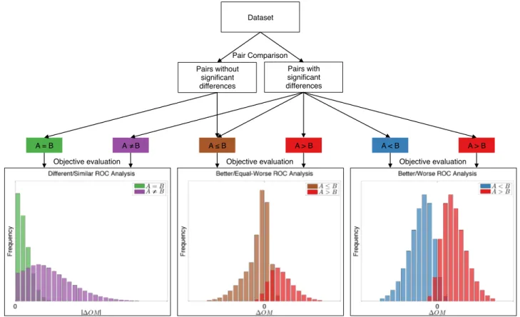
1) Different/Similar ROC Analysis: this analysis illustrates the ability of the metric to discriminate between signifi-cant and not signifisignifi-cant visual quality differences in a pair of stimuli. In this case, all data points are considered. 2) Better/Worse ROC Analysis: this analysis illustrates the
ability of the metric to determine which stimulus in a pair has the best visual quality. In this case, only data points corresponding to pairs with significant difference are considered.
3) Better/Equal-Worse ROC Analysis: this analysis illus-trates the ability of the metric to determine whether stim-ulus A has similar or worse visual quality than stimstim-ulus B or if it has significantly better visual quality than stimulus B. In this case, all data points are considered.
Figure 1 illustrates the procedure. First, the dataset is split into pairs with and without significant differences in terms of visual quality based on the pair comparison test. Then, different classes, namely, A = B, A 6= B, A < B, A > B, and A ≤ B are formed. For each ROC analysis, the histogram of the two corresponding classes is constructed as a function of the metric difference ∆OM between the two stimuli. Note that for the Different/Similar ROC Analysis, the absolute metric difference is used. For the two other ROC analyses, the data is repeated to have both AB and BA pairs. The discrimination threshold is set on ∆OM and varied while recording the true positive rate (TPR) and false positive rate (FPR). Finally, the ROC curve is built by plotting TPR as a function of FPR.
Note that this analysis tool can also be used with ground truth MOS scores, as illustrated in [21].
Pairs without significant differences! Pairs with significant differences! A = B! A ≠ B! A ≤ B! A > B! A < B! A > B! Dataset! Pair Comparison!
Objective evaluation! Objective evaluation! Objective evaluation!
Figure 1: ROC analysis: creation of the different classes.
Table II: ROC analysis properties.
ROC Analysis H0 H1 TPR=FPR=1 TPR=FPR=0
Different/Similar A = B A 6= B |∆OM | = 0 |∆OM | → +∞ Better/Worse A < B A > B ∆OM → −∞ ∆OM → +∞ Better/Equal-Worse A ≤ B A > B ∆OM → −∞ ∆OM → +∞
The ROC curves can be compared visually to determine which metric performs better, considering that the point in the top left corner of the ROC space corresponds to a perfect classification. A completely random guess would give a point along the diagonal line from the bottom left to the top right corners. The top right and bottom left corners correspond to the smallest and largest ∆OM values, respectively, as specified in Table II. Note that the TPRs for ∆OM = 0 are the same for the Better/Worse and Better/Equal-Worse ROC analyses, as they have the same class for the alternative hypothesis. However, for ∆OM = 0, the FPR of the Better/Equal-Worse ROC analysis is greater than or equal to the FPR of the Better/Worse ROC analysis, as the class for the null hypothesis of the Better/Equal-Worse ROC analysis also contains the data corresponding to pairs without significant differences. Note also that the Better/Worse ROC curve is symmetric about the diagonal line from the bottom right to the top left corners, as the two classes are symmetric about ∆OM = 0 since both AB and BA pairs are considered. The Better/Equal-Worse ROC analysis relies on both abilities to discriminate between significant and not significant visual quality differences in a pair of stimuli and to determine which stimulus in a pair has the best visual quality for pairs with significant visual quality differences. Therefore, the Better/Equal-Worse ROC curve typically lies between the Different/Similar and Better/Worse
ROC curves. If the three curves are well separated, then the metric is better at discriminating between significant and not significant visual quality differences than at determining which stimulus has the best visual quality (or the other way around, depending on which ROC curve lies above the other ones).
Even though the ROC curve provides a lot of informa-tion, it is easier to compare a simple number that represents some characteristics of the ROC curve. A commonly used performance indicator is the area under the curve (AUC). The AUC value is between 0 and 1; the higher the better. Therefore, it is possible to compare metrics by comparing their AUC values. Another important indicator is the percentage of correct classification, i.e., the accuracy, for ∆OM = 0 for the Better/Worse ROC analysis. Indeed, a metric can have higher AUC, but lower correct classification, as discussed in [21]. E. Significance of the Difference between Areas Under the Curve
Various tests to determine the significance of the difference between two AUC values have been proposed. The methods can be parametric [22] or non-parametric [23]. More recently, techniques based on bootstrap have been proposed as well [24]. Similarly to Sec. II-C, comparison of the different approaches exceeds the scope of this paper. Most statistical toolboxes and packages implement several methods for both paired and un-paired ROC curves. In our example, we use the popular method proposed by DeLong et al. [23]. The provided MATLAB script includes the fast implementation of the DeLong’s algorithm proposed in [25], as well as the parametric test proposed by Hanley and McNeil [22].
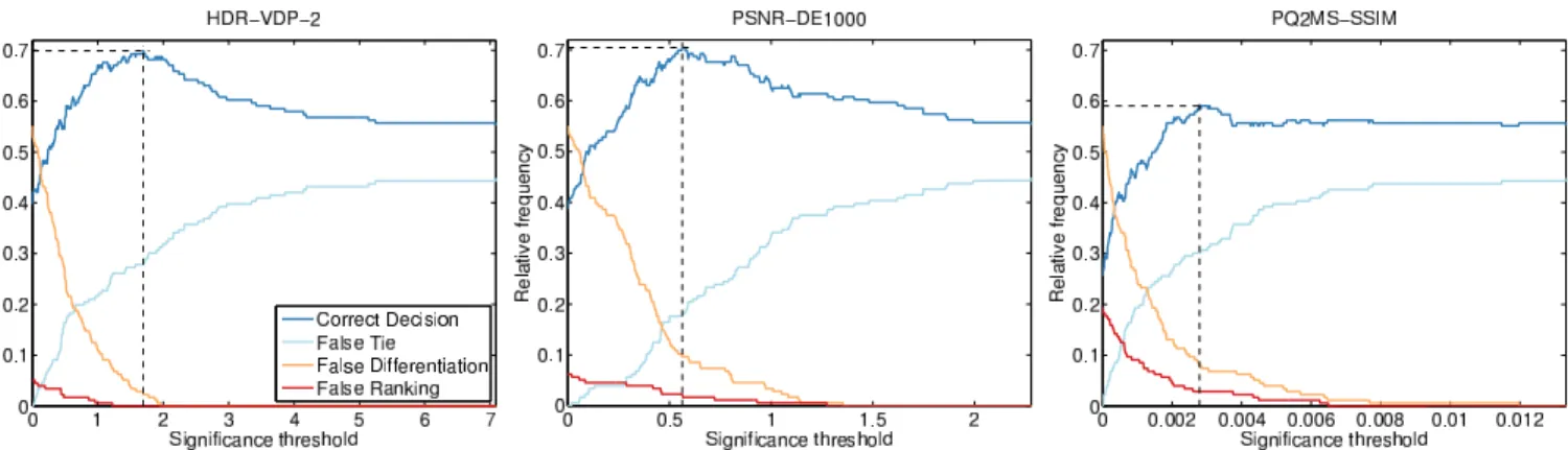
Figure 2: Frequencies of classification error. The dashed lines indicate the ∆OM value that maximizes the Correct Decision.
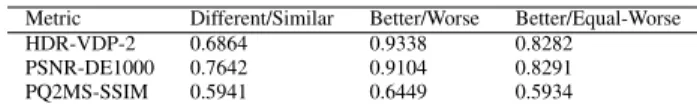
Figure 3: ROC analysis. The dashed lines indicate the TPR and FPR values for ∆OM = 0. III. EXAMPLE
In this section, we show one example of application of the proposed analysis tools. For this purpose, we used a dataset of 5 high dynamic range (HDR) video sequences, which were encoded at 4 bit rates with HEVC HDR Profile and 9 algorithms in competitions submitted in response to the MPEG Call for Evidence on HDR video coding [26]. The subjective evaluations were conducted on a full HD 42” Dolby Research HDR RGB backlight dual modulation display (aka Pulsar). Two video sequences were presented simultaneously in side-by-side fashion. One of the two video sequences was always the HEVC anchor. The other video sequence was the proponent to be evaluated, at the same (targeted) bit rate as the anchor. Subjects were asked to judge which video sequence in a pair (‘left’ or ‘right’) has the best overall quality. The option ‘same’ was also included to avoid random preference selections. In total, 176 paired comparisons were evaluated by 24 subjects. To discriminate between pairs with and without significant differences, a binomial test was performed at 5% significance level. Different objective metrics were computed in the linear and PQ-TF domains. Please refer to [26] for more details.
Figure 2 depicts the classification errors for HDR-VDP-2, PSNR-DE1000, and PQ2MS-SSIM. Table III reports the classification errors for the ∆OM value that maximizes the Correct Decisionfrequency. As it can be observed,
HDR-VDP-Table III: Classification errors for the ∆OM value that maxi-mizes the Correct Decision frequency.
Metric Correct False False False Decision(%) Tie(%) Differentiation(%) Ranking(%) HDR-VDP-2 69.9 27.8 2.3 0.0 PSNR-DE1000 70.5 17.6 9.7 2.3 PQ2MS-SSIM 59.1 30.1 8.0 2.8
2 and PSNR-DE1000 achieve significantly higher Correct De-cisionfrequency than PQ2MS-SSIM (p < 0.05). At the ∆OM value that maximizes the Correct Decision frequency, the difference between the Correct Decision rates of HDR-VDP-2 and PSNR-DE1000 is not significant. However, HDR-VDP-2 can achieve significantly lower False Ranking (p < 0.05) and False Differentiation (p < 0.005) errors than PSNR-DE1000, but at the expense of significantly higher False Tie errors (p < 0.05), which is however the least offensive error.
Figure 3 depicts the ROC curves for HDR-VDP-2, PSNR-DE1000, and PQ2MS-SSIM. Table IV reports the AUC values for the different ROC analyses. As it can be observed, HDR-VDP-2 and PSNR-DE1000 are better at determining which video in a pair has the best visual quality for pairs with significant visible differences than at discriminating between significant and not significant visual quality differences. On the other hand, PQ2MS-SSIM performs about the same in any case, as the three curves are close to each other, and its
Table IV: AUC values for the different ROC analyses.
Metric Different/Similar Better/Worse Better/Equal-Worse HDR-VDP-2 0.6864 0.9338 0.8282
PSNR-DE1000 0.7642 0.9104 0.8291 PQ2MS-SSIM 0.5941 0.6449 0.5934
performance is closer to random, as the curves are closer to the diagonal. From the statistical tests on the AUC values, there is no significant difference between HDR-VDP-2 and PSNR-DE1000 for any of the three ROC analyses. However, HDR-VDP-2 and PSNR-DE1000 significantly outperform PQ2MS-SSIM based on the statistical tests applied on the AUC values for the Better/Equal-Worse and Better/Worse ROC analyses (p < 0.001), while only PSNR-DE1000 significantly outper-form PQ2MS-SSIM for the Different/Similar ROC analysis (p < 0.005).
From the above analysis, it can be concluded that PSNR-DE1000 is a good alternative to HDR-VDP-2, which is much more computationally expensive. On the other hand, the MS-SSIM metric computed in the PQ-TF domain performs signif-icantly lower. This example shows how the proposed analysis tools can be applied to evaluate the performance of objective metrics and to compare the performance of two metrics.
IV. CONCLUSION
Although the PC method is very popular for its discrimi-natory power, the subjective results of such experiments are rarely used for benchmarking objective metrics since they do not provide MOS-like scores, as required by the standard correlation based performance measures. In this paper, we have presented different analysis tools to evaluate and compare the performance of objective metrics from ground truth preference scores. These tools enable to directly use the results obtained in PC experiments for the benchmarking of objective met-rics. In particular, the new analysis tool is based upon the ROC analysis and provides more insights about the metric performance and behavior. Furthermore, we suggested some statistical tests to measure the significance of the difference between two metrics for the analysis tools presented in this paper. We presented one real life example of application of these statistical tools based on a MATLAB script that we have made publicly available to promote the benchmarking of objective metrics from PC data.
REFERENCES
[1] ITU-T P.1401, “Methods, metrics and procedures for statistical eval-uation, qualification and comparison of objective quality prediction models,” International Telecommunication Union, July 2012. [2] S. Winkler, “Analysis of Public Image and Video Databases for Quality
Assessment,” IEEE Journal of Selected Topics in Signal Processing, vol. 6, no. 6, pp. 616–625, Oct. 2012.
[3] ITU-R BT.500-13, “Methodology for the subjective assessment of the quality of television pictures,” International Telecommunication Union, Jan. 2012.
[4] ITU-T P.910, “Subjective video quality assessment methods for mul-timedia applications,” International Telecommunication Union, Apr. 2008.
[5] H. R. Sheikh, M. F. Sabir, and A. C. Bovik, “A Statistical Evaluation of Recent Full Reference Image Quality Assessment Algorithms,” IEEE Transactions on Image Processing, vol. 15, no. 11, pp. 3440–3451, Nov. 2006.
[6] K. Seshadrinathan, R. Soundararajan, A. C. Bovik, and L. K. Cormack, “Study of Subjective and Objective Quality Assessment of Video,” IEEE Transactions on Image Processing, vol. 19, no. 6, pp. 1427–1441, 2010. [7] N. Ponomarenko, V. Lukin, A. Zelensky, K. Egiazarian, M. Carli, and F. Battisti, “TID2008 - A Database for Evaluation of Full-Reference Visual Quality Assessment Metrics,” Advances of Modern Radioelec-tronics, vol. 10, no. 4, pp. 30–45, 2009.
[8] N. Ponomarenko, L. Jin, O. Ieremeiev, V. Lukin, K. Egiazarian, J. Astola, B. Vozel, K. Chehdi, M. Carli, F. Battisti, and C.-C. J. Kuo, “Image database TID2013: Peculiarities, results and perspectives,” Signal Processing: Image Communication, vol. 30, pp. 57–77, 2015. [9] J.-S. Lee, F. De Simone, and T. Ebrahimi, “Subjective Quality
Evalu-ation via Paired Comparison: ApplicEvalu-ation to Scalable Video Coding,” IEEE Transactions on Multimedia, vol. 13, no. 5, pp. 882–893, Oct. 2011.
[10] A. M. Demirtas, A. R. Reibman, and H. Jafarkhani, “Full-Reference Quality Estimation for Images With Different Spatial Resolutions,” IEEE Transactions on Image Processing, vol. 23, no. 5, pp. 2069–2080, May 2014.
[11] R. A. Bradley and M. E. Terry, “Rank analysis of incomplete block designs: I. the method of paired comparisons,” Biometrika, vol. 39, no. 3-4, pp. 324–345, 1952.
[12] R. D. Luce, “Individual choice behaviours: A theoretical analysis,” 1959.
[13] P. Hanhart, M. Bernardo, P. Korshunov, M. Pereira, A. Pinheiro, and T. Ebrahimi, “HDR image compression: A new challenge for objective quality metrics,” in International Workshop on Quality of Multimedia Experience (QoMEX), Sep. 2014.
[14] M. Rerabek, P. Hanhart, P. Korshunov, and T. Ebrahimi, “Subjective and objective evaluation of HDR video compression,” in International Workshop on Video Processing and Quality Metrics for Consumer Electronics (VPQM), Feb. 2015.
[15] L. L. Thurstone, “A law of comparative judgment,” Psychological review, vol. 34, no. 4, p. 273, 1927.
[16] G. A. Barnard, “A new test for 2× 2 tables,” Nature, vol. 156, p. 177, 1945.
[17] ITU-T J.149, “Method for specifying accuracy and cross-calibration of Video Quality Metrics (VQM),” International Telecommunication Union, Mar. 2004.
[18] H. Chernoff, “A measure of asymptotic efficiency for tests of a hypothesis based on the sum of observations,” Annals of Mathematical Statistics, vol. 23, no. 4, pp. 493–507, 1952.
[19] T. M. Cover and J. A. Thomas, Elements of Information Theory, 2nd ed. Willey-Interscience, 2006.
[20] R. A. Fisher, “On the interpretation of χ2from contingency tables, and
the calculation of p,” Journal of Royal Statistical Society, vol. 85, no. 1, pp. 87–94, 1922.
[21] L. Krasula, K. Fliegel, P. Le Callet, and M. Kl´ıma, “On the accuracy of objective image and video quality models: New methodology for performance evaluation,” in International Conference on Quality of Multimedia Experience (QoMEX), June 2016.
[22] J. A. Hanley and B. J. McNeil, “The Meaning and Use of the Area under a Receiver Operating Characteristic (ROC) Curve,” Radiology, vol. 143, no. 1, pp. 29–36, Apr. 1982.
[23] E. R. DeLong, D. M. DeLong, and D. L. Clarke-Pearson, “Comparing the Areas under Two or More Correlated Receiver Operating Charac-teristic Curves: A Nonparametric Approach,” Biometrics, vol. 44, no. 3, pp. 837–845, 1988.
[24] E. S. Venkatraman, “A Permutation Test to Compare Receiver Operating Characteristic Curves,” Biometrics, vol. 56, no. 4, pp. 1134–1138, 2000. [25] X. Sun and W. Xu, “Fast Implementation of DeLong’s Algorithm for Comparing the Areas Under Correlated Receiver Operating Characteris-tic Curves,” IEEE Signal Processing Letters, vol. 21, no. 11, pp. 1389– 1393, 2014.
[26] P. Hanhart, M. Rerabek, and T. Ebrahimi, “Towards high dynamic range extensions of HEVC: subjective evaluation of potential coding technologies,” in Proceedings of SPIE 9599, ser. Applications of Digital Image Processing XXXVIII, Aug. 2015.