Université de Montréal
Factor models, VARMA processes and parameter instability with applications in macroeconomics
par
Dalibor Stevanovi´c
Département des sciences économiques Faculté des arts et des sciences
Thèse présentée à la Faculté des arts et des sciences en vue de l’obtention du grade de Philosophiæ Doctor (Ph.D.)
en sciences économiques
Mai, 2011
c
Faculté des arts et des sciences
Cette thèse intitulée:
Factor models, VARMA processes and parameter instability with applications in macroeconomics
présentée par: Dalibor Stevanovi´c
a été évaluée par un jury composé des personnes suivantes: Benoît Perron président-rapporteur
Jean-Marie Dufour directeur de recherche
Jean Boivin codirecteur
Francisco Ruge-Murcia membre du jury Francis X. Diebold examinateur externe
RÉSUMÉ
Avec les avancements de la technologie de l’information, les données temporelles éco-nomiques et financières sont de plus en plus disponibles. Par contre, si les techniques standard de l’analyse des séries temporelles sont utilisées, une grande quantité d’infor-mation est accompagnée du problème de dimensionnalité. Puisque la majorité des séries d’intérêt sont hautement corrélées, leur dimension peut être réduite en utilisant l’ana-lyse factorielle1. Cette technique est de plus en plus populaire en sciences économiques depuis les années 90.
Étant donnée la disponibilité des données et des avancements computationnels, plu-sieurs nouvelles questions se posent. Quels sont les effets et la transmission des chocs structurels dans un environnement riche en données ? Est-ce que l’information conte-nue dans un grand ensemble d’indicateurs économiques peut aider à mieux identifier les chocs de politique monétaire, à l’égard des problèmes rencontrés dans les applica-tions utilisant des modèles standards ? Peut-on identifier les chocs financiers et mesurer leurs effets sur l’économie réelle ? Peut-on améliorer la méthode factorielle existante et y incorporer une autre technique de réduction de dimension comme l’analyse VARMA ? Est-ce que cela produit de meilleures prévisions des grands agrégats macroéconomiques et aide au niveau de l’analyse par fonctions de réponse impulsionnelles ? Finalement, est-ce qu’on peut appliquer l’analyse factorielle au niveau des paramètres aléatoires ? Par exemple, est-ce qu’il existe seulement un petit nombre de sources de l’instabilité temporelle des coefficients dans les modèles macroéconomiques empiriques ?
Ma thèse, en utilisant l’analyse factorielle structurelle et la modélisation VARMA, répond à ces questions à travers cinq articles. Les deux premiers chapitres étudient les effets des chocs monétaire et financier dans un environnement riche en données. Le troisième article propose une nouvelle méthode en combinant les modèles à facteurs et VARMA. Cette approche est appliquée dans le quatrième article pour mesurer les effets des chocs de crédit au Canada. La contribution du dernier chapitre est d’imposer
1. Ici, l’analyse factorielle comprend les modèles à facteurs et à composantes principales. D’autres techniques de reduction de dimension basées sur shrinkage ne sont pas discutées.
la structure à facteurs sur les paramètres variant dans le temps et de montrer qu’il existe un petit nombre de sources de cette instabilité.
Le premier article analyse la transmission de la politique monétaire au Canada en utilisant le modèle vectoriel autorégressif augmenté par facteurs (FAVAR). Les études antérieures basées sur les modèles VAR ont trouvé plusieurs anomalies empiriques suite à un choc de la politique monétaire. Nous estimons le modèle FAVAR en utilisant un grand nombre de séries macroéconomiques mensuelles et trimestrielles. Nous trouvons que l’information contenue dans les facteurs est importante pour bien identifier la trans-mission de la politique monétaire et elle aide à corriger les anomalies empiriques stan-dards. Finalement, le cadre d’analyse FAVAR permet d’obtenir les fonctions de réponse impulsionnelles pour tous les indicateurs dans l’ensemble de données, produisant ainsi l’analyse la plus complète à ce jour des effets de la politique monétaire au Canada.
Motivée par la dernière crise économique, la recherche sur le rôle du secteur finan-cier a repris de l’importance. Dans le deuxième article nous examinons les effets et la propagation des chocs de crédit sur l’économie réelle en utilisant un grand ensemble d’indicateurs économiques et financiers dans le cadre d’un modèle à facteurs structurel. Nous trouvons qu’un choc de crédit augmente immédiatement les diffusions de crédit (credit spreads), diminue la valeur des bons de Trésor et cause une récession. Ces chocs ont un effet important sur des mesures d’activité réelle, indices de prix, indicateurs avan-cés et financiers. Contrairement aux autres études, notre procédure d’identification du choc structurel ne requiert pas de restrictions temporelles entre facteurs financiers et macroéconomiques. De plus, elle donne une interprétation des facteurs sans restreindre l’estimation de ceux-ci.
Dans le troisième article nous étudions la relation entre les représentations VARMA et factorielle des processus vectoriels stochastiques, et proposons une nouvelle classe de modèles VARMA augmentés par facteurs (FAVARMA). Notre point de départ est de constater qu’en général les séries multivariées et facteurs associés ne peuvent simultané-ment suivre un processus VAR d’ordre fini. Nous montrons que le processus dynamique des facteurs, extraits comme combinaison linéaire des variables observées, est en gé-néral un VARMA et non pas un VAR comme c’est supposé ailleurs dans la littérature.
v Deuxièmement, nous montrons que même si les facteurs suivent un VAR d’ordre fini, cela implique une représentation VARMA pour les séries observées. Alors, nous pro-posons le cadre d’analyse FAVARMA combinant ces deux méthodes de réduction du nombre de paramètres. Le modèle est appliqué dans deux exercices de prévision en uti-lisant des données américaines et canadiennes de Boivin, Giannoni et Stevanovi´c (2010, 2009) respectivement. Les résultats montrent que la partie VARMA aide à mieux prévoir les importants agrégats macroéconomiques relativement aux modèles standards. Finale-ment, nous estimons les effets de choc monétaire en utilisant les données et le schéma d’identification de Bernanke, Boivin et Eliasz (2005). Notre modèle FAVARMA(2,1) avec six facteurs donne les résultats cohérents et précis des effets et de la transmission monétaire aux États-Unis. Contrairement au modèle FAVAR employé dans l’étude ul-térieure où 510 coefficients VAR devaient être estimés, nous produisons les résultats semblables avec seulement 84 paramètres du processus dynamique des facteurs.
L’objectif du quatrième article est d’identifier et mesurer les effets des chocs de crédit au Canada dans un environnement riche en données et en utilisant le modèle FAVARMA structurel. Dans le cadre théorique de l’accélérateur financier développé par Bernanke, Gertler et Gilchrist (1999), nous approximons la prime de financement extérieur par les
credit spreads. D’un côté, nous trouvons qu’une augmentation non-anticipée de la prime
de financement extérieur aux États-Unis génère une récession significative et persistante au Canada, accompagnée d’une hausse immédiate des credit spreads et taux d’intérêt canadiens. La composante commune semble capturer les dimensions importantes des fluctuations cycliques de l’économie canadienne. L’analyse par décomposition de la va-riance révèle que ce choc de crédit a un effet important sur différents secteurs d’activité réelle, indices de prix, indicateurs avancés et credit spreads. De l’autre côté, une hausse inattendue de la prime canadienne de financement extérieur ne cause pas d’effet signi-ficatif au Canada. Nous montrons que les effets des chocs de crédit au Canada sont essentiellement causés par les conditions globales, approximées ici par le marché améri-cain. Finalement, étant donnée la procédure d’identification des chocs structurels, nous trouvons des facteurs interprétables économiquement.
le temps (ex. changements de stratégies de la politique monétaire, volatilité de chocs) in-duisant de l’instabilité des paramètres dans les modèles en forme réduite. Les modèles à paramètres variant dans le temps (TVP) standards supposent traditionnellement les pro-cessus stochastiques indépendants pour tous les TVPs. Dans cet article nous montrons que le nombre de sources de variabilité temporelle des coefficients est probablement très petit, et nous produisons la première évidence empirique connue dans les modèles ma-croéconomiques empiriques. L’approche Factor-TVP, proposée dans Stevanovic (2010), est appliquée dans le cadre d’un modèle VAR standard avec coefficients aléatoires (TVP-VAR). Nous trouvons qu’un seul facteur explique la majorité de la variabilité des coef-ficients VAR, tandis que les paramètres de la volatilité des chocs varient d’une façon indépendante. Le facteur commun est positivement corrélé avec le taux de chômage. La même analyse est faite avec les données incluant la récente crise financière. La procé-dure suggère maintenant deux facteurs et le comportement des coefficients présente un changement important depuis 2007. Finalement, la méthode est appliquée à un modèle TVP-FAVAR. Nous trouvons que seulement 5 facteurs dynamiques gouvernent l’insta-bilité temporelle dans presque 700 coefficients.
Mots clés: Analyse factorielle, modèle VARMA, prévision, fonctions de réponse impulsionnelles, analyse structurelle, modèle à paramètres variant dans le temps.
ABSTRACT
As information technology improves, the availability of economic and finance time series grows in terms of both time and cross-section sizes. However, a large amount of information can lead to the curse of dimensionality problem when standard time series tools are used. Since most of these series are highly correlated, at least within some categories, their co-variability pattern and informational content can be approximated by a smaller number of (constructed) variables. A popular way to address this issue is the factor analysis2. This framework has received a lot of attention since late 90’s and is known today as the large dimensional approximate factor analysis.
Given the availability of data and computational improvements, a number of empir-ical and theoretempir-ical questions arises. What are the effects and transmission of structural shocks in a data-rich environment? Does the information from a large number of eco-nomic indicators help in properly identifying the monetary policy shocks with respect to a number of empirical puzzles found using traditional small-scale models? Motivated by the recent financial turmoil, can we identify the financial market shocks and mea-sure their effect on real economy? Can we improve the existing method and incorporate another reduction dimension approach such as the VARMA modeling? Does it help in forecasting macroeconomic aggregates and impulse response analysis? Finally, can we apply the same factor analysis reasoning to the time varying parameters? Is there only a small number of common sources of time instability in the coefficients of empirical macroeconomic models?
This thesis concentrates on the structural factor analysis and VARMA modeling and answers these questions through five articles. The first two articles study the effects of monetary policy and credit shocks in a data-rich environment. The third article proposes a new framework that combines the factor analysis and VARMA modeling, while the fourth article applies this method to measure the effects of credit shocks in Canada. The contribution of the final chapter is to impose the factor structure on the time varying
2. Here, the factor analysis understands both factor and principal components models. Other dimen-sion reduction techniques widely used are shrinkage models, but are not discussed in this work.
parameters in popular macroeconomic models, and show that there are few sources of this time instability.
The first article analyzes the monetary transmission mechanism in Canada using a factor-augmented vector autoregression (FAVAR) model. For small open economies like Canada, uncovering the transmission mechanism of monetary policy using VARs has proven to be an especially challenging task. Such studies on Canadian data have often documented the presence of anomalies such as a price, exchange rate, delayed overshooting and uncovered interest rate parity puzzles. We estimate a FAVAR model using large sets of monthly and quarterly macroeconomic time series. We find that the information summarized by the factors is important to properly identify the monetary transmission mechanism and contributes to mitigate the puzzles mentioned above, sug-gesting that more information does help. Finally, the FAVAR framework allows us to check impulse responses for all series in the informational data set, and thus provides the most comprehensive picture to date of the effect of Canadian monetary policy.
As the recent financial crisis and the ensuing global economic have illustrated, the financial sector plays an important role in generating and propagating shocks to the real economy. Financial variables thus contain information that can predict future economic conditions. In this paper we examine the dynamic effects and the propagation of credit shocks using a large data set of U.S. economic and financial indicators in a structural fac-tor model. Identified credit shocks, interpreted as unexpected deteriorations of the credit market conditions, immediately increase credit spreads, decrease rates on Treasury secu-rities and cause large and persistent downturns in the activity of many economic sectors. Such shocks are found to have important effects on real activity measures, aggregate prices, leading indicators and credit spreads. In contrast to other recent papers, our struc-tural shock identification procedure does not require any timing restrictions between the financial and macroeconomic factors, and yields an interpretation of the estimated fac-tors without relying on a constructed measure of credit market conditions from a large set of individual bond prices and financial series.
In third article, we study the relationship between VARMA and factor representations of a vector stochastic process, and propose a new class of factor-augmented VARMA
ix (FAVARMA) models. We start by observing that in general multivariate series and as-sociated factors do not both follow a finite order VAR process. Indeed, we show that when the factors are obtained as linear combinations of observable series, their dy-namic process is generally a VARMA and not a finite-order VAR as usually assumed in the literature. Second, we show that even if the factors follow a finite-order VAR process, this implies a VARMA representation for the observable series. As result, we propose the FAVARMA framework that combines two parsimonious methods to repre-sent the dynamic interactions between a large number of time series: factor analysis and VARMA modeling. We apply our approach in two pseudo-out-of-sample forecasting exercises using large U.S. and Canadian monthly panels taken from Boivin, Giannoni and Stevanovi´c (2010, 2009) respectively. The results show that VARMA factors help in predicting several key macroeconomic aggregates relative to standard factor forecast-ing models. Finally, we estimate the effect of monetary policy usforecast-ing the data and the identification scheme as in Bernanke, Boivin and Eliasz (2005). We find that impulse responses from a parsimonious 6-factor FAVARMA(2,1) model give an accurate and comprehensive picture of the effect and the transmission of monetary policy in U.S.. To get similar responses from a standard FAVAR model, Akaike information criterion esti-mates the lag order of 14. Hence, only 84 coefficients governing the factors dynamics need to be estimated in the FAVARMA framework, compared to FAVAR model with 510 VAR parameters.
In fourth article we are interested in identifying and measuring the effects of credit shocks in Canada in a data-rich environment. In order to incorporate information from a large number of economic and financial indicators, we use the structural factor-augmented VARMA model. In the theoretical framework of the financial accelerator, we approxi-mate the external finance premium by credit spreads. On one hand, we find that an unan-ticipated increase in US external finance premium generates a significant and persistent economic slowdown in Canada; the Canadian external finance premium rises immedi-ately while interest rates and credit measures decline. From the variance decomposition analysis, we observe that the credit shock has an important effect on several real activity measures, price indicators, leading indicators, and credit spreads. On the other hand, an
unexpected increase in Canadian external finance premium shows no significant effect in Canada. Indeed, our results suggest that the effects of credit shocks in Canada are essentially caused by the unexpected changes in foreign credit market conditions. Fi-nally, given the identification procedure, we find that our structural factors do have an economic interpretation.
The behavior of economic agents and environment may vary over time (monetary policy strategy shifts, stochastic volatility) implying parameters’ instability in reduced-form models. Standard time varying parameter (TVP) models usually assume inde-pendent stochastic processes for all TVPs. In the final article, I show that the number of underlying sources of parameters’ time variation is likely to be small, and provide empirical evidence on factor structure among TVPs of popular macroeconomic mod-els. To test for the presence of, and estimate low dimension sources of time variation in parameters, I apply the factor time varying parameter (Factor-TVP) model, proposed by Stevanovic (2010), to a standard monetary TVP-VAR model. I find that one fac-tor explains most of the variability in VAR coefficients, while the stochastic volatility parameters vary in the idiosyncratic way. The common factor is highly and positively correlated to the unemployment rate. To incorporate the recent financial crisis, the same exercise is conducted with data updated to 2010Q3. The VAR parameters present an important change after 2007, and the procedure suggests two factors. When applied to a large-dimensional structural factor model, I find that four dynamic factors govern the time instability in almost 700 coefficients.
Keywords: Factor analysis, VARMA model, forecasting, impulse responses, structural analysis, time varying parameter model.
TABLE DES MATIÈRES
RÉSUMÉ . . . iii
ABSTRACT . . . vii
TABLE DES MATIÈRES . . . xi
LISTE DES TABLEAUX . . . xvi
LISTE DES FIGURES . . . .xviii
REMERCIEMENTS . . . xxi
INTRODUCTION GÉNÉRALE . . . 1
CHAPTER 1: MONETARY TRANSMISSION IN A SMALL OPEN ECON-OMY: MORE DATA, FEWER PUZZLES . . . 6
1.1 Introduction . . . 6
1.2 FAVAR: Motivation, Methodology and Estimation . . . 9
1.2.1 Motivation . . . 9
1.2.2 Methodology . . . 11
1.2.3 Estimation . . . 13
1.3 Application . . . 14
1.3.1 Data . . . 15
1.3.2 Identification in the two-step approach . . . 16
1.4 Results . . . 17
1.4.1 Effects of a monetary policy shock . . . 18
1.4.2 Uncovered interest rate parity puzzle . . . 19
1.4.3 Comparison to SVAR . . . 20
1.4.4 Monthly estimates of quarterly observed series . . . 21
CHAPTER 2: DYNAMIC EFFECT OF CREDIT SHOCKS IN A
DATA-RICH ENVIRONMENT . . . 29
2.1 Introduction . . . 29
2.2 Some Theory . . . 32
2.3 Econometric Framework in Data-Rich Environment . . . 34
2.3.1 Estimation . . . 35
2.3.2 Identification of structural shocks . . . 36
2.3.3 Data and specifications . . . 38
2.4 Results . . . 41
2.4.1 FAVAR 1 and monthly balanced panel . . . 42
2.4.2 FAVAR 2 and mixed-frequencies panel . . . 45
2.4.3 FAVAR 3 and quarterly balanced panel . . . 47
2.4.4 Further robustness analysis: Additional FAVAR specifications . 49 2.5 Comparison with structural VAR model . . . 52
2.6 Conclusion . . . 54
CHAPTER 3: FACTOR-AUGMENTED VARMA MODELS: IDENTIFICA-TION, ESTIMAIDENTIFICA-TION, FORECASTING AND IMPULSE RE-SPONSES . . . 57
3.1 Introduction . . . 57
3.2 Framework . . . 60
3.2.1 Linear transformations of vector stochastic processes . . . 60
3.2.2 Identified VARMA processes . . . 62
3.3 VARMA and factor representations . . . 63
3.4 Factor-augmented VARMA models . . . 66
3.5 Estimation . . . 69
3.6 Applications in macroeconomics . . . 72
3.6.1 Forecasting time series . . . 72
3.6.2 Forecasting models . . . 74
xiii
3.7.1 Simulation exercise 1 . . . 76
3.7.2 Simulation exercise 2 . . . 77
3.8 Application to U.S. macroeconomic panel data . . . 79
3.8.1 Main results . . . 79
3.8.2 Number of factors in second-type forecasting models . . . 84
3.9 Application to a small open economy: Canada . . . 84
3.10 Structural analysis . . . 86
3.11 Conclusion . . . 89
CHAPTER 4: CREDIT SHOCKS TRANSMISSION IN A SMALL OPEN ECONOMY: A FACTOR-AUGMENTED VARMA APPROACH 92 4.1 Introduction . . . 92
4.2 Theoretical framework . . . 94
4.3 Econometric framework in data-rich environment . . . 96
4.3.1 Factor-augmented VARMA model . . . 97
4.3.2 Estimation . . . 99
4.3.3 Identification of structural shocks . . . 100
4.4 Data . . . 101
4.5 Results . . . 102
4.5.1 Global credit shock . . . 102
4.5.2 Canadian credit shock . . . 106
4.5.3 Discussion . . . 107
4.5.4 Interpretation of factors . . . 110
4.6 Conclusion . . . 110
CHAPTER 5: COMMON SOURCES OF PARAMETER INSTABILITY IN MACROECONOMIC MODELS: A FACTOR-TVP AP-PROACH . . . 112
5.1 Introduction . . . 112
5.2 Examples of reduced-rank parameters instability . . . 115
5.3.1 Linear approximation . . . 116 5.3.2 Dimension reduction . . . 117 5.4 Econometric framework . . . 118 5.4.1 Factor-TVP model . . . 118 5.4.2 Identification . . . 120 5.4.3 Estimation . . . 121
5.5 Empirical evidence on common sources of parameters instability . . . . 124
5.5.1 VAR model . . . 124
5.5.2 FAVAR model . . . 136
5.6 Evidence from simulated data . . . 140
5.7 Conclusion . . . 143
CONCLUSION GÉNÉRALE . . . 145
BIBLIOGRAPHY . . . 147
ANNEXES . . . 158
I.1 Appendix to Chapter 1 . . . xxiii
I.1.1 Additional results with mixed-frequencies monthly data . . . . xxiii
I.1.2 Monetary policy shock with mixed-frequencies quarterly data . xxv I.1.3 EM Algorithm . . . xxvii
I.1.4 Data Sets . . . xxx II.1 Appendix to Chapter 2 . . . xl II.1.1 Results on interpretation of factors . . . xl II.1.2 Results from structural VAR analysis . . . xliv II.1.3 Dynamic effects of the monetary policy shock . . . xlv II.1.4 Data Sets . . . xlviii III.1 Appendix to Chapter 3 . . . lii
III.1.1 Proofs . . . lii III.1.2 Simulation results . . . liii IV.1 Appendix to Chapter 4 . . . lix
xv IV.1.1 Additional results . . . lix IV.1.2 Bootstrap procedure . . . lx
2.I Proxies for the external finance premium . . . 39
2.II Variance decomposition and R2in FAVAR-1 . . . . 44
2.III Variance decomposition and R2in FAVAR-2 . . . 55
2.IV Variance decomposition and R2in FAVAR-3 . . . 56
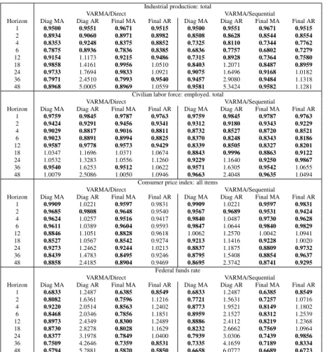
3.I RMSE relative to Direct AR(p) forecasts . . . . 80
3.II RMSE relative to ARMA(p,q) forecasts . . . . 82
3.III MSE of VARMA-based models relative to VAR-based forecasting factor model . . . 83
3.IV RMSE relative to Direct AR(p) forecasts . . . . 85
3.V RMSE relative to ARMA(p,q) forecasts . . . . 87
3.VI MSE of VARMA-based models relative to VAR-based forecasting factor model . . . 87
4.I Credit spreads . . . 103
4.II Explanatory power of global credit shock and common component 107 4.III Testing Granger causality between US and Canadian credit spreads 110 5.I Estimation of the number of factors in VAR time-varying coefficients127 5.II Summary of ML estimation of Factor-TVP VAR model . . . 137
I.II Variance decomposition and R2with monthly panel . . . xxxix
II.II Correlation between factors and variables in recursive identifica-tion in FAVAR-1 . . . xl II.IV Marginal contribution to R2in FAVAR-1 . . . . xli
II.VI Correlation between factors and variables in recursive identifica-tion in FAVAR-2 . . . xlii II.VIII Marginal contribution to R2in FAVAR-2 . . . xlii
xvii II.IX VAR models used to study effects and identification of financial
shock . . . xliv II.X Variance decomposition: contribution of the credit shock in SVAR
models . . . xlv III.I Results from simulation exercise 1, case 1 . . . liv III.II Results from simulation exercise 1, case 1, cont. . . lv III.III Results from simulation exercise 1, case 2 . . . lvi III.IV Results from simulation exercise 1, case 2, cont. . . lvii III.V Results from simulation exercise 2 . . . lviii
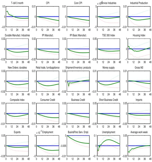
1.1 Impulse responses of some monthly indicators to national
mone-tary policy shock . . . 23
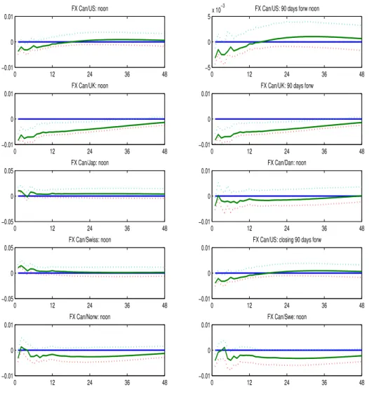
1.2 Impulse responses of exchange rates to national monetary policy shock . . . 24
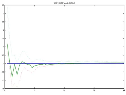
1.3 UIRP CAN/US, conditional on CA MP shock . . . 25
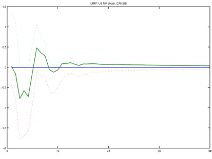
1.4 UIRP CAN/US, conditional on US Monetary policy shock . . . . 25
1.5 UIRP CAN/US, conditional on US MP or a global shock with al-ternative ordering . . . 26
1.6 UIRP CAN/US, conditional on US (global) credit shock . . . 26
1.7 FAVAR-VAR comparison. Here, VAR consists of [US Tbill, CPI, IP, CA Tbill, FX CA/US] . . . 27
1.8 Monthly estimates vs quarterly observed series . . . 28
1.9 Monthly estimates in annualized level . . . 28
2.1 Measures of the external finance premium . . . 39
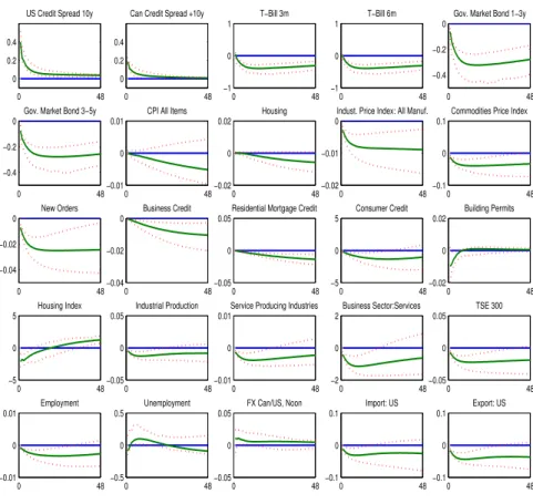
2.2 Dynamic responses of monthly variables to credit shock . . . 43
2.3 Dynamic responses of monthly variables to credit shock . . . 47
2.4 Dynamic responses of constructed monthly indicators to credit shock 48 2.5 Median IRFs of quarterly selected variables to credit shock . . . . 50
2.6 All IRFs satisfying sign restrictions . . . 51
2.7 Benchmark model, 100 basic points shock to credit spread . . . . 53
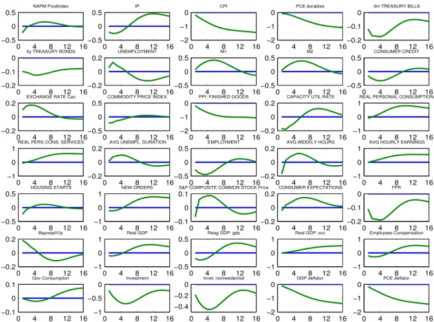
3.1 Comparison between FAVAR and FAVARMA-DMA impulse re-sponses . . . 89
3.2 FAVARMA-DMA impulse responses to monetary policy shock . . 90
4.1 Credit spreads used in identification of structural shocks . . . 104
4.2 Impulse of some variables of interest to one standard deviation global credit shock . . . 105
xix 4.3 Impulse of some variables of interest to one standard deviation
Canadian credit shock . . . 108 4.4 Comparison of impulse responses to a credit shock identified by
US and Canadian credit spreads . . . 109 5.1 Scree and trace tests for VAR model TVPs estimated by recursive
OLS . . . 127 5.2 Scatter plots for factor 1 and VAR model TVPs estimated by
re-cursive OLS . . . 128 5.3 Scatter plots for factor 2 and VAR model TVPs estimated by
re-cursive OLS . . . 129 5.4 Marginal contributions of factors to total R2on VAR model TVPs
estimated by recursive OLS . . . 130 5.5 Scree and trace tests for TVPs of VAR estimated by two-step
like-lihood method . . . 131 5.6 Scatter plots for factor 1 and TVPs of VAR estimated by two-step
likelihood method . . . 132 5.7 Scatter plots for factor 1 and VAR model TVPs estimated by
two-step likelihood method . . . 133 5.8 Common component and VAR model TVPs estimated by two-step
likelihood method . . . 134 5.9 Marginal contribution to total R2 of TVPs of VAR estimated by
two-step likelihood method . . . 135 5.10 Time-varying parameters from ML estimation of Factor-TVP VAR 136 5.11 Factor loadings from ML estimation of Factor-TVP VAR . . . 138 5.12 Marginal contribution to total R2 of TVPs and SVs of VAR
esti-mated by two-step likelihood method . . . 139 5.13 Marginal contributions of factors to total R2on VAR model TVPs
5.14 Time-varying parameters from ML estimation of Factor-TVP VAR with post-crisis data . . . 141 5.15 Factor loadings from ML estimation of Factor-TVP VAR with
post-crisis data . . . 142 I.1 Interest rates . . . xxiii I.2 Quarterly indicators IRFs to CA MP shock . . . xxiv I.3 Comparison of regional economic indicators relative to national
impulse responses . . . xxv I.4 Impulse responses of some quarterly indicators to identified
mon-etary policy shock . . . xxvii II.1 Principal components, rotated factors and variables used in
recur-sive identification with monthly balanced panel . . . xliii II.2 Principal components, rotated factors and variables used in
recur-sive identification with monthly mixed-frequencies data . . . xliv II.3 Benchmark model vs models 1-3, 100 basic points shock to credit
spread . . . xlv II.4 Dynamic responses of monthly variables to monetary policy shock xlvi II.5 Dynamic responses of monthly variables to monetary policy shock
using mixed-frequencies data . . . xlvii II.6 Dynamic responses of constructed monthly indicators to monetary
policy shock using mixed-frequencies data . . . xlvii IV.1 Regional impulse responses to a credit shock in deviation with
REMERCIEMENTS
L’accomplissement de ce travail aurait été impossible sans l’apport de plusieurs per-sonnes que je tiens à remercier ici. La liste n’est pas exhaustive et je m’excuse d’avance si tous ne sont pas cités.
Premièrement, je veux remercier mes deux directeurs de thèse, Jean-Marie Dufour et Jean Boivin, pour leur support continu et l’encadrement impeccable. Ils m’ont sagement transféré une partie de leur savoir-faire, autant en recherche qu’en enseignement, et je leur serai toujours reconnaissant.
Bien qu’il ne figure pas officiellement dans le comité de thèse, Marc Giannoni a été d’un grand support durant toutes ces années et nos nombreuses discussions ont grande-ment apporté à la complétion de ce travail.
Je remercie également Lynda Khalaf et Maral Kichian pour les innombrables discus-sions et encouragements ; Marine Carrasco et Benoît Perron pour le suivi et les commen-taires durant la rédaction de ma thèse ; ainsi que tout le corps professoral du département des sciences économiques de l’Université de Montréal pour les cours enseignés et com-mentaires sur mes recherches.
Un grand merci à Frank Diebold et Frank Schorfheide pour m’avoir invité au De-partment of Economics, de University of Pennsylvania, durant ma dernière année de doctorat. Ce fût une visite motivante et enrichissante.
Mon passage à l’Université de Montréal restera à toujours marqué par l’amitié déve-loppée avec les autres étudiants du programme de doctorat. Sans les nommer, cela pren-drait plusieurs pages, je veux souligner leur support, ouverture d’esprit, compétences et curiosité que j’ai eu la chance de découvrir au fil des années. Nos discussions intermi-nables vont certainement me manquer.
À tout le personnel du département des sciences économiques de l’Université de Montréal et celui du CIREQ ; merci pour leur dynamisme et leur efficacité.
Un grand merci tout particulier :
À mon épouse Claudia Gravel et notre fils Milan pour leur soutien quotidien dont ils ont fait preuve durant ces dernières années. Depuis son arrivée, Milan a été une source d’inspiration inattendue !
À mes parents Mitar Stevanovi´c et Nada Ivovi´c pour leur soutien inconditionnel depuis le premier jour de ma vie et pour leur décision courageuse de venir s’installer au Canada, en particulier à Québec, me donnant ainsi la chance d’un nouveau départ.
À Cezar pour sa fidèle compagnie.
Enfin, à mes collègues du département des sciences économiques de l’UQAM pour leur accueil convivial et leur support au début de ma nouvelle vie professionnelle.
INTRODUCTION GÉNÉRALE
Cette thèse est composée de cinq essais et s’inscrit dans le cadre des modèles à fac-teurs avec applications en macroéconomie. Les contributions empiriques sont : caracté-riser la transmission de la politique monétaire au Canada en corrigeant pour la plupart des anomalies répertoriées dans la littérature antérieure, identifier et quantifier, parmi les premiers, les chocs de crédit et leurs effets sur les économies américaine et canadienne, et produire la première évidence empirique sur la structure à facteurs des coefficients aléatoires dans les modèles macroéconomiques. Du point de vue théorique, une nouvelle classe de modèles est proposée et leur importance a été justifiée au niveau de la prévi-sion des agrégats macroéconomique et de l’analyse structurelle utilisant les fonctions de réponse impulsionnelles.
Le premier article analyse la transmission de la politique monétaire au Canada en utilisant le modèle vectoriel autorégressif augmenté par facteurs (FAVAR). Les études précédentes utilisant les modèles VAR structurels ont documenté plusieurs anomalies (price, exchange rate, delayed overshooting et uncovered interest rate parity puzzles), et les essaies de les corriger n’ont pas connu de grands succès. Puisque l’une des expli-cations des difficultés est le manque d’information dans les petits modèles empiriques, l’approche FAVAR est très attrayante car elle permet d’incorporer un très grand ensemble de données tout en ayant un modèle parcimonieux.
Le modèle est estimé avec un panel non balancé contenant 435 indicateurs écono-miques et financiers mensuels et trimestriels. Nous trouvons que l’information contenue dans les facteurs est importante pour bien identifier la transmission de la politique moné-taire dans les fréquences mensuelle et trimestrielle, et elle aide à corriger les anomalies empiriques présentes dans les modèles VAR. Finalement, le cadre d’analyse FAVAR permet d’obtenir les fonctions de réponse impulsionnelles pour tous les indicateurs dans l’ensemble de données, produisant ainsi l’analyse la plus complète à ce jour des effets de la politique monétaire au Canada.
L’objectif du deuxième article est d’examiner les effets et la propagation des chocs de crédit sur l’économie réelle en utilisant un grand ensemble d’indicateurs économiques
et financiers dans le cadre d’un modèle à facteurs structurel. Contrairement aux études précédentes, nous utilisons une procédure d’identification des chocs structurels moins restrictive avec pour but de laisser les réponses des taux d’intérêt et des indicateurs avancés complétement déterminées par les données. Le modèle est estimé en utilisant 187 indicateurs économiques et financiers américains.
Nous trouvons qu’un choc de crédit augmente immédiatement les credit spreads et cause une récession significative et persistante accompagnée d’une baisse considérable des niveaux des prix. De plus, les taux d’intérêt baissent significativement à l’impact ainsi que les indicateurs avancés tels que l’indice de marché immobilier, le sentiment des consommateurs, etc. Ces chocs ont un effet important sur des mesures d’activité réelle, indices de prix, indicateurs avancés et financiers. Contrairement aux autres études, notre procédure d’identification du choc structurel ne requiert pas de restrictions temporelles entre facteurs financiers et macroéconomiques. De plus, elle donne une interprétation des facteurs sans restreindre l’estimation de ceux-ci.
Dans le troisième article nous étudions la relation entre les représentations VARMA et factorielle des processus vectoriels stochastiques, et proposons une nouvelle classe de modèles VARMA augmentés par facteurs (FAVARMA). Notre point de départ est de constater qu’en général les séries multivariées et facteurs associés ne peuvent simultané-ment suivre un processus VAR d’ordre fini. Nous montrons que le processus dynamique des facteurs extraits comme combinaison linéaire des variables observées est en géné-ral un VARMA et non pas un VAR comme c’est supposé ailleurs dans la littérature. Deuxièmement, nous montrons que même si les facteurs suivent un VAR d’ordre fini, cela implique une représentation VARMA pour les séries observées. Alors, nous pro-posons le cadre d’analyse FAVARMA combinant ces deux méthodes de réduction de dimension.
Le modèle est appliquée dans deux exercices de prévision en utilisant des données américaines et canadiennes de Boivin, Giannoni et Stevanovi´c (2010, 2009) respective-ment. Les résultats montrent que la partie VARMA aide à mieux prévoir les importants agrégats macroéconomiques relativement aux modèles standards. Finalement, nous esti-mons les effets de choc monétaire en utilisant les données et le schéma d’identification
3 de Bernanke, Boivin et Eliasz (2005). Notre modèle parcimonieux FAVARMA(2,1) avec six facteurs donne les résultats cohérents et précis des effets et de la transmission moné-taire aux États-Unis. Contrairement au modèle FAVAR employé dans l’étude ultérieure où 510 coefficients VAR devaient être estimés, nous produisons les résultats semblables avec seulement 84 paramètres du processus dynamique des facteurs.
L’objectif du quatrième article est d’identifier et mesurer les effets des chocs de crédit au Canada dans un environnement riche en données. Dans le but d’incorporer l’informa-tion d’un grand ensemble d’indicateurs économiques et financiers, nous utilisons le mo-dèle FAVARMA structurel. Dans le cadre théorique de l’accélérateur financier développé par Bernanke, Gertler et Gilchrist (1999), nous approximons la prime de financement ex-térieur par les (credit spreads). Le modèle est estimé en utilisant les données mises à jour de Boivin, Giannoni et Stevanovic (2009).
D’un côté, nous trouvons qu’une augmentation non-anticipée de la prime de finan-cement extérieur aux États-Unis génère une récession significative et persistante au Ca-nada, accompagnée d’une hausse immédiate des credit spreads canadiens. La compo-sante commune semble capturer les dimensions importantes des fluctuations cycliques de l’économie canadienne. L’analyse par décomposition de la variance révèle que ce choc de crédit a un effet important sur différents secteurs d’activité réelle, indices de prix, indicateurs avancés et credit spreads. De l’autre côté, une hausse inattendue de la prime canadienne de financement extérieur ne cause pas d’effet significatif au Canada. Nous montrons que les effets des chocs de crédit au Canada sont essentiellement causés par les conditions globales, approximées ici par le marché américain. Finalement, étant donnée la procédure d’identification des chocs structurels, nous trouvons des facteurs interprétables économiquement.
Finalement, le dernier article innove en imposant une structure à facteurs au niveau des coefficients aléatoires d’un modèle empirique. Il est bien connu que le comporte-ment des agents et de l’environnecomporte-ment économiques peut varier à travers le temps (ex. changements de stratégies de la politique monétaire, volatilité de chocs) induisant de l’instabilité des paramètres dans les modèles en forme réduite. Les modèles à para-mètres variant dans le temps (TVP) standards supposent traditionnellement les processus
stochastiques indépendants pour tous les TVPs. Dans cet article nous montrons que le nombre de sources de variabilité temporelle des coefficients est probablement très petit, et nous produisons la première évidence empirique connue dans les modèles macroéco-nomiques empiriques.
L’approche Factor-TVP est appliquée dans le cadre d’un modèle TVP-VAR stan-dard. Nous trouvons qu’un seul facteur explique la majorité de la variabilité des coef-ficients VAR, tandis que les paramètres de la volatilité des chocs varient d’une façon indépendante. Le facteur commun est positivement corrélé avec le taux de chômage. La même analyse est faite avec les données incluant la récente crise financière. La procé-dure suggère maintenant deux facteurs et le comportement des coefficients présente un changement important depuis 2007. Finalement, la méthode est appliquée à un modèle TVP-FAVAR. Nous trouvons que seulement 5 facteurs dynamiques gouvernent l’insta-bilité temporelle dans presque 700 coefficients.
5 Contribution des coauteurs
Je suis le premier auteur de tous les cinq articles de cette thèse. Cependant, mes coauteurs Nathan Bedock, Jean Boivin, Jean- Marie Dufour, Marc Giannoni et moi-même contribuons à part égale.
Les deux premiers articles sont coécrits avec Jean Boivin et Marc Giannoni. Le troi-sième article est coécrit avec Jean-Marie Dufour et le quatrième avec Nathan Bedock.
MONETARY TRANSMISSION IN A SMALL OPEN ECONOMY: MORE DATA, FEWER PUZZLES
1.1 Introduction
Conclusions about the role that monetary policy plays in the economy and how it should be conducted in practice depend crucially on the way monetary policy affects the economy. This is why a large empirical literature has attempted to measure the transmission of monetary policy.
A standard approach to uncover the transmission of monetary policy is to use struc-tural vector autoregression (VAR). This method is particularly appealing since it does not require to specify complete model of the economy. It consists of imposing the minimum amount of restrictions needed to identify an exogenous source of variation in monetary policy, in a system of equations capturing the relevant macroeconomic dynamics, that is otherwise left unrestricted. Structural VAR methodology has been largely applied in both assessing the empirical fit of structural models and in policy applications. Some key examples of early and successful implementation on US data are Bernanke and Blinder (1992), Sims (1992), and Bernanke and Mihov (1998). Even if the identification strategy has been a source of disagreement (see Christiano, Eichenbaum and Evans (2000) for a survey), this simple method is still largely used, and delivers some useful information about the effects and the transmission of monetary policy shocks on economy.
However, for small open economies like Canada, uncovering the transmission mech-anism of monetary policy through this type of approach has proven to be an especially challenging task. In particular, initial VAR analysis on Canadian data have often doc-umented the presence of anomalies such as price, exchange rate, delayed overshooting and uncovered interest rate parity puzzles.
In Grilli and Roubini (1996) the authors used standard structural VAR model to eval-uate the effects of monetary policy shocks in two-country systems (the non-U.S. G-7
7 countries relative to the U.S.). Their results show strong evidence of several puzzles for most of non-U.S. countries. To solve some of these anomalies the authors replaced the short-term interest rate by the differential between short- and long-term interest rates in order to capture agents’ inflation expectations. The same anomalies are reported and re-solved in Kim and Roubini (2000) who used a structural VAR setup with non-recursive contemporaneous restrictions where the monetary policy shocks are identified by model-ing the monetary authority reaction function and the structure of the economy. Another alternative to simple recursive identification structure is to use some long-run proposi-tions of economic theory. For instance, Fung and Kasumovich (1998) estimate cointe-grated VAR models for G-6 countries and then identify monetary shocks by imposing the long-term money neutrality (a permanent change in the nominal stock of money has a proportionate effect on the price level with no long-run effect on real economic activity). In Cushman and Zha (1997) authors argue that puzzles found when estimating the effect of monetary policy shocks in small open countries are due to inappropriate identification schemes of monetary policy in such economies. Using Canada as benchmark case, they estimate a standard VAR model that contains two types of variables, domestic (CAN) and foreign (US), and impose block exogeneity condition on the latter. The monetary policy shock is identified by supposing that monetary authority observe immediately the exchange rate, interest rates, stock of money and world commodity price level. Using this nonrecursive identification they obtain impulse responses that are consistent with standard theory and highlight the exchange rate as a transmission mechanism. Finally, Bhuiyan and Lucas (2007) consider an alternative resolution of these puzzles based on an explicit account of inflation expectations. They first estimate ex-ante real interest rate and inflationary expectations by decomposing the nominal interest rate, and then include these into a fully recursive VAR model to evaluate the effects of monetary policy shocks. Their findings suggest more broadly, that the anomalies reported above might be the result of omitted information from small-scale VARs.
Hence, it is particularly interesting to see if a more systematic use of the relevant information available could yield a more coherent and accurate picture of the effect of monetary policy in a small open economy. In this paper, we use a factor augmented
vector autoregression (FAVAR) approach to assess the effect and transmission mecha-nism of monetary policy shocks on economic activity in Canada1. Given that a common potential explanation of all difficulties reported above is the lack of information in small-scale VAR models, the FAVAR approach is appealing in a priori since it incorporates a huge amount of information in a parsimonious way. Moreover, the application to U.S. data by Bernanke, Boivin and Eliasz (2005) was a success story.
In our implementation, we estimate the FAVAR model using an unbalanced data set of 348 monthly and 87 quarterly macroeconomic Canadian time series. We find that the information summarized by the factors is important to properly identify the monetary transmission mechanism in both monthly and quarterly frequencies. Overall, our benchmark FAVAR specification, that includes only the monetary policy instrument as observed factor, leads to broadly plausible estimates of the effects of monetary policy shocks on many macroeconomic variables of interest and contributes to mitigate puzzles mentioned above. Indeed, all price indexes decline after an unexpected increase in short rate while the exchange rates appreciate on impact.
When comparing to standard small open economy VAR model results, we find that adding information through factors into this VAR corrects for price and exchange rate puzzles, and for inconsistent response of industrial production with respect to long-run money neutrality. Also, the maximum response of exchange rates is on impact which corrects for delayed overshooting puzzle. Finally, we find no evidence of the uncov-ered interest rate parity, meaning that there is no systematic carry trade conditional on a domestic monetary policy shock that rises the domestic interest rate.
Relative to existing literature discussed above, our approach is able to uncover rea-sonably the monetary policy transmission in a small open economy without searching to include agents’ expectations measures or other theoretical concepts proxies, and using the simplest recursive identification scheme. Moreover, the FAVAR framework allows us to check impulse responses for all series in the informational data set, and thus pro-vide, to our knowledge, the most comprehensive picture to date of the effect of Canadian
1. In independent research projects, Mumtaz and Surico (2009), and Forni and Gambetti (2010), obtain similar results for some of the puzzles that we study in this paper.
9 monetary policy.
The rest of the paper is organized as follows. The FAVAR methodology is detailed in the following section. In Section 3 we explain our application by presenting data and the strategy to identify the monetary policy shocks. The main results are presented and discussed in Section 4, and we conclude in Section 5.
1.2 FAVAR: Motivation, Methodology and Estimation 1.2.1 Motivation
Since Bernanke and Blinder (1992) and Sims (1992), the structural analysis applied macroeconomics employs vector autoregressive (VAR) models to identify and measure the effects of different shocks on macroeconomic variables of interest. Typically, cen-tral banks are interested in the behavior of macroeconomic aggregates after a monetary policy shock, and their analysts use widely structural VARs in order to identify the inno-vation. Several criticisms of the VAR approach are worth of noting. The most important is that it uses only a small number of variables to conserve degrees of freedom. This small number of variables is unlikely to span the information sets used by actual central banks that follow a large number of data series. Then, the lack of information leads to three big potential problems. First, the identification of shock can be contaminated which leads to several "puzzles" observed in the literature. Grilli and Rubini (1996) paper offers a nice overview of puzzles found in several papers:
– The price puzzle. When monetary policy shocks are identified with innovations in interest rates, the output and money supply responses are correct as a contrac-tionary increase in interest rate is associated with a fall in the money supply and the level of economic activity. However, the response of the price level is a persistent increase rather than a decrease.
– The Exchange rate puzzle. While a positive innovation in interest rates in the US is associated with an impact appreciation of the US dollar relative to the other G-7 countries, such monetary contractions in other G-7 countries are often associated with an impact depreciation of their currency value relative to the US dollar.
– The forward discount bias puzzle If uncovered interest parity holds, a positive in-novation in domestic interest rates relative to a foreign ones should be associated with a persistent depreciation of the domestic currency after the impact apprecia-tion, as the positive interest rate differential leads to an expected depreciation of the currency. However, the data show that a positive interest differential is associ-ated with a persistent appreciation of the domestic currency for periods up to two years after the initial monetary policy shock.
Further problem implied by lack of information in small-scale VAR models is the omitted variable problem. If important variables are not included in the system (corre-lated with regressors in the model) this leads to biased estimates of VAR coefficients which is likely to produce biased impulse responses worthless for structural analysis. The typical example in the literature is the omission of commodity prices in structural VAR analysis attempting to measure monetary policy in U.S. (see Sims (1992) for ex-planation).
The second problem in small-scale VAR model is that the choice of a specific data series to represent a general economic concept is arbitrary. Moreover, measurement er-rors, aggregation and revisions pose additional problems for linking theoretical concepts to specific data series. Finally, even if the two previous problems do not occur, i.e. a small scale VAR is well defined and the shock is well identified, we can produce im-pulse responses only for variables included in the VAR.
On the other side, a factor-augmented VAR, which will be discussed deeply in the next section, is a way to introduce additional information and then overcome the previ-ous discussion. It uses a simply dimension reduction with principal components analysis, which permits to resume a big part of information contained in a huge panel, into small number of factors. In the case of the monetary policy studies where the monetary policy instruments is an interest rate, Bernanke, Boivin and Eliasz (2005) show that including only 3 factors correct the price puzzle while keeping a low-dimensional estimated VAR and the easiest identification scheme. Finally, we can compute the impulse response functions for any variable in the informational panel which can be very important if the central bank is interested for example into the behavior of several price indices instead
11 in a total consumer price index only.
1.2.2 Methodology
We apply the Factor Augmented Vector Autoregressive (FAVAR) approach as in Bernanke, Boivin and Eliasz (2005), or BBE for the rest of the paper. Consider a T × M matrix of observable economic series Y , where T is the time size (number of periods) and M is the cross-sectional size (number of series). In the standard VAR (and struc-tural VAR) models used in monetary literature, Y include several variables assumed to drive the dynamics of the economy and the transmission of monetary policy shocks. The usual candidates are some measures of economic activity (GDP, industrial production, employment, unemployment rate, etc.), an indicator of price level (usually CPI), and a policy instrument (e.g. Federal Funds Rate (FFR) in US, Overnight rate in Canada, Monetary base, etc.). In the traditional (S)VAR approach, Y is modeled alone assuming that all relevant information is contained in several lagged values of Y . However, ad-ditional information available in other economic series may be relevant to the dynamic relationships assumed in VAR model, and this lack of information can lead to some unanticipated implications from the estimated model as pointed out in the previous sec-tion.
If this additional information can be summarized by a T × K unobserved factors matrix F, where K is relatively small, we can augment the standard VAR model by adding the factors. As illustrated by an example in BBE, the factors can be seen as proxies for the economic activity, price pressures, credit conditions or other theoretical concepts that are difficult to identify by one or two variables.
Suppose that the joint dynamics of (Ft,Yt) can be represented by the following
Ft Yt = Φ (L) Ft−1 Yt−1 + νt (1.1) = φf f(L) φf y(L) φy f(L) φyy(L) Ft−1 Yt−1 + et
where Φ(L) is the usual lag polynomial of finite order p, and νt is the error term with
mean zero and covariance matrix Q. It is easy to see that (1.1) becomes a standard VAR in Yt if the matrix Φ(L) is diagonal, i.e. if all terms in φf y(L) and φy f(L) are zero
(implying that there is no direct Granger causal relation between Ft and Yt). Otherwise,
the system (1.1) is defined as a factor augmented vector autoregression (FAVAR). It is important to notice that since FAVAR nests VAR representation in Yt, estimating
the former allows us to evaluate the marginal contribution of factors by comparing the results with existing VAR analysis. If the best approximation (in reduced form) of the true DGP (data generated process) is a FAVAR, then omitting Ft from (1.1) and
esti-mating the VAR model will lead to biased estimates of the VAR coefficients. Thus, the structural interpretations of the impulse responses are worthless.
If the factors Ft were observed, equation (1.1) would be a standard VAR model and
we would use existing structural VAR techniques to estimate the model and identify structural shocks. Unfortunately, Ft are unobservable and we have to learn something
about them from the relevant and available economic time series. Suppose that we have a panel of observable and informative economic series contained in a N × 1 vector Xt.
The number of series, N, can be arbitrary large relatively to the time series size T , but assumed to be much larger than the number of factors in Ft, K, and observed variables in
Yt, M. Then, we need to assume a relation between our observable series and the factors
that we need to estimate. The relation is given in the following observation equation:
13 where Xt is an (Nx1) vector of informative time series, Λf is an (NxK) matrix of factor
loadings, Λy is an (NxM) matrix of loadings relating the observable factors in Y t to Xt,
and ut is the (Nx1) vector of error terms. The errors are of mean zero and can display a
small amount of cross-correlation. Note that (1.2) states that both Ft and Yt explain the
dynamics of Xt. Thus, if we condition the statement on Yt, we can interpret Xt as noisy
measures of the underlying unobserved factors Ft.
Hence, defining Ft = [Ft′ Yt′]′ and Λ = [Λf Λy] the FAVAR model can be
repre-sented in an approximate static factor model form:
Xt = ΛFt+ ut (1.3)
Ft = Φ(L)Ft−1+ et (1.4)
where approximate stands for allowing some weak cross-section and time dependence among idiosyncratic components in et, and where Ft contains both observed and
un-observed factors. Note that considering a static version, i.e. (1.2) doesn’t contain any lagged values of Ft or Yt, is not a big constraint since dynamic factor model can always
be written in a static form.
1.2.3 Estimation
Recall from the previous section that the estimation of the model in (1.1) would be trivial if the factors were observable. Since this is not the case, we have to estimate them from Xt.
The unknown coefficients in (1.3)-(1.4) can be estimated by Gaussian maximum likelihood (or by Quasi ML) using the Kalman filter, see Engle and Watson (1981), Stock and Watson (1989), Sargent (1989). This method is computationally burdensome when N is very large, but also the misspecification becomes very likely.2
Instead of the likelihood-based approach, we use the two-step Principal Component
2. However, there are some recent improvements: Kalman filter speedup by Jungbacker and Koopman (2008), using principal components as very good starting values then a single pass of the Kalman filter by Giannone, Reichlin, and Sala (2004), and principal components for starting values then use EM algorithm to convergence by Doz, Giannone, and Reichlin (2006).
Analysis (PCA) estimation method.3 It is a non-parametric way to uncover the common space spanned by the factors of Xt, denoted by C(Ft,Yt). In the first step, the equation
(1.2) is considered. The space spanned by the factors is estimated by the first K+M principal components of Xt, and is denoted by ˆC(Ft,Yt). One should note that estimating
factors in this way is not the most efficient method since we do not exploit the fact that
Yt is observed. However, Stock and Watson (2002a) show that if N is large and the
number of principal components is at least as large as the true number of factors, the principal components consistently recover the space spanned by both Ft and Yt. In that
case, we need to identify the part of ˆC(Ft,Yt) that is not spanned by Yt in order to obtain
the estimate of Ft, ˆFt. This task depends on identification imposed in the second step
where the equation (1.2) is estimated by standard methods since unobserved factors are replaced by ˆFt. In the second step, the factors’ dynamic process is approximated by
standard finite order VAR.
The principal components approach is easy to implement and do not require very strong distributional assumptions. However, since the unobserved factors are estimated and then included as regressors in FAVAR model, the two-step approach suffers from the "generated regressors" problem. In order to get the accurate statistical inference on the impulse response functions, we use a bootstrap procedure proposed by Kilian (1998) that accounts for the uncertainty in the factor estimation.
1.3 Application
The purpose of this paper is to study the dynamic effects of monetary policy shocks on a variety of economic variables in Canada. We previously pointed out some problems with (S)VAR models and we discuss in this section how FAVAR model can deal with some of them.
Since the FAVAR approach consists of adding to a standard VAR K common com-ponents from a large number of relevant economic variables, it should deal with the lack of information problem in traditional (S)VAR literature. Moreover, we showed above
3. See Stock and Watson (2002a), and Bai and Ng (2006) for theoretical results concerning the PCA estimator.
15 that the system (1.1)-(1.2) nests the VAR specification. Then, it is possible to discuss directly if the marginal information brought by estimated factors is relevant or not. An-other problem that FAVAR approach can avoid is to assume that theoretical concepts such as real economic activity or price pressure are observed. Also, this approach allows us to study the dynamic responses to monetary policy shock of all variables in Xt, not
only in Yt. Finally, Forni et al. (2009) argues that while non-fundamentalness is generic
of small scale model, they cannot arise in a large dimensional dynamic factor models4. This is of primary importance since the objective is to identify a relatively new structural shock in empirical macroeconomics.
Let us state now the FAVAR and VAR models that will be used to assess the effect of monetary policy shocks in Canada. The benchmark model is a FAVAR where Yt contains
only one variable, the monetary policy instrument, and Ft contains K unobserved factors.
The official monetary policy instrument of the Bank of Canada is the overnight rate. Since this variable is available only from 1975M1, and our application uses data from 1969M1, we take the 3-month Treasury Bill (T-bill) as a proxy5. In order to discuss the
additional information brought by the factors, we will compare a standard VAR model, where Y contains Industrial production (IP), Consumer price index (CPI), T-Bill and CAN/US Exchange rate (FX-CAN/US), with FAVAR models where Y is augmented by a number of estimated factors.
1.3.1 Data
We estimate the system (1.1)-(1.2) with Canadian data used in Gosselin and Tkacz (2001) and updated with some variables from Galbraith and Tkacz (2007). There are 348 monthly series starting from 1969M1 and ending on 2008M6, and 87 quarterly series covering 1969Q1-2008Q2 time period. These series are initially transformed to induce stationarity. The description of the variables in the data set and their transformation is given in Appendix. To use the two-step approach, we need a balanced panel. Then,
4. If the shocks in the VAR model are fundamental, then the dynamic effects implied by the moving average representation can have a meaningful interpretation, i.e. the structural shocks can be recovered from current and past values of observable series.
if we wish to use all available information, we have to mix both monthly and quarterly panels. Hence, we need to replace missing values when transforming the quarterly series to monthly indicators. Moreover, several monthly series contain missing values. To face these irregularities and obtain a balanced data set, we apply the EM algorithm proposed by Stock and Watson (2002b)6.
Before discussing the estimation results, we need to specify the identification restric-tions in the two-step approach, and how the monetary policy instrument is imposed as an observable factor.
1.3.2 Identification in the two-step approach
Different sets of identification restrictions must be imposed before estimating the system (1.1)-(1.2). The first consists of normalization restrictions on the observation equation (1.2) because of the fundamental indeterminacy of this model. Suppose that ˆΛ and ˆFt are a solution to the estimation problem. However, this solution is not unique
since we could define ˜Λ = ˆΛH and ˜Ft= H−1Fˆt, where H is a K × K nonsingular matrix,
which could also satisfy equation (1.2). Then, observing Xt is not enough to distinguish
between these two solutions, and a normalization is necessary. We use the standard normalization in the principal components approach, that is, we take C′C/T = I, where
C= [C(F1,Y1), ...,C(FT,YT)]. Then, ˆC=
√
T ˆZ, where ˆZ are the eigenvectors
correspond-ing to the K largest eigenvalues of XX′, sorted in descending order.
The second identification issue is to identify the structural shocks in equation (1.1). As in most VAR model applications in the monetary policy literature, we adopt a recur-sive structure where the monetary policy instrument is ordered last in Yt (all the factors
6. The choice of data to include in Xt is not obvious. Theoretically, more data (and that means larger time size, T ↑, and more series, N ↑) is better because the estimators in two-step approach are asymptotically consistent and the asymptotic theory here has two dimensions, T and N. But in practice,
T is maximized with data availability constraint while augmenting N (and adding relevant information)
means more of the same type data (e.g. CPI category has dozens of subcategories). Boivin and Ng (2006) provide examples where adding more data has perverse effects in forecast exercise. The idea is that while the two-step estimators are consistent even in presence of weak cross-correlation between the errors in (1.3), adding many data of the same type in the finite sample context could increase the amount of cross-correlations in the error term and alter the performance of the PCA estimator. However, the pre-screening proposed by Boivin and Ng (2003) is largely ad hoc, and the cost from using all series, if any, is marginal in practice.
17 entering (1.1) respond with a lag to a monetary policy shock). In that case, we don’t need to identify the factors separately, but only the space spanned by the latent factors,
Ft.
Recall that in the first step, relying on the fact that when N is large, the principal components estimated from Xt, ˆC(Ft,Yt), consistently recover K+M independent, but
arbitrary, linear combinations of Ft and Yt. Since Yt is not explicitly imposed as a factor
in the first step, any of the linear combinations underlying ˆC(Ft,Yt) could involve the
monetary policy instrument, which is always ordered last in Yt. Then, it would not be
valid to simply estimate a VAR in estimated factors from entire data set and Yt, and use
the recursive policy shock identification framework. In that case, we need to remove the direct dependance of ˆC(Ft,Yt) on Yt, where Yt is T-bill. If linear combinations of Ft and
Yt were known, this would involve subtracting Yt times the associated coefficient from
each of the elements of ˆC(Ft,Yt).
Since these are unknown, to impose Yt as a factor in the first step we use the iterative
principal components approach as in Boivin and Giannoni (2007). Starting from an initial estimate of Ft, Ft0:
1. Regress Xt on Ft0and Yt, to obtain ˆλ 0 t 2. Compute ˜Xt0= Xt− ˆλ 0 tYt 3. Estimate F1
t as the first K-1 principal components from ˜Xt0
4. Back to 1.
Contrary to BBE’s strategy, it does not rely on any temporal assumption between the observed factors and the informational panel. Hence it can be used for any set of observed factors without imposing any further assumptions. We adopt this approach in our exercise with setting the number of iterations at 157.
1.4 Results
One interesting feature of the FAVAR approach is that we can produce impulse re-sponses for all observable series (in both informational panel and observed factors).
Hence, we can explore the reaction of the economy to a structural shock on a much broader set of dimensions than in the case of small-scale VAR models. Given our mixed-frequencies approach, we can also conduct the exercise at both monthly and quarterly frequencies.
1.4.1 Effects of a monetary policy shock
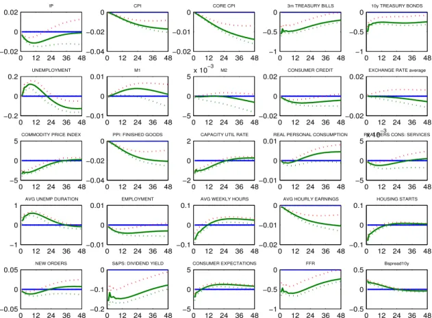
Here, we discuss results using mixed-frequencies monthly panel where the bench-mark model contains 8 unobserved factors and one observed factor, T-Bill. Figure 1.1 contains impulse response for some economic indicators of interest to a monetary policy shock8. We can see that a positive shock on the T-Bill implies a persistent economic slowdown. The production indicators go down progressively, and price indexes present a very persistent decreasing reaction. The leading economic indicators such as housing index, new orders and retail trade, and money aggregates decline significatively. Overall, these results seem to provide a consistent measure of the effect of monetary policy in a small open economy.
The impulse responses of several exchange rates are presented in Figure 1.2. We can see that Canadian dollar appreciates in most of the cases, and especially with respect to the US dollar, meaning that there is no evidence of exchange rate puzzle. Moreover, the maximum response is on the impact, so the delayed overshooting puzzle is corrected too. The impulse responses of interest rates are presented in Figure I.1. They jump initially above the steady state and eventually go down.
Since we have constructed a mixed-frequencies monthly panel, we can produce monthly impulse responses of economic indicators observed only at quarterly frequency. In Figure I.2, in Appendix, we plot impulse responses of some of these constructed monthly indicators. We can see a significative decline in GDP components. Moreover, it is interesting to see if there are some differences in the response to monetary policy shock across different regions in Canada. To do so we grouped some available series of interest in fours regions: Atlantic, Center, Prairie and BC. In Figure I.3 we plot their re-sponses in deviation to the response of corresponding national variable. We can see that
19 Atlantic, Center and BC regions present quite similar pattern while the Prairie provinces seem to diverge from the other provinces.
The Table I.II in Appendix presents variance decomposition and R2 results. The
first column reports the contribution of the monetary policy shock to the variance of the forecast error at four year horizon, and the second column contains the R2 of the common components for 80 variables of interest. As in BBE paper, we find that the monetary policy shock has a small effect on most of the variables, except for interest rates and money supply. Looking at the R2results we conclude that the common component explains an important fraction of variability in observable series, meaning that extracted factors do capture important dimensions of the business cycle movements.
1.4.2 Uncovered interest rate parity puzzle
The UIRP puzzle has been a very challenging task in the standard VAR framework. Including the information through factors seems to help in resolving this issue. We construct a measure of the forward discount premium following Scholl and Uhlig (2005). Let ikand i∗kbe domestic and foreign interest rates impulse responses at horizon k. Define
s0and skas impulse responses of the log of the exchange rate at the impact and at horizon
krespectively. The UIRP measure (or the forward discount premium) is calculated as:
U IRP= (ik− i∗k) + (sk− s0).
In Figure 1.3, we plot the impulse response function for the UIRP between Canada and US, calculated for 3-month Treasury bills. Surprisingly, conditional on the domestic monetary policy shock, there is no carry trade on the impact. However, the confidence intervals are quite large. After a year, the response is close to zero.
In Figure 1.4, we plot the impulse responses of the same measure but after the US monetary policy shock. It is identified recursively by including the US 3-month T-bill first in the VAR ordering. In that case, the UIRP measure is significatively different from zero on impact. However, we do not interpret this as a violation of the uncovered interest parity hypothesis since the US monetary policy shock is understood as proxy for a global