ELEMENTS OF THE METACOMMUNITY STRUCTURE: COMPARlSON ACROSS MULTIPLE METACOMMUNITIES
THESIS PRESENTED
AS A PARTIAL REQUIREMENT FOR THE MASTER IN BIOLOGY
BY
RENATO HENRIQUES DA SILVA
UNIVERSITÉ DU QUÉBEC À MONTRÉAL Service des bibliothèques
Avertissement
La diffusion de ce mémoire se fait dans le respect des droits de son auteur, qui a signé le formulaire Autorisation de reproduire et de diffuser un travail de recherche de cycles supérieurs (SDU-522 - Rév.01-2006). Cette autorisation stipule que «conformément
à
l'article 11 du Règlement no 8 des études de cycles supérieurs, [l'auteur] concède àl'Université du Québec à Montréal une licence non exclusive d'utilisation et de publication oe la totalité ou d'une partie importante de [son] travail de recherche pour des fins pédagogiques et non commerciales. Plus précisément, [l'auteur] autorise "Université du Québec à Montréal à reproduire, diffuser, prêter, distribuer ou vendre des copies de [son] travail de recherche à des fins non commerciales sur quelque support que ce soit, y compris l'Internet. Cette licence et cette autorisation n'entraînent pas une renonciation de [la] part [de l'auteur] à [ses] droits moraux ni à [ses] droits de propriété intellectuelle. Sauf ententé contraire, [l'auteur] conserve la liberté de diffuser et de commercialiser ou non ce travail dont [il] possède un exemplaire.»
ÉLÉMENTS DE LA STRUCTURE D'UNE METACOMMUNAUTÉ:
COMPARAISON
À
TRAVERS MULTIPLE METACOMMUMAUTÉSMÉMOIRE PRESENTÉ
COMME EXIGENCE PARTIELLE DE LA MAÎTRISE EN BIOLOGIE
PAR
RENATO HENRIQUES DA SILVA
ACKNOWLEDGEMENTS
l first want to thank my research advisor, Pedro R. Peres-Neto, Ph. D., professor at Université du Québec à Montréal (UQAM), for the opportunity he provided me, as weil as for aIl his patience, advices and trust in me throughout the masters program. His training and methods were fundamental for my achievements in academia and in life. l would also like to thank Sapna Sharma, Ph. D., and Tariq Gardezi, Ph. D., for providing the data that allowed the feasibility of the project and Mélanie Desrochers for her help with GIS. A thank you to the members of my committee, Beatrix Beisner, Ph. D., and Christian Messier, Ph. D., for their valuable advices and critiques on the present work. l want to specially thank Bailey Jacobson, for ail her help, in many ways, in my project, and for her friendship, as weil as the other students for ail their support: Rich Vogt, Daniel Pires, Caroline Senay, Mehdi Layeghifard, Joachim Prunier, Marie Christine Bellemare and Aline Aguiar. Thank you to ail the UQAM employees for their help. l wou Id like to thank my father, Durval Henriques da Silva Filho and the l'est of my family for their support, which was crucial to my success. A special thanks goes to my wife Monique Ariane Rezende Henriques da Silva for her patience and love. Finally, l would like to acknowledge the Natural Sciences and Engineering Research Council of Canada (NSERC), which provided financial support for this project.
RÉSUMÉ Xv
INTRODUCTION
ABSTRACT xiii
1.1 State of knowledge
1.2 Study system 2
1.3 Community Ecology and the metacommunity paradigm 4
1.4 Elements of Metacommunity Structure (EMS) 6
1.5 The phylogenetic structure of ecological communities 13
CHAPTERI
A COMMUNITY OF METACOMMUNITIES: EXPLORING PATTERNS IN
SPECIES DISTRIBUTION ACROSS LARGE GEOGRAPHIC AREAS 19
2.1 Introduction 20
2.1.1 Metacommunities: Structural versus Mechanistic approach 20 2.1.2 Patterns of distribution and the Elements of Metacommunity 21 Structure
2.1.3 Looking further into EMS framework 23
2.1.4 Lake-fish systems as metacommunities 24
vi
2.2 Methodology 25
2.2.1 Ontario Fish Distribution Database (OFDD) 25
2.2.2 Lake Inventory Database (LINV) 25
2.2.3 Species used in the analysis 26
2.2.4 Watershed as metacommunities 26
2.2.5 Statistical Analyses 27
2.2.5.1 Ordination 27
2.2.5.2 Nul! model 28
2.2.5.3 EMS analyses 29
2.2.6 Biotic and abiotic lake indices 31
2.2.6.1 Community similarity 31
2.2.6.2 Watershed connectivity 32
2.2.6.3 Postgladal dispersal 32
2.2.6.4 Environmental gradient length 33
2.2.6.5 Abiotic integration 33
2.2.7 Environmental versus spatial variation 34
2.3 Results 35
2.3.1 Environmental and spatial drivers of metacommunity patterns 35
2.3.2 Species turnover at the Provincial scale 42
2.4 Discussion 45
2.4.1 Nestedness versus Clementsian gradient 45
2.4.2 Large-scale patterns 49
CHAPTER II
COMMUNITY PHYLOGENETIC STRUCTURE AND SPECIES NICHE:
3.1 Introduction 52
3.1.1 Why use patterns of distributions? 52
3.1.2 Influence of niche on distributional patterns 53 3.1.3 Phylogenetic relatedness and community assembly 54 3.1.4 Integrating phylogeny and niche into metacommunity patterns 54
3.1.5 Studied system 55
3.1.6 Chapter objectives 56
3.2 Methodology 56
3.2.1 Niche indices 56
3.2.2 Characterizing environmental gradients 58
3.2.3 Phylogenetic tree 58
3.2.4 Phylogenetic indices 60
3.2.5 Nul! model for phylogenetic data 60
3.2.5.1 Regional null model 60
3.2.5.2 Local nul! model 61
3.2.6 Statistical analyses 65
3.2.6.1 Provincial scale patterns - Relation between environmental
gradients and indices 65
3.2.6.2 Provincial scale patterns - Variation in phylogenetic
structure, community niche structure and environment across watersheds 65 3.2.6.3 Watershed scale patterns - Differences in species and
environ mental properties between metacommunity patterns 67
3.3 Results 67
3.3.1 Regional and local null models 67
3.3.2 Environmental gradients, phylogenetic structure and community
viii
3.3.3 Differences between nestedness and Clementsian gradients
regarding indices 76
3.4 Discussion 77
3.4.1 Regional and local filters 77
3.4.2 Differences between rnetacornrnunity distributional patterns 81
3.4.3 Linking environrnental gradients to corn munity phylogenetic
structure and species niches 82
CONCLUSION 87
corresponding codes from Table 1.1. Watersheds without codes have no data available. Map adapted from Ministry of the
Environment (2004). Il
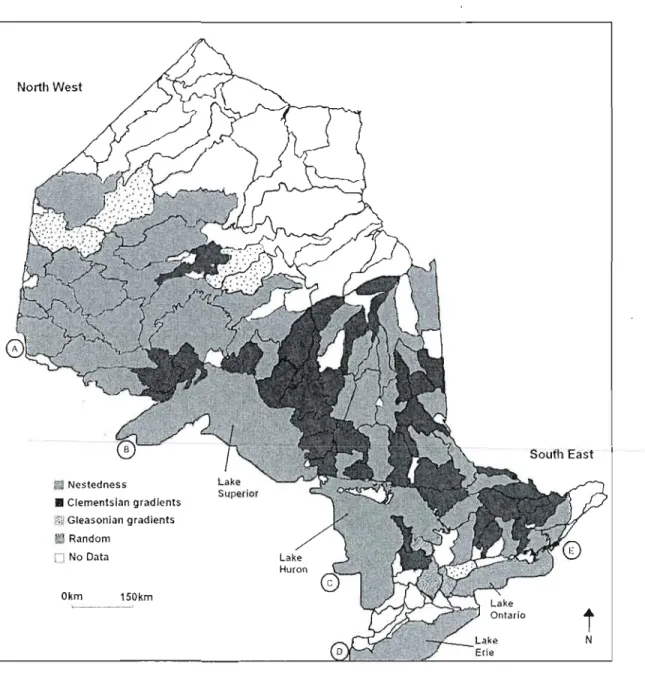
1.2 General framework for the Elements of Metacommunity Structure (coherence, turnover and boundary clumping). Columns represent sites and rows represent species. NS == non significant. See Table 1.2 for EMS results of the hypothetical matrices. 14 2.1 EMS results on Ontario tertiary watersheds. Map modified from
Miriistry of Environment (2004). The letters refers to postglacial dispersal routes. A == Glacial Lake Agassiz; B == Brule-Portage Outlet; C == Grand Valley Outlet; D == Fort Wayne; E == Champlain Outlet (Mandrak & Crossman, 1992b).
38
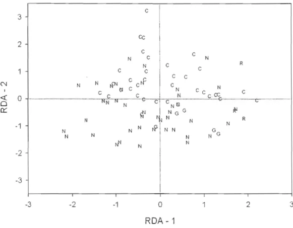
2.2 Redundancy analysis on Elements of metacommunity structure (coherence, turnover and boundary c!umping) standardized values. Score coordinates of each metacommunity according to axes. N ==
nestedness, C == Clementsian gradients, G == Gleasonian gradients and R == random.
39
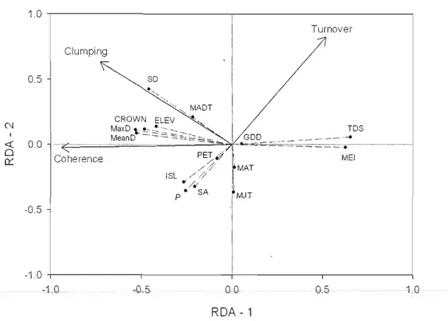
2.3 Redundancy analysis from EMS and correlations with environmental variables. Solid lines with arrows represent the EMS. Dashed lines with small circles represent the environmental variables. SA ==
surface area, P == shoreline perimeter, lSL == island perimeter, SD == secchi depth, MaxD == maximum depth, MeanD == mean depth, CROWN == crown canopy coyer, ELEV == elevatlon, GDD ==
growing degree-days, TDS == total dissolved solids, MEl == morpho
edaphic index, MADT == mean annual daily temperature, MIT ==
mean July temperature, MAT == mean August temperature and PET
== potential evapotranspiration. 40
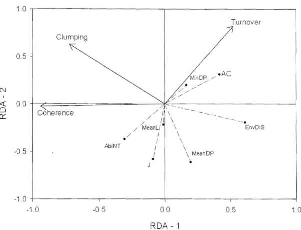
2.4 Redundancy analysis from EMS and correlations with indices. Solid lines with arrows represent the EMS. Dashed lines with small circles represent indices. MeanL == mean latitude, AC == average connectivity, AbINT == abiotic integration, EnvDis == environmental distance, J == Jaccard index, MlnDP == minimal distance from postglacial route and MeanDP == mean distance from postglacial
x
Figure Page
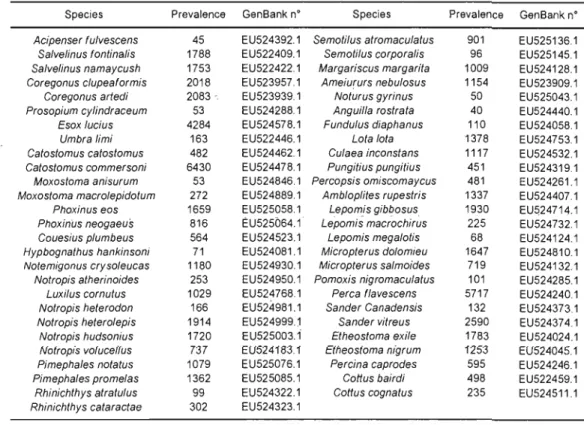
3.1 Phylogenetic tree of the 53 extant species created using mid-point rooted Neighbour-joining tree technique (Saitou & Nei, 1987) applied on K2P distances (Kimura, 1980) Prevalence = number of
lakes where the species is present. 63
3.2 Conceptual framework for the regional and local null models, which represent the filters that species need to surpass in order to assemble in local communities. The regional filter represents broad-scale factors (e.g., climate variables and/or dispersal limitation such as geographic barrier). The local filter represents local dispersal limitation (e.g., community isolation), local environment (e.g., pH) and/or biotic interactions (e.g., competition). Species are represented by symbols. "Under" stands for underdispersion (i.e., phylogenetic clustering), "Over" stands for phylogenetic overdispersion (i.e., phylogenetic evenness) and "Random" stands for random
phylogenetic structure. 68
3.3 Results from ANOVAs on environmental gradients indices between the two main metacommunity patterns (nestedness and Clementsian
gradient). The a-Ievel used was 0.05. 78
3.4 Results from ANOVAs on watershed phylogenetic and niche indices between the two main metacommunity patterns (nestedness and Clementsian gradient). The a-level used was 0.05. 79
Abbreviations as outlined on Ontario map of Figure 1.1.
page 4. Watersheds are presented in 7 1.2 Results of EMS analyses on hypothetical matrices from Figure 1.2.
Analyses were performed using the first ordination axis extracted via reciprocal averaging and based on community perspective. Abs = number of embedded absences; Re = number of replacements; Mo = Morisita's index; l! = mean value of each element for the random distribution; cr = standard deviation of each element for the random
distribution; p = significance probability; SV = standardized value. Significant results (p :::; 0.05) are in bold. *Coherence standardized values were multiplied by -1. ** Mo is statistically tested with a two-tailed test, thus when p 2. 0.95, the result is significant and indicate an evenly-spaced gradient pattern.
15
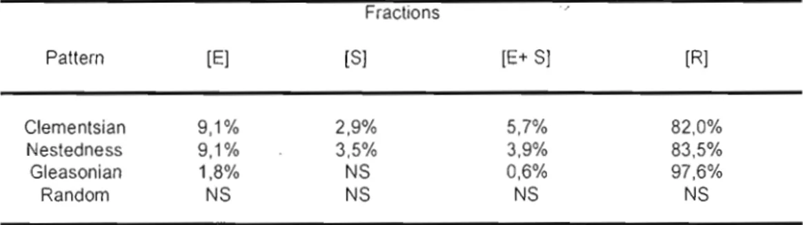
2.1 Results for variation partitioning. Values presented are the average values for ail watersheds within each pattern. [E] = the fraction of variation explained solely by the environment; [S] = the unique fraction of variation explained by space; [E+S] = the corn mon fraction of the variation shared by space and environment; [R] = residual variation.
43
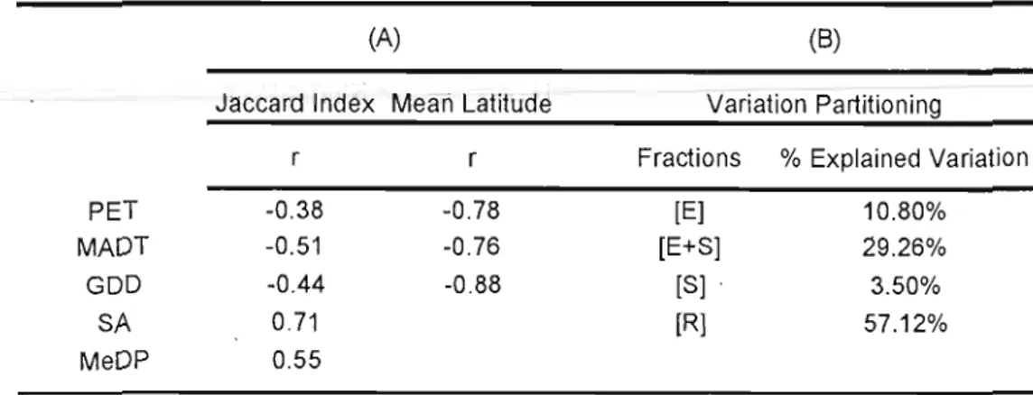
2.2 Results for "selective colonization" and "species turnover at the provincial scale" sections. (A) Pearson correlations. PET = potential evapotranspiration; MADT = mean annual daily temperature; GDD = growing degree days; SA = surface area; MeanDP = mean distance from postglacial routes. All correlations in the table are significant (p < 0.05); r = correlation coefficient. (B) Results for variation particioning across watersheds. Ali fractions are significant
(p < 0.05). [E] = the unique fraction of variation explained by the environment; (S] = the unique fraction of variation explained by space; [E+S] =the corn mon fraction of the variation shared by space and environment; and [R] = residual variation. 44
xii
Table Page
3.1 Species name, prevalence (number of lakes present) and GenBank
accession number. 62
3.2 A short description for the indices used throughout this study. 66 3.3 Results for the regional and local null models: Number of
watersheds per type of phylogenetic structure. "Under" stands for phylogenetic underdispersion, "Over" stands for phylogenetic overdispersion. N.S.
= non significant (p-values between 0.05 and
0.95), which is interpreted as a random phylogenetic structure. 72 3.4 Principal components analysis on environmental variables.Variables loadings represent the correlation coefficient between each variable and the principal component (i.e., PC-l and PC-2). See introduction (page 4) for significance of abbreviations for
environmental variables. 73
3.5 Multiple regression models using indices as response variables and both PCs (e.g., PC-l and PC-2) as predictors. ~ represent the regression coefficients. The Ct-Ievel used was 0.05; p-values in bold
are significant. 74
3.6 Pearson correlations between indices calculated at the watershed level. The top of the table refers to the relationship between watershed environmental properties and species properties (both niche and phylogenetic structure). The bottom of the table refers to the niche-phylogenetic structure relationship. AlI indices were calculated for each community (i.e., Jake) and the average value of ail lakes was taken as a measure for any given watershed. Numbers represent coefficient of correlations between indices and significant
objective of this study is to evaluate the structuring mechanisms of boreal lake-fish species distributional patterns at multiple scales by applying the EMS technique on the Ontario Fish Distributlon Database (OFDD), a large database that contains presence-absence records of fish species and the geographic position for more than 9000 lakes from Ontario. The environmental information for each lake was assessed in the Lake Inventory Database (LINY) and spatial indices, such as lake connectivity and distance from postglaciaJ refuges, were created from lakes geographic position. Moreover, the phylogenetic relatedness of species as weil as their l3-niches were calculated in order to assess the l'ole of species in community assembly and how they affect metacommunity patterns.
In chapter one, the EMS indicated that nestedness and Clementsian gradients are the most common distribution patterns among watersheds and that the main difference between them is species turnover (e.g. change in species composition across space). Most nestedness metacommunities are located in low-energy watersheds, containing larger lakes at higher latitudes whereas Clementsian gradients metacommunities are mostly found in opposite conditions. At the watershed scale, environmental variables explained, in average, 9.1 % of the variation in species distribution from both patterns whereas spatial variables accounted for less than 3.5%. At the province scale, the variation in species distribution was best accounted by spatially structured environment (29.26%), followed by pure environmental predictors
Cl
0.80%), Statistical tests showed a gradient of low to high species turnover from North to South, influenced mainly by latitude and correlated environmental variables (e.g., temperature).In chapter two, results indicated that, at the watershed scale, phylogenetic underdispersion is the dominant pattern whereas at the lake scale phylogenetic overdispersion has a stronger signal. Community phylogenetic and niche structure are mainly influenced by lake size, energy-related variables (growing degree-days, temperature, potential evapotranspiration) and latitude. In northern regions, there is higher niche overlap and greater phylogenetic distance between constituents present in the same communities, whereas in southern watersheds, communities are composed of species more closely related but with low niche overlap.
Keywords: EMS, correspondence analysis, Clementsian 'gradients, specles distribution, nestedness, species turnover, phylogenetic structure, niche, environmental gradient
sous-utilisée parmi les études écologiques. L'objectif de cette étude est d'évaluer les mécanismes structurants les patrons de distributions d'espèces de poissons de lacs boréaux à des multiples échelles en appliquant la technique EMS sur la Ontario Fish Distribution Database, une base de données contenant des informations sur la présence-absence des espèces de poissons de plus de 9000 lacs de l'Ontario ainsi qùe leurs positions géographiques. Pour chaque lac, l'information sur les variables environnementales on été obtenue grâce au Lake lnventory Database (LINY) et des indices spatiaux, comme la connectivité entre les lacs et leur distance aux refuges postglaciaires, ont été calculés à partir d'informations géographiques. Puis, la relation phylogénétique des espèces et leurs niches
n
on été estimés pour comprendre le rôle des espèces dans l'assemblage des communautés et formation des metacommunautés. Dans le premier chapitre, la technique EMS a indiqué que nestedness et Clementsian gradients sont les patrons de distributlons les plus courants parmi les bassins versants. La pluparts des patrons nestedness se situent dans des bassins de faible énergie contenant des grands lacs et localisés dans de hautes latitudes tandis que les patrons Clementsian gradients sont rencontrés dans des conditions opposés. Àl'échelle des bassins, les variables environnementales expliquent en moyenne 9.1 % de la variation dans la distribution des espèces pour les deux type de patrons contre moins de 3.5% pour les variables spatiales. À l'échelle provinciale, la variation dans la distribution des espèces est expliquée principalement par les variables environnementales structurées spatialement (29,26%) suivit des variables environnementales indépendantes de l'espace (10.80%). Des tests statistiques suggèrent que le taux de changement dans la composition des communautés, la caractéristique qui mieux distingue les deux patrons, augmente du nord vers le sud, influencé principalement par la latitude et les variables associées (e .g., température). Dans le second chapitre, les résultats indiquent que, à l'échelle du bassin versant, la sous-dispersion phylogénétique prédomine tandis que la sur-dispersion phylogénétique est plus observée à j'échelle locale. La structure phylogénétlque et de niche des communautés sont principalement influencés par la taille des lacs, les variables liées à l'énergie (e.g., température, degré-jour de croissance) et la latitude. Dans les régions du Nord, il y a des taux élevés de chevauchement des niches et de plus grande distance phylogénétique entre les espèces qui cohabitent alors que dans
les bassins versants du Sud on rencontre Je patron inverse.
Mots clefs: EMS, analyse de correspondance, Clementsian gradients, distribution d'espèces, nestedness, species turnover, structure phylogénétique, niche, gradient environnemental
The processes that select species to assemble into local communities have been a core therne in Ecology as a science. Ecologists weil accept that communities are opened entities, in the sense that they are subject to processes of immigration and emigration of organisms (i.e., communities are linked with each other by species dispersal). ln this context, the metacommunity theory arose as a prominent framework to explain species distributions based on both local (i.e., abiotic factors and biotic interactions) and regional (i.e., climate and dispersal) factors. One way to study metacommunities is to focus on structural patterns, extracted from a species-by site matrix. Many species distributional patterns have been described in the ecological literature (e.g., nestedness, checkerboards) and, more importantly, each of them have unique theoretical underpinnings and structuring mechanisms. However, most analytical methods are limited by contrasting only one specifie pattern with expectations from a random mode!. Here, we use a metacommunity framework that can test for six different patterns of distribution simultaneously on a large temperate lake-fish database in order to understand the structuring mechanisms of their distribution. l deiined the "metacommunity units" as the tertiary watersheds from Ontario and subjected each of them to the analytical framework originally developed by Leibold & Mikkelson (2002), termed Elements of Metacommunity Structure (EMS), which estimates the pattern that best fit the species distributions in a given metacommunity .
ln the first chapter, the metacommunity patterns unveiled by EMS will be analyzed, and the relative importance of spatial and abiotic factors accounting for each pattern will be assessed. ln the second chapter, the focus will shift to species
2
properties where phylogenetic and niche relationships will be assessed. Then, this information will be related to the patterns identified by the EMS analysis on each metacommunity in order to determine the possible mechanisms structuring them, such as competitive exclusion versus habitatfiltering. In both chapters, l also explore patterns across the entire Province to determine how ecological processes such as variation in species composition across space (i.e., species turnover; chapter one), community phy logenetic and niche structure (chapter two) relate to environmental variation. In the following paragraphs, l will introduce the subject of this work in the format of a literature review, outlining the general context in which the questions and issues addressed in this study are discussed. Moreover, the characteristics of the database and the ecological system, the metacommunity paradigm, the EMS technique and the insights acquired from applying phylogenetic approaches to community ecology (and EMS patterns) are presented. The final section is a general conclusion that presents the links between both chapters and the scientific contributions made by this study.
1.2 -Study System
In this study, a local community is defined as ail fish species that in habit a lake (which may potentially interact with each other) and a metacommunity as ail lakes (which are potentially linked via fish dispersal through streams) within a watershed. Lake-fish systems have several features that make them a good ecological model to apply the metacommunity paradigm, niche modeling and analysis based on the phylogenetic structure of their communities. Lakes within a watershed can be viewed as "virtual islands" presenting discrete boundaries (Magnuson et al., 1998)
and varying in their degree of connectivity (Olden et al., 2001). The connectivity of a lake from the stand-point of a fish is a function of several factors, such as distance from other lakes, presence of streams connections, flow direction of connecting streams, lake elevation and presence of predators in dispersal corridors (Oiden et al.,
by the environment within each lake will infiuence fish dispersal ability and patterns as weil as their extinction vulnerability (Jackson et al., 2001). For example, more isolated lakes have reduced colonization rates (Jackson et al., 2001), thus fish populations going through local extinction (i.e., at the lake level) have lower probability to be rescued (Brown & Kodric-Brown, 1977). Other aspects infiuencing fish biodiversity, among many, are pH (Helmus et al., 2007b), temperature (Shuter &
Post, 1990) and lake size, the latter being a surrogate for habitat heterogeneity and highly correlated with fish richness (Eadie et al., 1986).
In order to understand the factors structuring species distribution (Leibold &
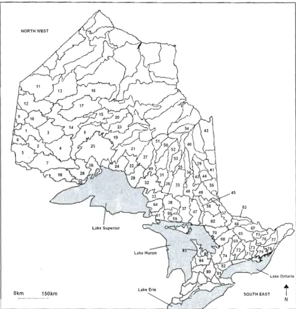
Mikkelson, 2002; Leibold et al., 2004), the Ontario Fish Distribution Database (OFDD), a database, maintained by the Ontario Ministry of Natural Resources (OMNR) containing the presence-absence of 134 temperate lake-fish species distributed among approximately 9900 lakes was used. Species that are introduced, rare (present in less than 0.5% of the lakes) and hybrids, and lakes without species or geographic coordinates were removed, resulting in 53 extant native species and 8911 lakes divided in 85 tertiary watersheds (considered as metacommunities; see Figure 1.1). The average lake richness was 6.46 ± 3.86 fish species. For more information, see the methodology section of Chapter 1. The mean of each environmental variable for the 85 watersheds are presented in Table 1.1. Abbreviations used in Table 1.1 stands for the following: SA
= surface area; P
= shoreline perimeter; ISL
= island
shoreline perimeter; MaxD= max depth; MeanD
=
mean depth; ELEV=
elevation; GDD = growing degree days; SD =secchi depth; TDS=
total dissolved solids; MEl=
morphoedaphic index; Crown=
crown canopy cover; MADT=
mean annual daily temperature; MJT= mean July temperature; MAT
= mean August temperature; and PET = potential evapotranspiration. ISL refers to the size of the combined shoreline perimeter of ail islands present in each lake, hence lakes with no islands will have 13L value of O. MEl is calculated by dividing the total dissolved solids (TDS) present4
in a lake by its mean depth (MeanD). Growing degree-days (GDD) were estimated as follow:
I[((MeanMonthlyTemperature >
S.soC) -S.5°C)
x30]
Where the "30" represent the 30-year recording period of the dataset (Mandrak, 1995). Crown is measured as % of the lake shoreline covered by the canopy of trees (for additiona1 information see Goodchilde & Gale, 1982; Mandrak & Crossman,
1992a).
1.3 -: Community ecology and the metacommunity paradigm
In the last century, many approaches were proposed in order to explain the patterns of species distributions and the processes that regulate them. The classic view is that communities assemble according to niche-related processes, such as resource use and competition. This perspective became very popular among ecologists after Hutchinson's (1957) seminal paper unveiling the multidimensional niche (MacArthur & Levins, 1967; Diamond, 1975). Models based on this approach analyze how niche characteristics su ch as niche breadth (variability in resource use) and marginality (levels of specialization) are affected by the environment and/or biotic interactions (e.g., Mason et al., 2008; Ingram & Shurin, 2009). A few years later, MacArthur & Wilson (1967) proposed the eguilibrium theory of island biogeography (IBT), which states that species composition in insular habitats is dictâted by differences in the area and isolation of sites, which in turn influence the probabi1ity of extinction and colonization of species, respectively (Brown & Kodric Brown, 1977). Ricklefs (1987) reinforced the importance of this approach, but argued that local diversity was not solely dictated by local environment and competition, as it was also largely dependent on the regional pool of potential colonizers and their evolutionary histories. More recently, Hubbell (2001) developed the Unified Neutral Theory of biodiversity which posits that species differences are not relevant (0
community assembly and local community composition \s dictated mainly by stochastic processes such as dispersal, ecological drift and speciation. Although this model has weil fitted some natural systems, space and stochasticity alone cannot explain aIl the variation in species distribution. Thus recently, the metacommunity theory was developed, including both deterministic (i.e., niche).and spatial processes within the same framework (Leibold et al., 2004).
A metacommunity is a set of local communities that are potentially linked by species dispersal at the regional scale (Leibold et al., 2004), whereas a community is the collection of individuals of ail species that potentially interact within a single patch (Holyoak et al., 2005). In this perspective, the spatial distribution of communities and dispersal plays a critical role structuring the species diversity at regional and local scales, which may influence community assembly from what would be expected if only local biotic and abiotic aspects are analyzed (Leibold et al., 2004).
Metacommunities are studied by means of two venues: mechanism (Holyoak
et al., 2005; Driscoll & Lindenmayer, 2009) and structure (Leibold & Mikkelson, 2002; Haudsorf& Hennig, 2007). The mechanistic approach seeks to explain species distribution through several spatially mediated models (e.g., species sorting, patch dynamics, mass-effects and neutral) that have different assumptions about the roles of environment, dispersal rates and stochastic vs. deterministic processes (see Leibold et
al., 2004 for a complete review). The structural approach, which is the focus of this work, evaluates species distributions along environmental gradients that result from specifie mechanisms and manifest as particular patterns of metacommunity structure (Leibold & Mikkelson, 2002; Haudsorf & Hennig, 2007; Presley et al., 2009). In this approach, metacommunity structure is determined by fitting different non-random patterns to an incidence matrix (i.e., site-by-species matrix). Several non-random patterns have been described (see Leibold & Mikkelson, 2002), with sorne being quite common in nature, such as nested subsets (Patterson & Atmar, 1986). Studies
6
addressing patterns of species distributions (e.g., nestedness, Clementsian gradients, Gleasonian gradients, evenly-spaced gradients, checkerboards and random) can provide valuable clues about the factors that regulate ecological communities (Presley et al., 2009), because the mechanisms and theory are unique to each pattern (Presley & Willig, 2010).
Recently, several analytical tools have been developed allowing researchers to identify and accountfor numerous aspects of metacommunity structure (e.g., Hoagland & Collins, 1997; Leibold & Mikkelson, 2002; Haudsorf & Hennig, 2007). In this study, 1 will use the framework developed by Leibold & Mikkelson (2002), termed Elements of Metacommunity Structure (EMS), which is described below.
1.4 - Elements of Metacommunity Structure (EMS)
The EMS technique focuses on determining which pattern best fits to the species distributions within a metacommunity. Prior to analysis, the incidence matrix (i.e., species by sites matrix) is ordered according to the primary axis extracted via correspondence analysis (Presley et al., 2009), which is a common ordination procedure (Gauch et al., 1977) to detect variation in species distributions that respond to latent pro cesses such as environmental gradients (i.e., variation in unmeasured environmental variables). Correspondence analysis (CA) maximizes the proximity of sites with similar species compositions as weil as species with similar distributions (Leibold & Mikkelson, 2002). Therefore, it makes a compromise between minimizing interruptions within species ranges and within community compositions. This reorganization of the data matrix creates a gradient that retlect the integration of
multiple factors (abiotic and biotic) that may be impol1ant in dictating species distributions (Presley & Willig, 2010).
lake environmental variables for each watershed. Abbreviations as outlined on page 4. Watersheds are map of Figure 1.1 P(km) ISL(km) MaxD(m) MeanD(m) ELEV(m) GDD SD(m) TOS(mg/l) MEl CROWN(%) MADT(OC) MJT(·C) MAT(·C) PET(mmlyr) 26.12 2.58 25.94 9.48 361.89 1501.93 3.70 40.41 7.12 98.49 1.80 19.10 17.47 518.27 21.69 4.59 22.20 8.27 388.70 1493.41 3.70 37.38 8.72 93.57 1.91 18.98 17.15 530.60 37.71 1.66 13.52 5.00 387.77 1410.69 2.46 43.37 11.56 99.46 0.98 18.38 16.52 509.13 26.07 4-34 16.06 5.22 41782 1388.00 2.94 38.72 10.82 93.37 1.01 18.14 16.23 508.60 24.79 7.24 26.29 8.49 366.68 1504.57 4.33 36.82 596 9415 2.30 19.23 17.50 538.21 19.41 3.09 21.32 7.65 359.32 1541.11 3.86 33.16 6.98 85.78 2.07 19.35 17.57 538.21 22.01 3.90 23.06 7.64 408.44 1443.86 3.63 29.38 6.07 95.89 1.88 18.46 16.75 525.71 55.58 19.72 19.89 4.77 411.53 1249.73 2.82 24.65 6.97 96.14 -0.22 16.82 14.93 474.57 38.28 31.90 27.66 9.20 356.26 1502.02 3.72 23.49 3.21 99.70 1.23 18.77 17.24 514.91 33.05 6.01 15.68 5.52 392.68 1443.05 2.63 35.07 10.03 93.10 1.05 18.55 16.94 510.18 93.17 22.58 19.53 5.19 31603 1190.93 2.19 40.50 16.28 9633 -0.64 17.64 16.08 502.18 71.58 22.31 18.70 5.74 355.89 1366.44 2.85 27.75 7.21 99.47 0.32 18.20 16.59 513.87 51.78 11.44 12.13 304 330.95 1128.24 2.32 53.29 22.81 99.76 -1.16 17.18 15.45 483.33 86.97 3532 19.02 4.45 402.33 1288.09 3.08 31.93 9.73 98.37 0.01 17.64 15.69 50263 41.61 7.46 13.75 4.08 320.35 1245.58 3.53 78.68 27.56 99.45 -1.28 16.68 14.72 477.08 79.29 16.28 11.08 2.64 298.31 1124.00 230 58.03 29.89 99.97 -1.48 17.00 15.11 473.35 36.93 5.21 10.14 2.63 349.69 1214.00 2.42 62.51 32.72 99.57 -0.67 17.43 15.46 495.35 25.80 4.67 2506 11.65 425.75 142382 3.64 24.25 4.61 :l5.53 1.80 17.39 lG.09 51433 32.17 gO 13.43 3.07 303.88 125138 2.87 88.44 44.93 93.94 -0.54 16.43 14.61 46845 4134 7.70 17.14 4.40 29763 1251.53 3.02 70.41 22.01 99.94 -1.14 16.56 14.70 463.44 18.49 136 16.97 4.53 327.92 1271.34 2.94 97.82 36.79 98.72 0.18 16.15 14.75 481.15 9.45 0.90 15.75 4.47 327.82 1259.68 3.49 86.80 31.03 98.96 082 16.19 14.96 479.69 22.28 4.53 600 1.59 273.86 1261.14 2.39 55.05 3852 1.00.00 -0.91 16.69 14.71 462.23 11.57 0.84 34.50 10.70 340.18 1313.98 4.37 53.63 7.89 97.92 0.94 14.88 14.65 472.09 2233 4.95 24.35 6.61 364.51 1257.10 3.26 56.99 13.86 95.61 0.17 16.33 14.84 479.22 11.04 0.68 18.46 6.10 348.30 1371.86 3.35 75.96 22.98 83.18 1.23 16.50 15.43 501.00 7.58 0.47 14.92 4.54 308.15 1234.58 4.05 112.80 33.22 62.93 0.31 16.62 14.80 481.18
Table 1.1 (continuation) Watershed SA(hec) P(km) ISL(km) MaxD(m) MeanD(m) ELEV(m) GDD SD(m) TDS(mg/l) MEl CROWN(%) MADT("C) MJT(OC) MA Wc) PET(mm/yr) 28 481.52 15.78 4.43 15.63 5.22 445.91 1419.79 2.77 44.71 1627 81.45 1.35 16.88 15.54 502'.69 29 188.28 9.15 0.70 15.44 4.63 373.09 124806 3.53 74.07 23.61 98.77 0.80 15.81 14.61 47658 30 280.08 7.47 0.54 15.33 6.01 456.13 1480.05 3.32 45.55 12.37 84.85 182 17.16 15.86 506.12 31 570.08 26.29 3.33 18.11 5.20 374.08 1316.63 3.10 45.88 13.97 96.04 1.00 16.16 14.87 483.51 32 260.48 14.25 2.07 22.69 6.65 374.60 1316.14 3.97 49.91 13.05 66.88 1.40 15.87 15.11 474.01 33 111.21 8.46 0.94 22.35 6.80 382.81 1378.13 4.89 39.03 8.55 80.83 2.42 16.73 15.99 509.37 34 81.39 6.58 0.51 8.86 2.41 303.49 1353.33 ' 2.56 63.54 44.48 92.84 1.18 17.39 15.70 494.41 35 218.25 11.68 1.94 12.43 3.78 375.48 1371.99 3.53 64.73 27.78 97.45 1.73 17.34 15.79 500.62 36 223.09 12.32 1.76 17.20 4.97 417.67 1362.78 4.12 69.42 19.78 80.87 1.69 16.69 15.50 499.58 37 205.35 13.3 2.6 17.3 6.2 384.9 1545.0 4.4 28.7 6.4 88.4 3.3 18.2 16.6 526.39 38 273.33 17.23 2.64 20.80 6.30 445.40 1448.08 4.22 3361 7.41 98.49 2.75 17.47 16.08 517.84 39 47.44 3.71 0.07 13.14 3.63 287.83 1303.10 2.95 79.67 34.58 9128 0.49 16.76 15.12 485.47 40 200.75 8.00 0.46 16.35 4.41 270.23 1273.27 2.61 82.39 23.85 95.76 0.02 16.46 14.87 482.28 41 1586.30 10.05 5.43 13.09 4.55 297.17 1356.06 3.30 47.29 14.31 97.48 0.74 16.95 15.25 487.08 42 118.13 4.08 0.41 15.54 4.29 296.31 1372.22 3.70 77.75 26.50 80.10 1.09 17.34 1568 49525 43 1054.02 20.92 1.32 5.52 1.78 276.72 1271.80 1.52 36.32 34.40 100.00 -0.50 1582 14.40 471.73 44 68.06 3.64 0.26 11.40 3.93 321.18 1429.67 3.98 68.43 24.85 88.75 1.34 17.56 15.87 506.17 45 94.78 7.48 0.75 20.61 6.39 386.08 1506.80 5.06 58.90 12.34 90.47 2.60 18.44 16.52 524.96 46 140.08 10.01 1.33 14.52 4.37 358.16 1440.08 3.68 56.71 23.82 95.36 1.78 17.90 16.14 511.87 47 149.32 11.97 0.82 18.81 6.71 312.27 1576.62 4.90 37.36 8.09 81.78 3.70 18.79 17.14 528.13 48 142.41 9.40 1.11 15.59 4.96 349.75 1494.38 4.30 44.52 12.95 89.71 2.26 18.25 16.54 524.46 49 736.93 17.38 4.60 12.69 4.25 288.76 1253.97 3.18 108.03 29.55 56.69 0.29 16.52 14.87 474.65 50 256.53 10.24 0.20 8.66 2.86 245.06 1269.03 2.07 70.09 37.08 67.66 0.17 16.68 14.96 473.18 51 34.22 2.74 0.04 13.44 3.93 179.26 1273.62 3.44 111.65 33.81 40.88 0.14 16.96 15.17 473.61 52 178.62 7.15 0.60 9.25 3.06 239.70 1297.43 2.76 99.43 39.05 98.11 0.27 16.81 15.26 475.94 53 83.32 3.73 0.10 10.54 3.40 226.86 1309.89 2.78 98.06 35.35 77.62 0.39 16.94 15.36 479.31 54 21.91 2.37 020 11.07 3.54 224.62 1293.52 3.13 107.19 47.69 85.71 0.10 16.80 15.25 485.33 55 89.46 4.31 0.06 9.70 3.77 258.48 1328.86 2.49 84.66 32.16 48.62 0.77 16.95 15.34 481.79 56 132.43 6.56 0.77 10.88 3.99 308.23 1484.56 283 51.09 20.79 59.30 1.52 17.58 15.95 510.75 co
P(km) ISL(km) MaxO(m) MeanO(m) ELEV(m) GOO SO(m) mS(mg/l) MEl CROWN(%) MAOT("C) MJT("C) MAT(°C) PET(mm/yr) 9.14 0.73 1983 6.19 324.61 1593.29 4.21 4502 1251 87.92 3.45 18.44 17.00 532.03 14.49 2.74 21.53 6.57 308.37 1599.33 4.83 38.47 8.64 90.88 3.13 18.54 16.93 527.42 9.59 0.67 24.06 8.55 312.43 163628 5.32 39.86 8.15 87.37 431 18.60 17.27 530.19 6.41 0.23 22.80 8.02 387.75 1512.92 5.59 30.08 7.13 89.66 3.56 1812 16.65 527.48 7.10 0.65 17.74 6.70 325.94 1514.57 4.07 29.43 7.40 65.77 3.65 17.44 16.60 524.00 11.41 1.30 16.27 5.12 277.09 1708.07 3.00 28.96 8.60 60.80 4.42 18.92 17.53 537.63 331 0.07 10.53 3.60 237.23 1745.64 2.71 2833 11.43 82.08 3.85 18.70 17.33 542.03 5.91 0.56 16.66 5.21 400.23 145487 4.24 2553 7.82 81.41 3.01 16.83 16.07 512.72 5.61 0.44 15.72 5.18 397.95 1704.14 3.89 56.07 16.36 74.05 4.07 18.38 16.95 542.73 11.41 1.32 19.32 6.31 348.93 1678.99 3.99 29.07 7.30 96.07 3.74 18.22 16.81 542.73 5.08 0.23 14.07 4.71 242.48 1828.00 3.66 65.44 20.34 50.79 4.40 18.99 17.59 546.35 8.60 1.54 16.32 5.75 346.58 168904 3.86 24.24 6.81 52.42 4.65 18.74 17.47 542.73 7.33 0.61 22.26 7.82 36557 1714.45 4.99 42.41 9.00 26.93 4.47 1855 17.26 543.45 8.94 1.11 14.20 5.02 297.54 1723.79 357 25.37 758 53.67 ·4.67 18.85 17.56 542.01 7.12 0.96 14.11 4.75 325.26 1805.65 389 93.80 31.79 38.73 5.07 18.99 17.78 545.13 12.14 2.11 15.03 4.76 306.25 1819.75 3.47 64.22 30.46 65.58 5.36 19.24 18.13 540.63 8.0 1.1 12.7 4.9 244.0 1886.2 2.7 104.6 355 46.9 5.4 19.4 18.3 548.83 6.53 0.80 1118 4.06 277.44 1808.81 2.99 61.74 42.00 52.71 5.38 19.31 18.15 550.88 4.99 0.23 14.52 5.24 289.92 1867.06 4.17 11440 43.17 73.35 4.77 19.40 18.01 543.54 737 0.97 13.11 4.45 247.58 1930.55 3.71 10Z.I:l:;l fi4.25 3535 5.11 19.60 1825 543.7b 17.43 1.10 16.73 5.69 14810 1999.46 3.50 133.04 115.41 2.86 5.94 20.32 19.00 557.92 14.19 2.96 19.79 7.28 13011 1999.69 3.57 114.81 38.45 21.82 6.07 2029 19.03 563.02 9.0 05 17.6 5.7 174.0 1990.4 3.6 108.1 45.6 33.7 5.8 19.8 18.6 550.89 2.56 0.37 4.76 195 328.00 2188.58 1.69 227.42 185.75 5.69 6.92 20.21 19.16 571.91 1.74 0.05 5.35 1.91 34735 2119.91 2.35 237.26 223.76 0.00 6.61 19.93 18.93 565.68 1.47 0.04 8.87 2.68 256.17 2207.61 1.72 242.43 186.03 8.26 7.09 20.54 19.50 580.69 4.35 0.36 3.38 1.15 207.06 1782.63 2.05 19554 331.69 11.84 5.87 19.05 18.12 546.06 1.70 0.06 5.50 220 340.03 1889.49 2.64 253.97 195.57 5.31 5.95 19.04 18.01 556.50 3.64 0.30 4.77 1.92 353.22 1891.57 2.35 233.74 202.67 15.22 5.88 18.96 18.10 551.28
10
EMS is based on three fundamental elements (see Figure 1.2) of the binary incidence matrix, after reordered through correspondence analysis: coherence, species turnover and boundary clumping (Leibold & Mikkelson, 2002). Coherence is calculated by counting the number of embedded absences (i.e., absences between presences) within species ranges or community compositions. Turnover is evaluated by counting the number of times two sites exchange two species. Finally, boundary clumping is the assessed by the Morisita index (Morisita, 1971), representing the degree of coincident range or community boundaries in the matrix (Leibold & Mikkelson, 2002). The significance of each element is assessed by a nul! model analysis, which is described in the methodology section of Chapter one. Using the interaction between these three basic elements of the incidence matrix, six different patterns can be distinguished: checkerboards, Clementsian gradients, Gleasonian gradients, evenly-spaced gradients, nested subsets and random distributions (See Figure 1.2).
Checkerboard patterning fol1ows from Diamond (1975) fifth assembly rule which states that "some pairs of species never co-occur, either by themselves or in larger combinations, mainly due to competition" (Diamond, 1975). In this case the incidence matrix has significantly negative coherence (i.e., more embedded- absences than expected by chance), which means that the metacommunity is composed by pairs of mutually exclusive species that occurs independently of one another (Presley
et al., 2009).
Clementsian and Gleasonian gradients come from an historical debate JO community ecology that mainly focused on vegetation commuilities (Hoagland & Collins, 1997). One side argued that biotic communities are a discrete group of species that show similar responses to environmental factors (Clements, 1916) and
Figure 1.1 Map of Ontario divided by tertiary watersheds (Cox, 1978), with
corresponding codes from Table 1.1. Watersheds without codes have no data available. Map adapted from Ministry of Environment (2004).
12
replace each other across space (Hoagland & Collins, 1997), whereas the other suggested that species have somewhat individual responses to abiotic factors and communities form a continuum of gradually changing compositions along the environmental gradient (Gleason, 1926). These ideas were recently extended to deal with animal communities as weil (Leibold & Mikkelson, 2002, Heino, 2005; Presley
et al., 2009). Evenly-spaced gradients occur in metacommunities where species are
competing along an environmental gradient and species distribution is dictated by trade-offs in their ability to explore alternative resources (Tilman, 1982; Leibold & Mikkelson, 2002). Ali three patterns appear in coherent metacommunities that exhibit positive turnover. The difference is in boundary c1umping, where boundaries can be either clumped in Clementsian gradients, randomly distributed in the Gleasonian gradients or hyperdispersed in evenly-space gradients (Leibold & Mikkelson, 2002).
Nested subsets arise in sets of sites where poor-species biota are predictable subsets of the species composition from richer biota, i.e~, common species- occur at most sites and rare species occur only in the most diverse communities (Patterson & Atmar, 1986). Biotic nestednesshas been found to be structuring the distribution of a large number of taxa (Wright et al., 1998) and appears to be a common pattern in fragmented landscapes such as islands, isolated mountain tops and fragmented forest patches (Cook & Quinn, 1995; Patterson & Atmar, 1986; Honnay et al., 1999;
Férnandez-Juridic, 2002). Many studies have found that the main ecological processes driving nested patterns are selective colonization and selective extinction (e.g., Cook & Quinn, 1995; McDonald & Brown, 1992) which are related to differences in patches isolation and area, respectively. However, other causes for nested distributions have been also proposed, such as passive sampling, nested habitats, selective environmental tolerances and environmental harshness (see Ulrich
et al., 2009 for a complete review). In this case, the metacommunity is coherent and
exhibits low turnover rates among communities due to sorne degree of overlap between their species composition. Finally, a metacommunity can exhibit non
significant coherence, which suggests that species are not responding to the same environmental gradient and are c1assified as random (Presley et al., 2009).
Although these patterns are weil studied in the ecological literature (e.g., Hoagland & Collins, 1997; Leibold & Mikkelson, 2002; Haudsorf & Hennig, 2007; Presley et al., 2009; Ulrich et al., 2009), there has been no attempt to compare different patterns across several metacommunities within the same system (but see Presley & Willig, 2010). Part of the problem is that large data sets which encompass several metacommunity systems over an entire biogeographic region are rare. This issue will be overcome by using the OFDD, because of the large number of lakes (n=8911) and the possibility to divide the set among somewhat discrete metacommunity units (e.g., watersheds), allowing comparisons among EMS patterns. Because each pattern can be considered a different "metacommunity trait", that are patterned by different structuril1g mechanisms, comparisons among patterns can increase our knowledge about how biological communities are structured over space, history and environmental gradients (Leibold & Mikkelson, 2002).
1.5 - The phylogenetic structure of ecological communities
Another important issue to consider in metacommunity studies is the evolutionary history of species (Loeuille & Leibold, 2008). In the last decade, the phylogenetic aspects of community assembly have gained increasing attention from ecologists (Webb et al., 2002; Cavender-Bares et al., 2009; Peres-Neto, 2004; Kraft
et al., 2007). Because species that diverged recently (i.e., species close within a
phylogenetic tree) tend to be ecoLogically similar (Cavender-Bares et al., 2004; Peres Neto, 2006), there may be a link between the phylogenetic relatedness of taxa and the factors that determine their distributions (Leibold et al., 2010). Assuming that species niches are somewhat conserved through time (i.e., closely related species diverge less through time than of what would be expected in an unconstrained evolutionary
14
@
___
~ ~I:I CheCkerboardS)•
'---v-J L _ _~III--,-R;.=a"","nd::.;;o,,,m,--...,)~1c
L
__
~I:I.
Nestedness )•
• Evenly-Spaced-)1
Il
Gleasonian ) • P,Ot:'1I"r.. :.j AM.t!.:.Figure 1.2 General framework for the Elements of Metacommunity Structure (coherence, turnover and boundary clumping). Columns represent sites and rows represent species. NS = non significant. See Table 1.2 for EMS results of the
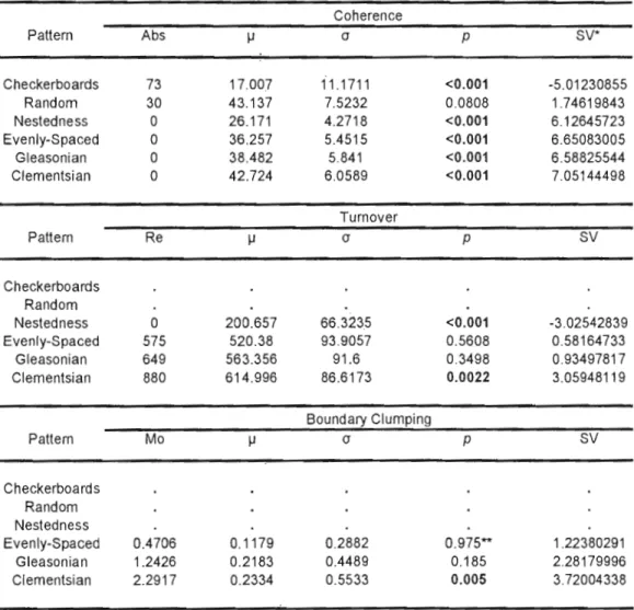
Table 1.2 Results of EMS analyses on hypothetical matrices from Figure 1.2. Analyses were performed using the first ordination axis extracted via reciprocal averaging and based on community perspective. Abs = number of embedded absences; Re
=
number of replacements; Mo= Morisita's index;
!..l.= mean value of
each element for the random distribution; (J = standard deviationof each element for the random distribution; p=
significance probability; SV= standardized value.
Significant results (p:s
0.05) are in boldo *Coherence standardized values were multiplied by -1 ** Mo is statistically tested with a two-tailed test, thus when p 2:0.95, the result is significant and indicate an evenly-spaced gradient metacommunity pattern. Coherence Pattern Abs cr p sv* Checkerboards Random Nestedness Evenly-Spaced Gleasonian Clementsian 73 30
o
o
o
o
17.007 43.137 26.171 36.257 38.482 42.724 11.1711 7.5232 4.2718 5.4515 5.841 6.0589 <0.001 0.0808 <0.001 <0.001 <0.001 <0.001 -5.01230855 1.74619843 6.12645723 6.65083005 6.58825544 7.05144498 Pattern Re Turnover cr p sv Checkerboards Random Nestedness Evenly-Spaced Gleasonian Clementsiano
575 649 880 200.657 520.38 563.356 614.996 663235 93.9057 91.6 86.6173 <0.001 0.5608 0.3498 0.0022 -3.02542839 0.58164733 0.93497817 3.05948119 Pattern Mo Boundary Clumping cr p sv Checkerboards Random Nestedness Evenly-Spaced Gleasonian Clementsian 0.4706 1.2426 2.2917 0.1179 0.2183 0.2334 0.2882 0.4489 0.5533 0.975*" 0.185 0.005 1.22380291 2.28179996 3.7200433816
process; Wiens & Graham, 2005), phylogeny can assist in disentangling two main opposing processes of community assembly: habitat filtering, where communities are composed of species that share similar environmental tolerances (Webb, 2000), and competitive-exclusion, where species that are ecologically similar cannot co-exist in the same local communities due to high overlap in resource use (MacArthur & Levins, 1967; Mason et al., 2008). If the first process is dominating, co-occurring species are expected to exhibit a pattern of phylogenetïc clustering (Cavender-Bares et al., 2006); however, if the second process is the most important, communities will be composed of distant-related species (i.e., phylogenetic overdispersion) due to competitive exclusion of species that use similar resources. If niche is not conserved through time due to, for instance, convergent evolution due to natural selection, phylogenetic results have less power to detect non-random community assembly processes (Losos, 2008).
Both processes (e.g., habitat filtering and limiting similarity) can influence patterns and dynamics observed at the metacommunity level (PillaI' & Duarte, 2010). For example, Clementsian gradient is a pattern that occurs in metacommunities where clusters of communities are formed by a discrete group of species that can either show a similar response to environmental gradients (Presley et al., 2009) or be a result of "clumped competitive exclusion" (Gilpin & Diamond, 1982). Evidence for these mechanisms can be obtained by a community phylogenetic analysis: if co occurring species are closely related and present phylogenetic niche conservatism than it might suggest that environmental filtering is selecting species with similar tolerances to the environment (Cavender-Bares et al., 2009) and structuring the Clementsian gradient pattern at the metacommunity level. However, if co-occurring species are more distantly related in the phylogeny, than two processes can be suggested: 1) competitive interactions are precluding long-term co-existence between species that present phylogenetic niche conservatism and thus similar ecologicaJ characters (Cavender-Bares et al., 2004); 2) Phylogenetic distant related species
present similar ecological characteristics due to convergent evolution resulting [rom environmental filtering (Losos, 2008). Thus, after finding the pattern that best fit the species distributions within a metacommunity, we can use the phylogenetic approach to seek for possible structure mechanisms that dictate these patterns.
A COMMUNITY OF METACOMMUNITIES: EXPLORlNG PATTERNS fN
SPECIES DISTRIBUTIONS ACROSS LARGE GEOGRAPHICAL AREAS
Une communauté de metacommunautés: Exploration des patrons de distribution d'espèces à travers de larges aires géographiques
20
2.1 - Introduction
2.1.1 - Metacommunities: Structural versus Mechanistic approach
Unraveling and disentangling multiple mechanisms influencing the composition and variation of ecological communities across space is a central problem and intellectual challenge in biology (Ricklefs, 1987; Gaston, 2000; Holyoak et al., 2005). Research based on spatial patterns of biodiversity seeks to identify the set of abiotic and biotic process (and how they interact) that define how subsets of species (i.e., local communities) are filtered down from those found in the larger regional species pool of potential colonizers (Gotelli and Graves, 1996; Jackson et al., 2001; see also Figure 3.2 in chapter two).
There is a growing consensus among ecologists that both large-scale processes and local factors need to be considered in order to understand spatial patterns of biodiversity (Ricklefs, 2004; Holyoak et al., 2005). In this context, metacommunity is the fastest advancing framework in spatial ecoJogy because it accounts for both local (e.g., environment) and regional (e.g., dispersal) processes (Leibold et al., 2004). In this framework, a metacommunity is defined as a set of local communities that are potentially linked, but not necessarily, by dispersal of individuals of species across local communities (Leibold et al., 2004; Holyoak et al., 2005).
Metacommunities have been mainly studied by two approaches: the mechanistic approach (Holyoak et al., 2005; Muneepeeraku et al., 2008; Driscoll & Lindenmayer, 2009), in which the focus is on determining the predominance (or their relative importance, e.g., Cottenie 2005) of distinct model processes (e.g., species sorting, patch dynamics, mass-effects and neutral) regarding different assumptions underlying metacommunity dynamics. Sorne of these assumptions involve species trade-offs, dispersal rate differences across species and communities, the presence of environmental gradients and stochastic versus deterministic processes (Leibold et al., 2004); and 2) the structural approach (Leibold & Mikkelson, 2002; Heino, 2005;
Hausdorf & Henning, 2007; Presley et al., 2009; Presley & Willig, 2010), which focuses on understanding non-random patterns in the structure of the distributions of species across communities represented by species incidence or abundance matrices. Uncovering large-scale distributional patterns is an essential source of inferences about the causes driving variation in species composition across communities (Gotelli and Graves 1996; Peres-Neto, 2004; Werner et al., 2007). Identifying the forces structuring these patterns can provide clues about the underlying processes driving species co-occurrence and site occupancy mechanisms. In this work, l will focus on the latter approach given that under only certain conditions we can estimate the likelihood of the different models under the mechanistic approach (Legendre et al., 2008; but see Cottenie, 2005).
The analysis of patterns in incidence matrices in order to determine the degree of negative and positive associations across species has a long history of applications in ecology (Diamond, 1975; Connor & Simberloff, 1979; see Gotelli & Graves, 1996 for a review). Although this species-guided approach has provided important insights into ecological processes structuring ecological communities, it has been somewhat limiting because it does not take into account the organization of sites that may also influence species co-occurrences patterns. For instance,. species along environmental gradients may be organized into blocks of species overlapping in their distribution. Species within blocks may appear positively associated due to common habitat affinities, whereas species across blocks may appear negatively associated due to differences in habitat across environmental gradients. Indeed, more recently, ecologists have been exploring a dual species and community (site) perspective (Leibold & Mikkelson, 2002). Perhaps the most weil known of these incidence patterns is the nested species subsets in which commul1ities of successively fewer species contains subsets of those species found on the next richer community (Patterson & Atmar, 1986).
22
Leibold & Mikkelson (2002) developed a framework termed Elements of Metacommunity Structure (EMS) that analyzes several possible patterns that take into account this dual arrangement of communities and species. In their EMS framework, the interaction between three different elements (i.e., coherence, turnover and boundary c!umping) generates six different possible patterns of species distribution across communities, which have been referred as to nestedness, Clementsian gradients, G1easonian gradients, evenly-spaced gradients, checkerboards and random (Figure 1.2). In this approach, each pattern assumes that species distributions are a result of particulaI' species responses to abiotic and biotic factors along a major distributional gradient of species across sites (Leibold & Mikkelson, 2002; although multiple interacting gradients could provide greater refinement, little analytical progress has been made in this direction; but see Presley et al., 2009). The interactions of each metacommunity element described above (i.e., coherence, turnover and boundary c1umping) make predictions about the six above mentioned metacommunity patterns. When species do not respond to the same environmental gradient (i.e., different habitat affinities), the metacommunity (i.e., distribution of species across communities embedded in local sites) will present a random structure (Presley & Willig, 2010). If metacommunities are composed of pairs of mutually exclusive species that occur independently of other pairs along the gradient, they are classified as checkerboards (Diamond, 1975). Nestedness occurs on metacommunities with low turnover rates, where the composition of poor-species sites represents proper subsets of progressively richer sites (Ulrich et al., 2009; see above). Wh en turnover rates (i.e., changes of species compositions across communities) are higher than expected, metacommunities can be c1assified as Clementsian, Gleasonian or evenly-spaced gradients. The first one indicates that biotic communities are a discrete group of species that shows simiJar responses to the gradient and replace each other on space across the rnetacommunity (Clements, 1916). Gleasonian gradients represent communities composed of species that show idiosyncratic responses to the gradient, yielding a metacommunity with a form of a
continuum of gradually changing composition (Gleason, 1926). Finally, metacommunities defined as evenly-spaced gradients are composed by species supposedly competing along a gradient and their distribution will be dictated by trade-offs in their abilil)' to explore alternative resources (Tilman, 1982; Leibold & Mikkelson, 2002).
Although a large number of studies have assessed some of these EMS patterns separately (e.g., nestedness, Cook & Quinn, 1995; Wright et al., 1998; Fernandez Juricic, 2002; Leprieur et al., 2009; checkerboards, Diamond, 1975; Connor & Simberloff, 1979; Gilpin & Diamond, 1982), to date only a few studies haveapplied this approach to test which pattern best fltS to a given metacommunity data (studies were reviewed by Presley et al., 2009), or compared patterns within metacommunities across different systems (e.g., Leibold & Mikkelson, 2002).
2.1.3 - Looking further into EMS framework
The EMS approach is extremely promising because it allows characterizing metacommunity patterns across different taxa, metacommunities and ecosystems, providing an exceptional venue to search for general rules in determining .. the structure of community assemblages across space. For instance, two bird and two plant metacommunities, each taxa combination (i.e., one bird and one plant) being in different climatic zones (tropical versus temperate) may show different EMS patterns across taxa (i.e., bird versus plant) but similar within regions (e.g., nested plant and bird in tropical region and Gleasonian gradients plant and bird in the temperate region). In this case, the conclusion would be that the climatic zone is driving the pattern. Although promising, this comparative approach either across taxa or region has yet to be explored. To my knowledge, only one study has looked at how these elements of metacommunities compare across different regions for the same taxa (i.e., bat metacommunity structure on Caribbean islands; Presley & Willing, 2010). However, their study was also limited by the fact that they only have three regions
24
and therefore little inference can be made about how differences between regions could have explained the observed patterns.
Given that each EMS pattern can be considered as a different "metacommunity trait" with unique underlying structuring mechanisms and theory (Leibold & Mikkelson, 2002; Hoagland & Collins, 1997), exploring and comparing such patterns across large geographical regions has the potential to enhance our understanding of how biological communities respond to environmental (Presley et
al., 2009) and biogeographical variation. Moreover, insights on key ecologica1
patterns such as ~-diversity (Leprieur et al., 2009) might be acquired throughout such comparisons (e.g., nestedriess versus turnover; Hausdorf & Hennig, 2007).
2.1.4 - Lake-fish systems as metacommunities
Lakes within a watershed can be considered as "viltual islands" (Magnuson et
al., 1998) varying in size, environmental features (Eadie et al., 1986) and degree of
isolation (Olden et al., 2001), which may impose different environmental and spatial constraints which in turn will influence fish dispersal and probability of establishing viable populations, as weil as their extinction vulnerability (Magnuson et al., 1998;
Olden et al., 2001). Indeed, some studies have found that local environment was the most important predictor of lake-fish species distribution (e.g., Magnuson et al.,
1998) whereas others have found that spatial (i.e., regional) factors were the most prevalent (e.g., Beisner et al., 2006). This dichotomy shows that different lake-fish metacommunities can be structured by different factors, but little is known whether there are general assembly patterns emerging from these processes. The search for general rules that may dictate patterns that best reflect the distribution of species within a metacommunity should increase our understanding about the underlying mechanism structuring metacommunities (Leibold & Mikkelson, 2002; Heino, 2005). To date no study has investigated whether and how local and regional features generate consistent patterns across different metacommunities.
2.1.5 - Chapter objectives
1 used a unique data set containing environmental and presence-absence data on fish distribution on about 9000 boreal lakes from Ontario, Canada, across 85 metacommunities (watersheds). The approach used here was the following: 1) classify each fish metacommunity (i.e., watershed) according to EMS patterns; 2) determine the relative influence of spatial and environmental factors within and across metacommunity EMS patterns.
2.2 -Methodology
2.2.1 - Ontario Fish Distribution Database (OFDD)
1 used a lake-fish database, the Ontario Fish Distribution Database (OFDD), maintained by the Ontario Ministry of Natural Resources, which contains presence absence records of 134 fish species (including 7 hybrids) and geographic positions for approximately 9900 boreal lakes (inland lakes only) from Ontario. Records span from 1900 to 1992,however most lakes were sampled between 1968 and 1985. The OFDD is known to have sampling biases, where sport fishes are overrepresented and small-bodied species, such as cyprinids, are underrepresented (Minns, 1986). The full history of the dataset can be found in Mandrak and Cross man (1992a) and the sampling methods in Goodchilde and Gale (1982). Despite the potential sample biases and the fact that collection spanned over a long period, this dataset has been providing important insights in many different types of ecological research (Mandrak, 1995; Gonzalez & Gardezi, 2008; Sharma et al., 2009). Finally, given that 1 am interested in broad regional-scale patterns, sampling biases should be diluted across reglüns.
2.2.2 - Lake Inventory Database (LINY)
Information about the local environment in each lake was assessed using the Lake Inventory Database (LINY), a dataset that includes the following environmental
26
variables for each lake in the OFDD: surface area (SA), shoreline perimeter (P), island shoreline perimeter (ISL), mean depth (MeanD), maximum depth (MaxD), secchi depth (SD), growing degree days (GDD), eJevation (El ev), total dissolved solids (TDS), morpho-edaphic index (MEl), mean annual daily temperature (MADT), canopy cover (Crown), mean July temperatures (MJT) and mean August temperatures (MAT). Missing values were replaced by the mean value of that variable within the watershed; 0.2% of the lakes on average per variable were replaced. Note that the environmental information of lakes treated in this way became uninformative, specially compared to the total number of lakes used in the analysis (n ;:::;: 9000). l have also considered values of potential evapotranspiration (PET) which serves as a proxy of thermal energy that is in turn correlated with lake productivity (Gonzalez & Gardezi, 2008). This variable was missing for a large number of lakes, but has low variability within watersheds (see Gonzalez & Gardezi 2008 for details on how this measure was estimated), and therefore was only used in analyses among watersheds In this case, 1 used the mean PET from ail lakes that were available for any given watershed. Finally, lakes with missing geographic coordinates or without species were removed from the analyses.
2.2.3 - Species used in the analyses
Species that were present in less than on an arbitrary value of 0.5 % of ail lakes in the data set were removed. Rare and endemic species are somewhat uninformative due to its idiosyncratic nature, but they can affect EMS analysis in ways that will not be discussed here (but see Presley & Willig, 2010). Introduced species were also removed because they do not follow any historical contingency experienced by the native species. In total, 53 extant native species across ail lakes were used in analyses (Table 3.1; Chapter 2).