Unsteady Numerical Simulations of Transcritical Turbulent Combustion in Liquid Rocket Engines

(1)

Institut National Polytechnique de Toulouse (INP Toulouse)

École doctorale et discipline ou spécialité : ED MEGEP : Énergétique et transferts

Anthony Ruiz

9 Février 2012

Simulations Numériques Instationnaires de la combustion turbulente et

transcritique dans les moteurs cryotechniques

(Unsteady Numerical Simulations of Transcritical Turbulent Combustion

in Liquid Rocket Engines)

CERFACS

B. Cuenot - Chef de projet CERFACS, HDR L. Selle - Chargé de recherche CNRS

F. Dupoirieux - Maître de Recherches à l’ONERA, HDR J. Réveillon - Professeur à l'Université de Rouen

S. Candel - Professeur à l'Ecole Centrale Paris P. Chassaing - Professeur émérite à l'INPT

D. Saucereau - Ingénieur SNECMA

(2)

(3)

List of Figures

1.1 The main components of the Ariane 5 european space launcher. . . 1 1.2 Components of a booster. . . 2 1.3 Operating principle of the Vulcain 2 engine [Snecma 2011]. . . 3 1.4 Injection plate of the Vulcain 2 LRE, composed of 566 coaxial injectors

[As-trium 2011] . . . 3 1.5 Heat capacity isocontours computed with the Soave-Redlich-Kwong

equa-tion of state (see Eq. 2.44): white = 103 _{J/K/kg; black=10}4 _{J/K/kg. . . .} ₅

1.6 Shadowgraphs at successive instants (time between frames is 0.1 ms) of a transcritical N2/supercritical He mixing layer [Teshome et al. 2011]. . . 8

1.7 Flame shape visualizations using OH∗_{, in a coaxial LOx/GH}

2 injector

[Ju-niper 2001]: (a) instantaneous image, (b) top: time-averaged image; bot-tom: Abel-transformed image. The pressure is 7 MPa. . . 9 1.8 OH PLIF image of a LOx/GH2 cryogenic flame [Singla et al. 2007]. . . 10

1.9 Shadowgraphs of a transcritical H2/O2 reacting flow at 6 MPa, taken at

successive instants (time between frames is 0.25 ms) [Locke et al. 2010]. . . 10 1.10 Schematic of coaxial jet injector and the near-field mixing layers

[Schu-maker & Driscoll 2009] . . . 11 1.11 Radial distributions of normalized density at diﬀerent axial locations (T∞=

300 K, uinj = 15 m/s, Tinj = 120 K, Dinj = 254 µm) [Zong & Yang 2006] . 14

1.12 Contours of temperature for the near-field region for (a) supercritical and (b) transcritical mixing [Oefelein & Yang 1998]. . . 15 1.13 LES computations of transcritical jet flames: (a) T = 1000 K iso-surface

colored by axial velocity in a reacting transcritical LOx/GH2 flow

[Mat-suyama et al. 2010]. (b) Visualization of a transcritical LOx/GCH4 flame:

(top) direct visualization from experiment [Singla 2005]; (bottom) T = (Tmax_{+ T}min_)/2 _{isosurface from LES [Schmitt et al. 2010a]. . . 17}

1.14 Schematic of a LRE combustion chamber, showing the diﬀerent levels of study considered in the present thesis work. . . 18 2.1 Transport coeﬃcients for O2 at 100 bar, showing the liquid-like to gas-like

transition of thermo-physical properties . a) Dynamic viscosity b) Thermal conductivity. . . 23 2.2 Evolution of the Lewis number and normalized heat capacity with

temper-ature. Cp,0 = 1700 J/K/kg. The peak of Cp at the pseudo-boiling point

creates a local minimum in the Lewis number. . . 24 2.3 Density of oxygen as a function of temperature, at 10 MPa, computed

with the Peng-Robinson and the Soave-Redlich-Kwong equations of state, and compared to the NIST database [Lemmon et al. 2009]. The circle at T = 172 K shows the pseudo-boiling point. . . 30

(6)

6 List of Figures

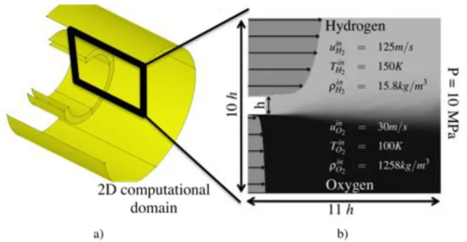
3.1 a) Typical coaxial injector of a LRE. b) Boundary conditions for the 2D computational domain . . . 35 3.2 Probes located in the mixing layer. . . 39 3.3 Transverse cut through the initial solution of the cold flow, downstream

the lip. . . 40 3.4 Temporal evolution of the minimum, mean and maximum pressures in the

computational domain, after instantaneous ignition of the cold flow case. . 41 3.5 Strained diﬀusion flame computed in AVBP: streamlines superimposed on

the temperature field. Thermodynamic conditions correspond to the split-ter case: hydrogen at 150 K from the top, oxygen at 100 K from the bottom and ambient pressure is 10 MPa. . . 42 3.6 Comparison of flame structure versus mixture fraction between AVBP and

CANTERA. (a) temperature and (b) HO2 mass fraction. The vertical bar

indicates the stoichiometric mixture fraction. . . 43 3.7 Major species mass fractions as a function of mixture fraction for the

non-premixed counterflow flame configuration (lines) and equilibrium (symbols) 44 3.8 Non-reacting flow: axial velocity field, showing the shear-induced

Kelvin-Helmholtz instability. . . 45 3.9 Non-reacting flow: oxygen mass fraction field at the H2 corner of the lip,

at successive instants. The time interval between frames is 10 µs . . . 46 3.10 Non-reacting flow: O2 mass fraction field, showing the rapid mixing of the

two streams by a large range of vortical structures. . . 46 3.11 Non-reacting flow: temporal evolution of the transverse velocity field. The

time interval between two snapshots is τconv . . . 48

3.12 Non-reacting flow: temporal evolution of the oxygen mass-fraction field. The time interval between two snapshots is τconv . . . 49

3.13 Non-reacting flow: transverse velocity signal analysis. Top) temporal signal; dominant harmonic (St = 0.14). Bottom) Power Spectrum

Density without spectrum averaging. . . 50 3.14 Non-reacting flow: eﬀect of the Welch averaging procedure on the spectrum

frequency resolution. Number of windows=2,4,8. . . 50 3.15 Non-reacting flow: spatial evolution of the transverse velocity spectrum in

the wake of the lip. Eight Welch averaging windows are used. . . 51 3.16 Non-reacting flow: power spectrum density of the squared transverse

ve-locity at i=10, j=12. Eight Welch averaging windows are used. . . 52 3.17 Non-reacting flow: vorticity field superimposed on the high-density region

(fluid regions with a density that is higher than ρ0.5 = 0.5 (ρinjH2 + ρ

inj O2)are

painted in black.). . . 53 3.18 Non-reacting flow: O2 mass fraction, along with a grey isocontour of

mid-density (ρ = 637 kg.m−3_{) and a white isocontour of high scalar dissipation}

rate (χ = 5 103_s−1_{). The dash circle shows a region of low scalar dissipation}

rate where mixing has already occurred. . . 54 3.19 Non-reacting flow: conditioned average and maximum value of scalar

(7)

List of Figures 7

3.20 Non-reacting flow: average density field . . . 56 3.21 Non-reacting flow: spreading angles θρ,α. . . 57

3.22 Non-reacting flow: transverse cuts of the density at 4 axial positions be-tween x=0h and x=6h. . . 58 3.23 Non-reacting flow: transverse cuts of the RMS axial velocity normalized

by the velocity diﬀerence Us = U_Hinj₂ − U_Oinj₂ at x=1h and x=5h. . . 58

3.24 Non-reacting flow: transverse cuts of the RMS transverse velocity normal-ized by the velocity diﬀerence Us = UHinj2 − U

inj

O2 at x=1h and x=5h. . . 59

3.25 Instantaneous snapshots of the transverse velocity and the density for the (a) h100 and (b) h500 meshes. . . 60 3.26 Mean profiles, at x = 5h for the h100 and h500 meshes of (a) axial velocity,

(b) transverse velocity and (c) O2 mass fraction . . . 61

3.27 RMS profiles, at x = 5h for the h100 and h500 meshes, of (a) axial velocity, (b) transverse velocity and (c) O2 mass fraction. . . 62

3.28 Temperature field with superimposed density gradient (green) and heat-release (black: max heat heat-release rate of case AVBP_RG (=1013 _W/m3_);

grey: 10 % of case AVBP_RG (=1012 _W/m3_{). . . 63}

3.29 Close-up view of the flame stabilization zone behind the splitter. Tempera-ture field with superimposed iso-contours of density gradient (green=4 107_kg/m4₎

and heat-release rate (grey=1012 _W/m3_{, black=10}13 _W/m3_{). . . 64}

3.30 The flame/vortex interaction separates the flame into 2 zones, a near-injector steady diﬀusion flame between O2 and a mixture of H2 and H2O,

and a turbulent flame developing further downstream. . . 65 3.31 Comparison of the density fields between a) the non-reacting flow and b)

the reacting flow . . . 66 3.32 Curvature PDF of the median density (ρ0.5 iso-contour for the cold and

reacting flows. . . 66 3.33 Reacting flow: instantaneous fields of (a) hydrogen (b) oxygen and (c)

water mass fraction, with superimposed stoichiometric mixture fraction isoline (black). The dash line in (b) shows the location of the 1D cut that is used in Fig. 3.34. . . 67 3.34 Cut through a pocket of oxygen diluted with combustion products. The

location of the 1D cut is shown by a dash line in Fig. 3.33(b). . . 69 3.35 Flame structure in the mixture fraction space. counterflow diﬀusion

flame at a = 3800 s−1_{, • scatter plot of the present turbulent flame. . . 70}

3.36 Average density field for the reacting flow. White iso-contour: ρ = 0.9 ρin O2. 71

3.37 Average fields for the reacting flow. (a) Temperature. (b) Heat release rate. Black iso-contour: ρ0.9. . . 72

3.38 OH mass-fraction fields at four instants. Liquid oxygen and gaseous hy-drogen are injected below and above the step, respectively. . . 73 3.39 OH-PLIF images of the flame holding region. Liquid oxygen and gaseous

hydrogen are injected above and below the step, respectively (opposite arrangement of Fig. 3.38). The OH distribution in the flame edge is shown on the standard color scale. p = 6.3 MPa (fig. 5 of [Singla et al. 2007]) . . 74

(8)

8 List of Figures

3.40 Comparison between experimental signal of OH PLIF [Singla et al. 2007] at transcritical conditions and time averaged heat release rate in the current simulation (the numerical visualization is upside down to compare with experimental visualization) . . . 75 4.1 Square combustion chamber with optical access used in the Mascotte facility. 79 4.2 Geometry of the coaxial injectors: a) dimensions and b) recess length. . . . 80 4.3 Cut of the h5 mesh, colored by ∆ = V1/3_{, with V the local volume of cells. 81}

4.4 Species mass fraction as a function of mixture fraction, in the infinitely fast chemistry limit (Burke-Schumann solution). . . 83 4.5 Turbulence injection profiles: a) mean axial velocity and b) Root Mean

Square velocity fluctuations. The superscript c refers to the centerline value. 85 4.6 Instantaneous visualization of the reacting flow: a) temperature and b)

axial velocity fields. . . 87 4.7 Qualitative comparison between instantaneous experimental ((a) and (c))

and numerical ((b) and (d)) visualizations of the reacting flow: (a) OH∗

emission (b) T = 1500 K iso-surface (c) shadowgraph (d) mixture fraction between 0 (black) and 1 (white). . . 89 4.8 Instantaneous a) axial velocity and b) temperature cuts. . . 90 4.9 Qualitative comparison between instantaneous experimental ((a) and (c))

and numerical ((b) and (d)) visualizations of the near-injector region of the reacting flow: (a) OH∗ _{emission (b) T = 1500 K iso-surface (c)}

shadow-graph (d) mixture fraction (black=0; white=1). . . 91 4.10 Cut of the average velocity magnitude (white = 0 m/s; black = 200 m/s)

with superimposed streamlines in black and density iso-contours in grey (ρ=100, 500, 1000 kg/m3_{), obtained with the h5 mesh. . . 92}

4.11 Time-averaged flame shapes, shown by (a) Abel-transformed OH∗

emis-sion, (b) mean temperature field with the h5 mesh, (c) mean temperature field with the h10 mesh (white=80 K; black=3200 K). . . 94 4.12 Cut of the RMS fluctuations of the axial velocity. . . 95 4.13 NR configuration: comparison between H2 CARS measurements and

con-ditional temperatures Tα, defined in Eq. 4.11. ◦: CARS measurements

from [Habiballah et al. 2006] and [Zurbach 2006]. (a) positions of the cuts (b) y = 4 mm, (c) x = 15 mm, (d) x = 50 mm, (e) x = 100 mm. . . 97 4.14 Instantaneous visualization of the near-injector region in the R

configura-tion: (a) iso-surface of temperature (=1500 K) and (b) mixture fraction field. . . 98 4.15 Qualitative comparison for the R configuration, between an instantaneous

(a) experimental shadowgraph and (b) a mixture fraction field between 0 (black) and 1 (white). . . 99 4.16 Time-averaged results. NR configuration (left) and R configuration (right):

(a) and (b) are experimental shadowgraphs and Abel-transformed OH∗

emissions, (c) and (d) are mixture fraction fields (black=0; white=1) and temperature fields (black=1000 K; yellow=3000 K). . . 101

(9)

List of Figures 9

4.17 (a) Definition and (b) distribution of the integrated consumption rate of oxygen ˙ΩO2. (c) Normalized and cumulated consumption rate of oxygen

I ˙ΩO2/I ˙ΩO2,max (defined in Eq. 4.13) . . . 102

(10)

(11)

List of Tables

3.1 Species critical-point properties (temperature T , pressure P , molar volume V and acentric factor ω) and Schmidt numbers. . . 36 3.2 Characteristic flow quantities . . . 37 3.3 Forward rate coeﬃcients in Arrhenius form k = ATn_{exp (}_{−E/RT ) for the}

skeletal mechanism. . . 41 4.1 Characteristic flow quantities for the C60 operating point . . . 84

(12)

(13)

Nomenclature iii

Nomenclature

Roman letters

Symbol Description Units Reference

Cp Specific heat capacity at constant pressure [J/(kg-K)]

Cv Specific heat capacity at constant volume [J/(kg-K)]

CS Constant of the standard Smagorinsky model [-]

Cw Constant of the Wale model [-]

Dk Molecular diﬀusivity of the species k [m2/s]

es Specific sensible energy [J/kg]

E Total energy [J/kg]

Ea Chemical activation energy [J]

gij Component (i, j) of the velocity gradient tensor [s−1]

Jk,i Component (i) of the diﬀusive flux vector of the

species k [kg/(m

2 ₋

s)] J momentum-flux ratio (coaxial jets) [-]

k Turbulent kinetic energy [m2_/_s2_]

ndim Number of spatial dimensions [-]

P Pressure [N/m2_]

qi Component (i) of the heat flux vector [J/(m2−s)]

R Universal gas constant [J/(mol

K)] sij Component (i, j) of the velocity deformation

ten-sor [s

−1_]

T Temperature [K]

u, ui Velocity vector/ component (i) [m/s]

Vc

i Component (i) of the correction diﬀusion velocity [m/s]

Vk

i Component (i) of the diﬀusion velocity of the

species k [m/s]

W Molecular weight [kg/mol]

Yk Mass fraction of the species k [-]

Z Mixture fraction [-]

Greek letters

Symbol Description Units Reference

δij Component (i, j) of the Kronecker delta [-]

¯

∆ Characteristic filter width [m]

∆h0

f,k Formation enthalpy of the species k [J/kg]

ηk Kolmogorov length scale [m]

λ Thermal conductivity

(14)

iv Nomenclature

µ Dynamic viscosity

[kg/(m-s)]

ν Kinematic viscosity [m2_/s]

νt Turbulent kinematic viscosity [m2/s]

ΠR Reduced pressure = P/Pc [-]

φ Equivalence ratio [-]

ρ Density [kg/m3_]

ρk Density of the species k [kg/m3]

τR Reduced temperature = T/Tc [-]

τc Characteristic chemical time scale [s]

τconv Characteristic convective time scale [s]

τij Component (i, j) of the stress tensor [N/m2]

ζ Artificial viscosity sensor [-]

˙ωkj Reaction rate of the species k in the reaction j [kg/(m3s)]

˙ωT Heat release [J/(m3s)]

ωac Acentric factor used in real gas EOS []

Non-dimensional numbers

Symbol Description Reference

Da Damköhler Le Lewis Re Reynolds Sc Schmidt

Subscripts

Symbol Description

0 Thermodynamic reference state c Critical point property

k General index of the species pb Pseudo-boiling point property

Superscripts

Symbol Description ¯

f Filtered quantity ˜

f Density-weighted filtered quantity

(15)

Nomenclature v

Acronym Description

DNS Direct Numerical Simulation EOS Equation Of State

GH2 Gaseous Hydrogen

GOx Gaseous Oxygen

LES Large-Eddy Simulation

LOx Liquid Oxygen

LRE Liquid Rocket Engine

NSCBC Navier-Stokes Characteristic Boundary Condition PR EOS Peng-Robinson Equation Of State

RANS Reynolds Averaged Navier-Stokes

RMS Root Mean Square

(16)

(17)

Nomenclature vii

(18)

viii Nomenclature

Acknowledgments/Remerciement

En premier lieu, j’aimerais remercier tous les membres du jury: le président Sébastien Can-del et Patrick Chassaing pour avoir partagé leur érudition en combustion et turbulence, les rapporteurs Francis Dupoirieux et Julien Réveillon qui m’ont permis de préparer la soutenance grâce à leurs remarques et questions très détaillées, Didier Saucereau et Marie Theron pour l’intérêt qu’ils ont porté à mes travaux de thèses et pour leurs éclairages sur les enjeux et problématiques industrielles de R&T en propulsion liquide aérospatiale. Aussi, j’aimerais remercier mon employeur, Snecma Vernon du groupe Safran et le CNES, pour avoir financer mes travaux de recherche pendant trois ans (thèse CIFRE). Je tiens aussi à remercier les centres de calculs français et européens (CINES, IDRIS et PRACE), pour les allocations d’heures de calcul dont mes collaborateurs et moi ont pu bénéficier pour mener à bien les simulations massivement parallèles dont les résultats sont présentées dans le présent manuscrit.

Je tiens tout d’abord à remercier Thierry Poinsot et Bénédicte Cuenot pour m’avoir accueilli au sein de l’équipe combustion du CERFACS, qu’ils dirigent (avec Laurent Gic-quel et les autres séniors) avec talent. Je remercie aussi Thierry pour m’avoir poussé à présenter mes résultats de thèse dans des conférences internationales (ce qui m’a permis de rencontrer mon futur employeur !) et pour m’avoir accueilli chez lui pendant quelques jours agréables à Portolla Valley. Je remercie aussi Marie Labadens, qui est un pilier essentiel du bon fonctionnement de l’équipe CFD.

Je remercie naturellement l’équipe CSG (le trio Gérard Dejean, Fabrice Fleury, Isabelle D’Ast et l’autre côté du couloir Patrick Laporte et Nicolas Monnier) pour leur support inconditionnel et leurs réponses multiples à mes demandes toujours plus farfelues. Je remercie tout particulièrement Séverine Toulouse et Nicole Boutet pour leur sympathie et pour avoir partagé ensemble la passion pour les animaux. Je n’oublie pas Chantal Nasri, Michèle Campassens et Lydia Otero pour leur amabilité et leur gentillesse naturelles.

Je tiens ensuite à remercier tous les “sages” du CERFACS qui m’ont formé au calcul hautes performances et à la mécanique des fluides numérique. En particulier Thomas Schmitt, qui est en quelque sorte mon père spirituel et qui a pris le temps de répondre à toutes mes questions sur le supercritique et sur AVBPRG lors de mon stage de fin d’études. Je remercie aussi tout particulièrement Gabriel Staﬀelbach, qui m’a énormément guidé et aidé dans la manipulation et la modification d’AVBP, qui m’a fait confiance et m’a ouvert les portes des centres de calculs nationaux et européens. Un grand merci à Laurent Selle, qui m’a pris en main en deuxième année en prononçant la phrase : ‘j’aimerais qu’on travaille ensemble’. Travailler avec Laurent, qui est très rigoureux et très exigeant, m’a permis de me structurer et de m’endurcir. Travailler avec Laurent a aussi été une grande source de satisfaction, je me rappelle encore de son ‘ça déchire ça !’, en voyant mes premiers résultats de DNS. Je remercie aussi les autres séniors avec qui j’ai pu interagir : Olivier Vermorel, Eléonore Riber et Antoine Dauptain. Je remercie ensuite d’autres “anciens” de l’équipe combustion du CERFACS, qui m’ont apporté des éclairages: Guilhem Lacaze, Olivier Cabrit, Matthieu Leyko, Matthieu Boileau, Félix Jaegle, Marta Garcia, Nicolas Lamarque, Simon Mendez et Florent Duchaine.

(19)

Nomenclature ix

de thèse, avec leurs bons et leurs mauvais moments. Je remercie tout d’abord Benedetta Franzelli, le guru oﬃciel de Cantera, avant que Jean-Philippe Rocchi ne prenne le relais. Merci à vous deux et merci à toi Jean-Phi, d’être resté jusqu’à la dernière minute, la veille de ma soutenance, pour essayer d’éclaircir avec moi certains mystères des flammes de diﬀusion. Je remercie aussi Jorge Amaya, Camilo Silva et Pierre Wolf pour avoir joué quelques notes de musique (entre autres) avec moi au début de la thèse. Je remercie Alexandre Neophytou, pour ses éclairages sur les flammes triples et pour son humour ‘so british’, Matthias Kraushaar pour son dévouement sans faille pour organiser des parties de foot, Ignacio Duran pour les discussions en espagnol, Mario Falese pour sa curiosité naturelle, Rémy Fransen et Stéphane Jauré pour m’avoir suivi dans l’aventure avbpedia, Patricia Sierra et Victor Granet pour leur aide sur le départ aux Etats-Unis et Alexandre Eyssartier qui a dû résoudre la moitié des bugs sur les conditions limites à cause de son lien de parenté avec genprofile !

Enfin, je remercie du fond du coeur mes collègues proches, devenu amis. Merci à Gregory Hannebique pour son soutien moral, pour les coups qu’il a essayé de me porter à la boxe française, pour ses parcours top niveau (ou un peu plus) et pour son amitié, du fat mec ! Merci à Sebastian Hermeth pour ses bons conseils d’amis qui permettent d’avancer dans la vie et pour ses cours d’allemand, jetzt alles klar. Merci à Geoﬀroy Chaussonnet pour avoir réussi à supporter Greg et aussi pour avoir toujours le mot pour rire. Merci à Thomas Pedot, mon partenaire de bureau, qui m’a permis d’avancer dans la thèse et a su me ‘booster’ quand il fallait. Merci à Ignacio Hernandez, alias Nacho (ou p...a), pour avoir emmené quotidiennement un parfum de banane dans notre bureau et pour nous avoir fait découvrir la fête à Madrid. Merci à Jean-François Parmentier pour m’avoir redonné le goût du fun dans la thèse, avec des sujets de discussions totalement décousus et merci aussi de m’avoir laissé finir ma thèse en se limitant à 15 minutes de temps de paroles par jour.

Je remercie aussi mes parents, en particulier ma mère qui a dévoué sa vie à sa famille et qui a passé tant d’heures à mes côtés pour m’aider à m’instruire pendant mon enfance. Je remercie aussi mon père qui m’a permis de développer mon originalité (notamment en référence au ‘Loup et l’agneau’) et qui est source d’inspiration pour moi. C’est aussi grâce à mes parents formidables et à leur éducation que j’ai pu réussir un doctorat.

Je n’ai pas réalisé ce travail de thèse tout seul. J’ai été porté par ma femme, mon amour, mon âme soeur, Marina Beriat-Ruiz, qui m’a soutenu contre vents et marées tout au long de ces trois années. Elle a su m’encourager dans les moments où je n’y croyais plus, écouter mes problèmes de viscosité artificielle, comprendre ce qu’était un maillage et comprendre que ma passion me poussait à passer mes soirées et mes week-ends devant un ordinateur au lieu de passer du temps avec celle que j’aime. Le plus dur moments ont été les derniers mois de rédaction, entremêlés avec l’organisation d’un mariage, d’un déménagement et d’un départ à l’étranger. Merci d’avoir supporter sur tes épaules le poids de mon absence.

(20)

(21)

Chapter 1 Introduction

Warning: the confidential parts of this thesis work have been removed and this manuscript does not represent the entirety of the work done by Anthony Ruiz during his PhD.

1.1 Operating principle of Liquid Rocket Engines

Satellite(s) Secondary stage LRE Fuel tank Oxidiser tank Primary stage LRE Boosters

Figure 1.1: The main components of the Ar-iane 5 european space launcher.

The aim of a launcher is to safely send hu-man beings or satellites into space. The eu-ropean space launcher Ariane 5, depicted in Fig. 1.1 is dedicated to the launch of commercial satellites. The thrust that gen-erates the lift-off and acceleration of the launcher is produced by two different types of engine: solid-fuel rockets (or boosters) and Liquid Rocket Engines (LREs), as shown in Fig. 1.1. These two different types of engine are complementary: the boosters generate a very large thrust at take-off but are depleted rapidly, whereas the main LRE generates a smaller thrust but for a longer period of time.

Propulsion in boosters and LREs is ob-tained through the “reaction principle”: the ejection of fluid momentum from the noz-zle of the engine, generates thrust. In this system, the combustion chamber plays a central role, since it converts chemical en-ergy, stored in the reactants (also called propellants) into kinetic energy.

Within the boosters, solid reactants are arranged in a hollow cylindrical column, as shown in Fig. 1.2. Combustion takes place at the inner surface of the cylindrical col-umn, whose volume decreases due to abra-sion until total depletion of reactants. The operating principle of a booster is fairly

(22)

2 Chapter 1. Introduction

the failure of the space shuttle challenger, which lead to the deaths of its seven crew members in 1986, was caused by the leakage of hot gases through the rocket casing, due to abnormal ignition stress. These hot gases caused a structural failure of the adjacent tank [William P. Rogers 1986]. In order to understand these complex phenomena, fully-coupled simulation of reacting fluid flow and structure oscillations are now possible. For instance, see [Richard & Nicoud 2011], among others.

Figure 1.2: Components of a booster.

The operating principle and the type of combustion are totally diﬀerent in a LRE. Fuel and oxidizer are stored in a liquid state, in separate tanks, as shown in Fig. 1.1. Turbopumps inject these non-premixed reactants into the combustion chamber, where they mix through molecular diﬀusion and turbulence, and burn, which expands the gas mixture.

Figure 1.3 shows the operating principle of Vulcain 2 [Snecma 2011]. The torque required to drive the turbopumps is generated by the flow of combustion products from the gas generator, which is a small combustion chamber, through turbine blades. A small amount of this torque is used to inject reactants into the gas generator itself. Finally, to start the gas generator, a solid combustion starter drives the turbopumps for a few seconds.

In general, the combustion chamber of a LRE is composed of a large number of coaxial injectors, arranged on a single plate as shown in Fig. 1.4. This compact arrangement of multiple flames enables a large delivery of thermal power in a small volume. The thermal power delivered by Vulcain 2 is 2.5 GW and the volume of the combustion chamber is 20 L. This yields a very large power density of 50 GW/m3_{, which is equivalent to the}

(23)

1.1. Operating principle of Liquid Rocket Engines 3

Liquid Oxygen (LOX)

Liquid Hydrogen (LH2)

Combustion products

Turbopumps

Gaz generator

Combustion Chamber

Nozzle

> 500 coaxial injectors

LOX reservoir

LH2 reservoir

Figure 1.3: Operating principle of the Vulcain 2 engine [Snecma 2011].

igniter

coaxial

injectors

Figure 1.4: Injection plate of the Vulcain 2 LRE, composed of 566 coaxial injectors [As-trium 2011]

(24)

1.2 Combustion in LREs

This thesis work is focused on flame dynamics inside the combustion chambers of LREs (gas generator and main combustion chamber). The detailed understanding of combustion physics inside these critical propulsive organs can provide useful guidelines for improving the design of LREs.

This section reflects the state of the art in the field of combustion, at operating con-ditions relevant to LREs. There are several reviews on the topic, which are synthesized and complemented herein. The reader is referred to the following publications for more details on:

• experimental results [Candel et al. 1998,Haidn & Habiballah 2003,Candel et al. 2006, Oschwald et al. 2006, Habiballah et al. 2006]

• theory and modeling of turbulent supercritical mixing [Bellan 2000,Bellan 2006] and combustion [Oefelein 2006]

1.2.1 Preliminary Definitions

1.2.1.1 Supercritical and transcritical injection

In the reservoirs of a launcher, reactants are stored at a very low temperature, typically 100 K for oxygen and 20 K for hydrogen. This gives the reactants a very large density, which allows to reduce the dimension of the reservoirs and increases the possible payload. In the combustion chamber, heat release expands the gas mixture and increases its tem-perature. For instance, the adiabatic flame temperature of a pure H2/O2 flame at 10 MPa

is Tadiab = 3800K.

Since the main LRE of a launcher is started at the ground level, the initial pressure inside the combustion chamber is around 0.1 MPa. After ignition, the pressure rises until the nominal value is reached, which is approximately equal to 10 MPa.

Thus, the path followed by an O2 fluid parcel from the reservoir to the flame zone in

a LRE at nominal operating conditions is schematically represented by the arrow on the top Fig. 1.5, which shows the states of matter, as well as isocontours of heat capacity, in a T-P diagram for pure oxygen. Below the critical pressure (Pc,O2 = 5.04 MPa), the boiling line (or saturation curve) is the frontier between the liquid and gaseous state. By extension, at supercritical pressure, the pseudo-boiling line (Tpb,Ppb) follows the local

maxima of heat capacity and is thus the solution of the following system: P > Pc ∂Cp ∂T � P = 0 (1.1)

The injection of oxygen inside a LRE is called ‘transcritical’ because of the crossing of the pseudo-boiling temperature, which is accompanied with a change of thermophysical quantities (such as density or diﬀusion coeﬃcients) that vary from liquid-like (for T < Tpb)

(25)

1.2. Combustion in LREs 5

T [K]

P [bar]

100

150

200

250

300

20

40

60

80

100 Liquid

Gas

Transcritical combustion

Supercritical Fluid

Boiling Line

Pseudo Boiling Line

Figure 1.5: Heat capacity isocontours computed with the Soave-Redlich-Kwong equation of state (see Eq. 2.44): white = 103 _{J/K/kg; black=10}4 _J/K/kg.

1.2.1.2 Scalar dissipation rate and Damköhler number

For non-premixed combustion, there is a balance between the mass flux of reactants to the flame front and the burning rates of these reactants. The mass flux of reactants to the flame front is directly related to species gradients, which determine the intensity of molecular fluxes. The scalar dissipation rate is a measure of the molecular diﬀusion intensity and defines the inverse of a fluid time scale:

χ = 2D|∇Z|2 _(1.2)

where D is the thermal diﬀusivity (m2_/s_{), and Z is the mixture fraction [Peters 2001].}

The mixture fraction is equal to the mass fraction of the H atom for pure H2/O2

reacting flows [Poinsot & Veynante 2005] and depends on the number of species contained in the gas mixture. For instance, for the detailed chemical scheme used in Chap. 3, the mixture fraction reads:

Z = WH � 2 YH2 WH2 + 2 YH2O WH2O + YH WH + YOH WOH + 2 YH2O2 WH2O2 + YHO2 WHO2 � (1.3) where Yk and Wk are the mass fraction and the molecular weight of the species k.

The ratio of the flow time tf low and the chemical time tchem is the Damköhler number:

Da = tf low

tchem (1.4)

= A

(26)

where A is a typical Arrhenius pre-exponential of the chemical kinetic scheme. 1.2.1.3 Mixture ratio

The mixture ratio E is the ratio of the injected mass flow rate of oxidizer ˙mO and fuel

˙

mF inside a combustion chamber:

E = m˙O ˙

mF (1.6)

In a LRE, fuel is generally injected in excess to protect the chamber walls from oxidation, consequently, the mixture ratio is generally smaller than the stoichiometric mass ratio s:

s = ν � OWO ν� FWF (1.7) where ν�

O and νF� are the stoichiometric coeﬃcients of an overall unique reaction [Poinsot

& Veynante 2005]:

νF� F + νO� O → Products (1.8)

For H2/O2 combustion, s = 8 and for CH4/O2 combustion, s = 4.

1.2.2 Experimental studies

Flame structure at subcritical pressure

Experimental studies of flame patterns in rocket conditions were first conducted at subcritical pressure, with coaxial injectors feeded with H2/LOx. The pioneering

experi-mental works of [Herding et al. 1996,Snyder et al. 1997,Herding et al. 1998] have allowed to determine some key characteristics of cryogenic propellant combustion that are now well established, using advanced optical diagnostics (OH∗ _{together with Planar Laser}

In-duced Fluorescence (PLIF)). One of the most important feature that has been discovered is the anchoring of the flame on the injector rim, independently of operating conditions for H2/O2.

The OH∗ _{technique use the physical principle that the flame emits light that is}

com-posed of wavelengths representative of the local gas composition. By sensing the light at a given wavelength, the location of species involved in chemical kinetics can be revealed within the flow field. The excited hydroxyl radical OH∗ _{is a suitable flame indicator since}

it is an intermediate species and is thus only present at the flame front, whereas H2O is

also present in the burnt gases. The OH∗ _{signal is an integration along the line-of-sight of}

the chemiluminiscence and although it provides an overview of the instantaneous reacting zone inside the flow field, it does not provide a precise view of the flame shape, which is an important information for the design of engines and for validation purposes.

In the PLIF technique, a laser sheet excites an intermediate species (OH for instance) that emits light to relax towards an unexcited state. This technique was used at subcritical pressure in [Snyder et al. 1997] to observe instantaneous flame fronts and study the flame shape and stabilization in reacting LOx/H2 flows. Because the signal-to-noise ratio is

(27)

deteriorated with increasing pressure, the PLIF technique was only used at moderate pressures (less than 1 MPa) in the 1990s. Thus, the only technique available for the study of high-pressure reacting flow at that time was OH∗ _emission.

A major breakthrough in the experimental study of cryogenic propellant combustion was made in [Herding et al. 1998], where the Abel transform was first use to retrieve a cut through a time-averaged OH∗ _{signal, with the assumption of axi-symmetry. This}

technique was then used in experimental studies of high-pressure reacting flows, to pre-cisely monitor the eﬀects of operating conditions and geometry of injectors on the flame pattern [Juniper et al. 2000, Singla et al. 2005].

Subcritical and supercritical characteristics of atomization

Since nitrogen is an inert species and bears similar characteristics to oxygen (mo-lar mass and critical point), it has been used as an alternative species for the study of the characteristics of atomization of jets inside LREs, at subcritical and supercriti-cal conditions. Most non-reacting experimental results have been obtained at the Air Force Research Laboratory (AFLR) and the German Aerospace Center (DLR) [Chehroudi et al. 2002a, Chehroudi & Talley 2001, Chehroudi et al. 2002b, Mayer et al. 1998b, Mayer & Branan 2004, Branam & Mayer 2003, Mayer & Smith 2004, Mayer et al. 1996, Mayer et al. 2000,Mayer et al. 2001,Mayer et al. 1998a,Mayer & Tamura 1996,Mayer et al. 2003]. It has been shown that the crossing of either the critical temperature or the critical pres-sure impacts atomization. At subcritical conditions, because of the joint action of aerody-namic forces and surface tension, ligaments and droplets are formed at the surface of liquid jets. At supercritical conditions (either T > Tc and/or P > Pc), surface tension vanishes

and droplets are absent from the surface of jets. Instead, in the case of a transcritical injection (see Fig. 1.5), a diﬀusive interface between dense and light fluid develops, where waves or ‘comb-like’ structures can form. Figure 1.6 shows a time sequence of a trans-critical N2/supercritical He (inert substitute for hydrogen) mixing layer, where traveling

waves are observed in the diﬀuse interface [Teshome et al. 2011]. The luminance of a shadowgraph is sensitive to gradients of refractive index, which allow to localize interfaces between jets having diﬀerent densities.

The normalization of the injection temperature and the chamber pressure by the crit-ical coordinates defines the reduced temperature τR and the reduced pressure πR

τR = T Tc (1.9) πR = P Pc , (1.10)

and allows to identify the atomization regime.

It is thus expected that during the ignition transient of LRE, the mixing between oxygen and hydrogen is greatly impacted by the crossing of the critical pressure.

Flame structure at supercritical pressure

The first experimental results obtained at supercritical pressure, at operating conditions that are relevant to LREs, have been obtained in [Juniper et al. 2000]. The same advanced

(28)

LN2

GHe

Figure 1.6: Shadowgraphs at successive instants (time between frames is 0.1 ms) of a transcritical N2/supercritical He mixing layer [Teshome et al. 2011].

optical diagnostics (OH∗ _{and PLIF) that were developed and used at subcritical pressure}

have successfully been applied to high-pressure combustion. An instantaneous OH∗_image

is shown in Fig. 1.7(a), a time-averaged OH∗ _{image and its Abel transform is shown in}

the top and the bottom of Fig. 1.7(b), respectively. One can clearly see the progress that has been made in optical diagnostics using the Abel transform, where highly reacting zone can be observed at the inner shear layer, in the near-injector region, and where an opening turbulent flame brush can be observed further downstream.

Other important features of cryogenic propellant combustion were discovered in later work [Juniper & Candel 2003a], where a stabilization criterion has been devised, which essentially states that the lip height should be larger than the flame thickness to enable flame anchoring on the injector rim and overall flame stabilization.

In [Singla et al. 2005], methane was used instead of hydrogen, which have enabled the identification of a new flame structure under doubly transcritical injection conditions: two separate flames were observed at the inner and the outer shear layers of a coaxial

(29)

(a)

Time-averaged

Abel-transformed

(b)

Figure 1.7: Flame shape visualizations using OH∗_{, in a coaxial LOx/GH}

2 injector

[Ju-niper 2001]: (a) instantaneous image, (b) top: time-averaged image; bottom: Abel-transformed image. The pressure is 7 MPa.

injection.

In comparison with the Abel transform of a time-averaged OH∗ _{signal, the PLIF}

pro-vides an instantaneous visualization of the flame front and enables the study of unsteady features of combustion, such as moving flame tip at the stabilization point or flame front wrinkling due to turbulent motions. However, [Singla et al. 2006,Singla et al. 2007] are the only experimental studies that have successfully used the PLIF technique at supercritical pressures, in transcritical conditions, as shown in Fig. 1.8. On the latter figure, there is no signal from the upper flame sheet as most of the light from the laser is absorbed by the OH distribution on the lower side facing the sheet transmission window.

A close-up view of the near-injector region of PLIF images have shown that transcrit-ical LOx/GH2 flames are stabilized on the injector rim, which indicates that in this type

of flames, the Damköhler number (see Eq. 1.4) is suﬃciently large to prevent extinction. More recently, other experimental studies of reacting fluid flows in conditions relevant to LRE, have been conducted in [Locke et al. 2010], at an unprecedented data acquisition rate, using shadowgraphy. Since the flame zone is a region with large density gradients (because of thermal expansion), it can be visualized using shadowgraphy. This has allowed to observe new features of cryogenic propellant combustion, such as the emission of oxygen pockets from the inner jet, as shown in Fig. 1.9, which might play an important role on unsteady heat release and possibly combustion instabilities.

(30)

Figure 1.8: OH PLIF image of a LOx/GH2 cryogenic flame [Singla et al. 2007].

Figure 1.9: Shadowgraphs of a transcritical H2/O2 reacting flow at 6 MPa, taken at

(31)

Influence of operating conditions and geometry of coaxial injector

Figure 1.10, extracted from [Schumaker & Driscoll 2009], shows a schematic of the near-field mixing layers in a coaxial jet. An inner shear layer is located at the interface

h

_e

h

r

_i

Figure 1.10: Schematic of coaxial jet injector and the near-field mixing layers [Schumaker & Driscoll 2009]

between the high-speed outer light jet and the low-speed inner dense jet. The outer shear layer lies in between the outer hydrogen and the recirculated gases of the combustion chamber.

An eﬃcient coaxial injector should maximize turbulent mixing of reactants so that the resulting flame length and temperature stratification of burnt gases is as small as possible. The Reynolds number compares a convection time τc = L/u and a diﬀusion time

τd= ρL2/µ:

Re = τd τc

= ρLU

µ (1.11)

with ρ the density (kg/m3_{), L a characteristic length scale (m), U a velocity (m/s) and}

µthe dynamic viscosity (Pa.s). For a coaxial injector, a Reynolds number is defined for each of the inner and outer streams:

Rei = ρO2diUi µO2 (1.12) Reo = ρH2heUe µH2 (1.13)

(32)

where the reference lengths are the inner diameter di (= 2 ri) and the outer channel

height he. These Reynolds numbers characterize the fluid flow inside the feeding lines,

immediately upstream of the injection plane. Because of the high injection velocities inside a LRE, the Reynolds number is large, typically above 105_{, which ensures the jets issuing}

from the coaxial injector rapidly transition towards turbulence. Thus, in the context of LREs, the Reynolds number is generally not an influential parameter.

Experimental studies [Snyder et al. 1997, Lasheras et al. 1998, Favre-Marinet & Ca-mano Schettini 2001] have identified the density ratio Rρand the momentum-flux ratio J

as the two numbers influencing mixing eﬃciency in coaxial configurations: Rρ = ρO2 ρH2 (1.14) J = ρH2U 2 H2 ρO2UO22 . (1.15)

The velocity ratio appears to be less influential: Ru =

uH2 uO2

, (1.16)

(1.17) and can be deduced from the density and momentum-flux ratio: Ru =

�

J Rρ.

[Favre-Marinet & Camano Schettini 2001] have determined that the potential core length is proportional to J−1/2 _{for variable-density non-reacting jets, over a very wide range of}

values (0.1 < J < 50), spanning typical values in LRE (1-20).

The geometry of the coaxial injector also influences combustion eﬃciency. In partic-ular, it has been shown in [Juniper et al. 2000, Juniper & Candel 2003b] that recessing the inner LOx tube from the outer H2 tube increases combustion eﬃciency. This point is

(33)

1.2.3 Numerical studies

Temporal mixing layers

The pioneering work of [Bellan 2000, Okong’o & Bellan 2002b, Bellan 2006] relied on Direct Numerical Simulations (DNSs) of temporal non-reacting mixing layers to study the impact of real-gas thermodynamics on the characteristics of turbulent mixing. These studies also constituted databases that were used a priori and a posteriori to determine the validity of closure terms for Large Eddy Simulation (LES). These studies lead to the following major findings:

• shear-induced instability at the interface between a dense and a light fluid give rise to larger velocity fluctuations in the light fluid than in the dense fluid and the density gradient redistributes turbulent kinetic energy from the perpendicular to the parallel direction of the interface [Okong’o & Bellan 2002b]

• because real-gas equation of states are non-linear, an additional subgrid-scale term, related to the filtering of pressure, requires closure in the LES framework [Bel-lan 2006].

Recently, [Foster 2009,Foster & Miller 2011] have studied a temporal reacting mixing layer between H2 and O2, at a large Reynolds number, and extended the a priori analysis

of subgrid-scale turbulent fluxes to reacting conditions. However, these studies have not yet determined an adequate closure of subgrid-scale terms that could be used in LES simulations of realistic configurations.

Round jets

Several numerical studies attempted to predict the diﬀerence in turbulent mixing in-duced by the crossing of the critical pressure or the critical temperature.

In [Zong et al. 2004,Zong & Yang 2006], the eﬀect of chamber pressure on supercritical turbulent mixing was investigated with LESs of the round jet experiments conducted with N2 in [Chehroudi et al. 2002a]. An increase in the ambient pressure results was shown

to provoke an earlier transition of the jet into the self-similar regime, because of reduced density stratification. Figure 1.11 shows radial distributions of normalized density at various axial locations, showing the existence of a self-similar region in supercritical jets. In [Schmitt et al. 2010b], the eﬀect of injection temperature on supercritical turbulent mix-ing was investigated with LESs of the round jet experiments conducted with N2 in [Mayer

et al. 2003]. The comparison between the mean axial density profiles obtained in the numerical simulation and the experimental measurements showed good agreement. The increase of the injection temperature above the pseudo-boiling temperature (see Eq. 1.1), lead to an early transition of the jet into the self-similar regime.

RANS simulations of the cryogenic round jet experiments were also conducted in [Mayer et al. 2003, Kim et al. 2010], and were able to qualitatively reproduce the mean density profiles from the experiment.

(34)

Figure 1.11: Radial distributions of normalized density at diﬀerent axial locations (T∞ =

(35)

Flame stabilization region

To the author’s knowledge, [Oefelein & Yang 1998] is the first numerical work that focused on the stabilization point of a cryogenic LOx/GH2 flame. In these numerical

simulations, the flames were stabilized at the injector rim for supercritical and trans-critical mixing, as shown in Fig. 1.12. The stabilizing eﬀect of the transtrans-critical density gradient was evidenced from these simulations, as visually observed when comparing the transcritical and the supercritical flame shapes in Figs. 1.12(a) and 1.12(b), respectively. The stabilization of the flame tip at the injector rim has later been confirmed in other experimental [Juniper et al. 2000, Singla et al. 2007] and numerical studies [Juniper & Candel 2003a].

(a) (b)

Figure 1.12: Contours of temperature for the near-field region for (a) supercritical and (b) transcritical mixing [Oefelein & Yang 1998].

In [Zong & Yang 2007] the study of the near-field region of a coaxial injector fed-in with transcritical LOx/GCH4, in the same configuration as in [Singla et al. 2007], also

showed a flame stabilized at the injector rim. Transcritical flame structure

Laminar counterflow diﬀusion flames have been studied in the literature, to scrutinize the transcritical chemical structure of LOx/GH2 and LOx/GCH4 flames.

In [Juniper et al. 2003], the study of a diﬀusion flame developing between gaseous hydrogen and liquid oxygen at atmospheric pressure, showed that the flame structure bears similar characteristics as a flame located in between gaseous reactants. It was also shown that the extinction strain rate is large for LOx/GH2 (larger than 5 105 s−1), and

increases with pressure.

In [Pons et al. 2008] and [Ribert et al. 2008], it was shown for LOx/GH2 and

LOx/GCH4 that the heat release rate per unit flame surface increases with the square

root of strain rate and pressure, while the extinction strain rate evolve quasi-linearly with pressure. These studies also showed that a transcritical flame structure is very similar to a supercritical flame structure.

(36)

In the previous studies, the chemical reaction rates were assumed to bear a standard Arrhenius form. In [Giovangigli et al. 2011], real-gas thermodynamics derivations were used to compute chemical production rates from chemical potentials. It was found that the non-ideal chemical production rates may have an important influence at very high pressure (typically above 20 MPa).

Coaxial jet flames

Only a few numerical studies have used LES as a tool for detailed understanding of flame dynamics inside LREs. For instance, [Masquelet et al. 2009] led a 2D-axisymmetric simulation of a multiple-injector combustor, and focused on wall heat flux induced by combustion. Transcritical LESs of coaxial injectors were conducted in [Schmitt et al. 2009, Schmitt et al. 2010a] and [Matsuyama et al. 2006,Matsuyama et al. 2010], where the flow complexity was captured with great precision and good agreement with experimental data, as shown in Fig. 1.13.

(37)

(a)

(b)

Figure 1.13: LES computations of transcritical jet flames: (a) T = 1000 K iso-surface colored by axial velocity in a reacting transcritical LOx/GH2 flow [Matsuyama et al. 2010].

(b) Visualization of a transcritical LOx/GCH4 flame: (top) direct visualization from

experiment [Singla 2005]; (bottom) T = (Tmax_{+ T}min_)/2 _{isosurface from LES [Schmitt}

(38)

1.3 Study Plan

The objective of the present thesis work is to study the characteristics of reacting flows at operating conditions and in configurations relevant to LREs, with high-fidelity unsteady numerical simulations. Figure 1.14 shows a schematic view of the combustion chamber of a LRE, and the diﬀerent study levels considered herein.

2 - Single injector

1 - Near-injector region

3 - Multiple injectors

2

1

3

Figure 1.14: Schematic of a LRE combustion chamber, showing the diﬀerent levels of study considered in the present thesis work.

1 - Near-injector region

In Chap. 3, the stabilization region of a transcritical LOx/GH2 flame is simulated with

Direct Numerical Simulation with an unprecedented spatial resolution. The non-reacting and reacting flow characteristics are compared, and information is provided on the flame stabilization mechanism and on the turbulent flame structure in LREs.

2 - Single injector

In Chap. 4, a transcritical LOx/GH2 jet flame stabilized at the rim of a coaxial

injec-tor, is simulated with LES. The numerical results provide a detailed view of the turbulent mixing process in such a configuration. Then, an important design parameter (the in-ner recess length of the oxygen tube) is varied and the eﬀects of this parameter on the flame dynamics is investigated. Numerical results are compared with experimental and theoretical results for validation.

3 - Multiple Injectors

A preliminary LES result of a multiple-injector combustor is shown in Chap. 5. The final aim of such configurations is to understand how multiple flames interact under smooth operating conditions or under transverse acoustic waves, as often encountered prior to combustion instability in LREs.

(39)

Chapter 2 Governing Equations, Thermodynamics

and Numerics

2.1 Navier-Stokes Equations . . . 20 2.1.1 Species diﬀusion flux . . . 21 2.1.2 Viscous stress tensor . . . 22 2.1.3 Heat flux vector . . . 22 2.1.4 Transport coeﬃcients . . . 22 2.2 Filtered Equations for LES . . . 25 2.2.1 The filtered viscous terms . . . 26 2.2.2 Subgrid-scale turbulent terms for LES . . . 26 2.3 Models for the subgrid-stress tensor . . . 28 2.3.1 Smagorinsky model . . . 28 2.3.2 WALE model . . . 28 2.4 Real-Gas Thermodynamics . . . 28 2.4.1 Generalized Cubic Equation of State . . . 29 2.4.2 Primitive to conservative variables . . . 29 2.5 CPU cost . . . 30

This chapter presents the conservation equations implemented in the AVBP numerical solver (used in later DNS and LES studies (Sec. 3 to Sec. 5)).

The AVBP solver is co-developed by CERFACS and IFP Energies Nouvelles. It uses unstructured meshes and finite-volume and finite-element high-order schemes to discretize the direct and filtered Navier-Stokes equations in complex geometries for combustion and aerodynamics.

AVBP has been used in many diﬀerent applications, ranging from gas turbines [Selle et al. 2004, Roux et al. 2005, Wolf et al. 2009] and piston engines [Vermorel et al. 2009, Enaux et al. 2011], to scramjets [Roux et al. 2010]. An overview of the solver properties and some recent industrial applications of AVBP is presented in [Gourdain et al. 2009a, Gourdain et al. 2009b].

The description of numerical schemes in the unstructured framework is omitted and may be found in the handbook of the AVBP solver [AVBP 2011] or in previous thesis

(40)

20 Chapter 2. Governing Equations, Thermodynamics and Numerics

manuscripts from CERFACS. See [Lamarque 2007, Jaegle 2009, Senoner 2010], among others.

2.1 Navier-Stokes Equations

Throughout this document, it is assumed that the conservation equations for a super-critical fluid flow are similar to a perfect-gas variable-density fluid. The only diﬀerence between the two is that they are coupled to diﬀerent equations of state. This single-phase formulation assumes that surface tension is negligible in front of aerodynamic forces (infi-nite Weber number), which appears to be an overall-correct approximation in the light of experimental studies of cryogenic flows (see Sec. 1.2.2). However, the fundamental studies of [Giovangigli et al. 2011] have shown that even at supercritical pressures, a fluid mixture can be unstable and phase change can still occur in certain cases. There are thus various levels of accuracy in the description of supercritical flows and in a simplified approach, it is assumed here that the supercritical fluid mixture is always stable so that no phase change occur.

Throughout this part, the index notation (Einstein’s rule of summation) is adopted for the description of the governing equations. Note however that index k is reserved to refer to the kth _{species and will not follow the summation rule unless specifically mentioned or}

implied by the � sign.

The set of conservation equations describing the evolution of a compressible flow with chemical reactions reads:

∂ρui ∂t + ∂ ∂xj (ρ uiuj) = − ∂ ∂xj [P δij − τij] (2.1) ∂ρE ∂t + ∂ ∂xj (ρ E uj) =− ∂ ∂xj [ui(P δij − τij) + qj] + ˙ωT (2.2) ∂ρk ∂t + ∂ ∂xj (ρkuj) =− ∂ ∂xj [Jj,k] + ˙ωk. (2.3)

In equations 2.1 to 2.3, which respectively correspond to the conservation laws for momentum, total energy and species, the following symbols (ρ, ui, E, ρk) denote the

density, the velocity vector, the total energy per unit mass (E = ec+ e, with e the sensible

energy) and the density of the chemical species k: ρk = ρYk for k = 1 to N (where N is

the total number of species); Yk being the mass fraction of the kth species. P denotes the

pressure (see Eq. 2.4.1), τij the stress tensor (see Eq. 2.12), qj the heat flux vector (see

Eq. 2.14) and Jj,k the vector of the diﬀusive flux of species k (see Eq. 2.11). The source

term in the species transport equations ( ˙ωk in Eq. 2.3) comes from the consumption or

production of species by chemical reations. The source term in the total energy equation ( ˙ωT in Eq. 2.2) is the heat release rate, which comes from sensible enthalpy variation

associated to species source terms: ˙ωT =−

N

�

k=1

(41)

2.1. Navier-Stokes Equations 21

with ∆h0

f,k, the mass enthalpy of formation of species k.

The fluxes of the Navier-Stokes equations can be split into two parts: Inviscid fluxes:   ρ ui uj + P δij (ρE + P δij) uj ρk uj   _(2.5) Viscous fluxes:   _−(ui−ττijij) + qj Jj,k   _(2.6)

2.1.1 Species diﬀusion flux

In multi-species flows the total mass conservation implies that:

N

�

k=1

YkVik = 0 (2.7)

where Vk

i are the components in directions (i=1,2,3) of the diﬀusion velocity of species k.

They are often expressed as a function of the species molar concentration gradients using the Hirschfelder-Curtis approximation:

XkVik =−Dk

∂Xk

∂xi

, (2.8)

where Xk is the molar fraction of species k: Xk = YkW/Wk. In terms of mass fraction,

the approximation 2.8 may be expressed as:

YkVik=−Dk

Wk

W ∂Xk

∂xi (2.9)

Summing Eq. 2.9 over all k’s shows that the approximation 2.9 does not necessarily comply with equation 2.7 that expresses mass conservation. In order to achieve this, a correction diﬀusion velocity �Vc _{is added to the diﬀusion velocity V}k

i to ensure global mass

conservation [Poinsot & Veynante 2005]:

V_ic = N � k=1 Dk Wk W ∂Xk ∂xi (2.10)

and computing the diffusive species flux for each species k as: Ji,k =−ρ � Dk Wk W ∂Xk ∂xi − Yk Vc i � (2.11) Here, Dk are the diffusion coefficients for each species k in the mixture (see section

2.1.4). Using equation Eq. 2.11 to determine the diﬀusive species flux implicitly verifies Eq. 2.7.

(42)

2.1.2 Viscous stress tensor

The stress tensor τij is given by:

τij = 2µ � Sij − 1 3δijSll � (2.12) where Sij is the rate of strain tensor and µ is the dynamic viscosity (see section 2.1.4).

Sij = 1 2 � ∂ui ∂xj +∂uj ∂xi � (2.13)

2.1.3 Heat flux vector

For multi-species flows, an additional heat flux term appears in the diﬀusive heat flux. This term is due to heat transport by species diﬀusion. The total heat flux vector then takes the form:

qi = −λ ∂T ∂xi � �� Heat conduction −ρ N � k=1 � Dk Wk W ∂Xk ∂xi − Y kVic � ¯hk � ��

Heat flux through species diﬀusion

=_−λ ∂T ∂xi + N � k=1 Ji,k¯hk(2.14)

where λ is the heat conduction coeﬃcient of the mixture (see section 2.1.4) and hk the

partial-mass enthalpy of the species k [Meng & Yang 2003].

Dufour terms in Eq. 2.14 and Soret terms in Eq. 2.11 have been neglected, because they are thought to be second-order terms for the type of flow investigated here (in a DNS of reacting H2/O2, [Oefelein 2006] showed they were negligible in front of the other

terms), which would add an unnecessary level of complexity.

2.1.4 Transport coeﬃcients

In CFD codes for perfect-gas multi-species flows the molecular viscosity µ is often assumed to be independent of the gas composition and close to that of air. In that case, a simple power law can approximate the temperature dependency of a gas mixture viscosity.

µ = c1 � T Tref �b (2.15) with b typically ranging between 0.5 and 1.0. For example b = 0.76 for air.

For transcritical combustion, it is not possible to describe the ‘liquid-like’ viscosity and the ‘gas-like’ viscosity with the same expression. Instead, the Chung model is used to compute dynamic viscosity as a function of T and ρk[Chung et al. 1984,Chung et al. 1988].

The dynamic viscosity decreases with temperature in a liquid and increases with tem-perature in a gas. This is illustrated by the evolution of dynamic viscosity and thermal conductivity with temperature at 10 MPa for pure oxygen, as shown in Fig. 2.1. In this figure, the transport coeﬃcients for heat and momentum are computed with the method

(43)

2.1. Navier-Stokes Equations 23 0 500 1000 1500 2000 2500 3000 0 1 2x 10 −4 T [K] µ [Pa.s] SRK NIST (a) 0 500 1000 1500 2000 2500 3000 0 0.05 0.1 0.15 0.2 T [K] λ [W/m/K] SRK NIST (b)

Figure 2.1: Transport coeﬃcients for O2 at 100 bar, showing the liquid-like to gas-like

transition of thermo-physical properties . a) Dynamic viscosity b) Thermal conductivity.

presented in [Chung et al. 1984,Chung et al. 1988] which compares favorably to the NIST database [Lemmon et al. 2009].

The computation of the species diﬀusion coeﬃcients Dk is a specific issue. These

coeﬃcients should be expressed as a function of the binary coeﬃcients Dij obtained from

kinetic theory [Hirschfelder et al. 1954]. The mixture diﬀusion coeﬃcient for species k, Dk, is computed as [Bird et al. 1960]:

Dk =

1− Yk

�N

j�=kXj/Djk

(2.16)

The Dij are functions of collision integrals and thermodynamic variables. In addition

to the fact that computing the full diffusion matrix appears to be prohibitively expensive in a multidimensional unsteady CFD computation, there is a lack of experimental data to validate these diffusion coefficients. Therefore, a simplified approximation is used for Dk.

The Schmidt numbers Sc,k of the species are supposed to be constant so that the binary

diﬀusion coeﬃcient for each species is computed as: Dk =

µ

(44)

This is a strong simplification of the diffusion coefficients since it is well-known that the Schmidt numbers are not constant in a transcritical flame and can vary within several orders of magnitude between a liquid-like and a gas-like fluid [Oefelein 2006]. Models exist to qualitatively take into account this variation [Hirschfelder et al. 1954,Bird et al. 1960, Takahashi 1974], although no experimental data is available to validate them. However, the effects of the constant-Schmidt simplification on the flame structure is actually very small, as shown later on in Fig. 3.6, and thus appears to be reasonable for the present studies of combustion.

The diﬀusion coeﬃcients of heat (Dth = λ/ρCp) and momentum (ν = µ/ρ) are

sub-mitted to large variations within the flow field, which have to be taken into account. Due to the peak of Cp at the pseudo-boiling point, heat diﬀusivity is lower than species

diﬀusivity, as shown in Fig. 2.2. The Lewis numbers (Lek = Dth/Dk) are below one, and

species gradients are likely to be smaller than temperature gradients in a transcritical mixing layer. 0 100 200 300 400 500 600 700 800 900 1000 0 0.5 1 1.5 2 T [K] Le C p/Cp,0

Figure 2.2: Evolution of the Lewis number and normalized heat capacity with temper-ature. Cp,0 = 1700 J/K/kg. The peak of Cp at the pseudo-boiling point creates a local

(45)

2.2. Filtered Equations for LES 25

2.2 Filtered Equations for LES

The idea of Large-Eddy Simulation (LES) is to solve the filtered Navier-Stokes equation, modeling the small scales of turbulence, which are assumed to have a mere dissipation role of the turbulent kinetic energy. The derivation of the LES equations starts with the introduction of filtered quantities.

The filtered quantity f is resolved in the numerical simulation whereas the subgrid-scales f� _{= f} _{− f are modeled. For variable density ρ, a mass-weighted Favre filtering of}

f is introduced such as:

ρ �f = ρf (2.18)

The conservation equations for LES are obtained by filtering the instantaneous equa-tions 2.1, 2.2 and 2.3: ∂ρu�i ∂t + ∂ ∂xj (ρu�iu�j) =− ∂ ∂xj [P δij − τij− τijt] (2.19) ∂ρ �E ∂t + ∂ ∂xj (ρ �Eu_�j) =− ∂ ∂xj [ui(P δij− τij) + qj + qjt] + ˙ωT (2.20) ∂ρ �Yk ∂t + ∂ ∂xj (ρ �Yku�j) = − ∂ ∂xj [Jj,k+ Jj,k t ] + ˙ωk (2.21)

In equations 2.19, 2.20 and 2.21, there are now four types of terms to be distinguished: inviscid fluxes, viscous fluxes, source terms and subgrid-scale terms.

In this section, the subgrid-scale models for heat, mass and momentum fluxes are assumed to bear the same form as in the perfect-gas case.

Inviscid fluxes:

These terms are equivalent to the unfiltered equations except that they now contain filtered quantities:   ρu_�i u�j + P δij ρ �Eu�j + P ujδij ρku�j   _(2.22) Viscous fluxes:

The viscous terms take the form: 

 _−(ui−ττijij) + qj

Jj,k



 (2.23)

Filtering the balance equations leads to unclosed quantities, which need to be modeled, as presented in Sec. 2.2.2.

(46)

Subgrid-scale turbulent fluxes: The subgrid-scale fluxes are:

  −τ ijt qjt Jj,k t   _(2.24)

2.2.1 The filtered viscous terms

The laminar filtered stress tensor τij is given by the following relations (see [Poinsot &

Veynante 2005]): τij = 2µ(Sij − 1₃δijSll), ≈ 2µ( �Sij −1₃δijS�ll), (2.25) and � Sij = 1 2( ∂�ui ∂xj +∂�uj ∂xi ), (2.26)

The filtered diﬀusive species flux vector is: Ji,k =−ρ � DkW_Wk∂X_∂x_ik − YkVic � ≈ −ρ�DkW_Wk∂ �_∂xXk_i − �YkV�i c� , (2.27)

where higher order correlations between the diﬀerent variables of the expression are as-sumed negligible.

The filtered heat flux is :

qi =−λ_∂x∂T_i +�Nk=1Ji,khk ≈ −λ∂T ∂xi + �N k=1Ji,k h�k (2.28)

These forms assume that the spatial variations of molecular diﬀusion fluxes are negli-gible and can be modeled through simple gradient assumptions.

2.2.2 Subgrid-scale turbulent terms for LES

As highlighted above, filtering the transport equations yields a closure problem, which requires modeling of the Subgrid-Scale (SGS) turbulent fluxes (see Eq. 2.2).

The Reynolds tensor is :

τijt=−ρ ( �uiuj − �ui�uj) (2.29)

where τijt is modeled with the turbulent-viscosity hypothesis (or Boussinesq’s hypothesis):

τijt = 2 ρ νt � � Sij − 1 3δijS�ll � , (2.30)

(47)

2.2. Filtered Equations for LES 27

which relates the SGS stresses to the filtered rate of strain, mimicking the relation between stress and rate of strain (see Eq. 2.12). Models for the SGS turbulent viscosity νt are

presented in Sec. 2.3.

The subgrid-scale diﬀusive species flux vector is: Ji,k t = ρ �u�iYk− �uiY�k � , (2.31) Ji,k t

is modeled with a gradient-diﬀusion hypothesis:

Ji,k t =−ρ � Dt_kWk W ∂ �Xk ∂xi − � YkV�i c,t � , (2.32) with Dt_k = νt St c,k (2.33)

The turbulent Schmidt number St

c,k = 0.6 is the same for all species. The turbulent

correction velocity reads:

� V_ic,t= N � k=1 µt ρSt c,k Wk W ∂ �Xk ∂xi , (2.34) with νt = µt/ρ.

The subgrid-scale heat flux vector is:

qit= ρ(�uiE− �uiE),� (2.35)

where E is the total energy. The SGS turbulent heat flux �qt _{also bears the same form as}

its molecular counterpart (see Eq. 2.14):

qit=−λt ∂ �T ∂xi + N � k=1 Ji,k t _� ¯hk, (2.36) with λt = µtCp Pt r . (2.37)

The turbulent Prandtl number Pt

r is set to a constant value of 0.6.

The correction velocity for laminar diﬀusion then reads:

� Vi c = N � k=1 µ ρSc,k Wk W ∂ �Xk ∂xi. (2.38)

Unsteady Numerical Simulations of Transcritical Turbulent Combustion in Liquid Rocket Engines

Anthony Ruiz

Simulations Numériques Instationnaires de la combustion turbulente et

transcritique dans les moteurs cryotechniques

(Unsteady Numerical Simulations of Transcritical Turbulent Combustion

in Liquid Rocket Engines)

Contents

List of Figures

List of Tables

Nomenclature

Roman letters

Greek letters

Non-dimensional numbers

Subscripts

Superscripts

Acknowledgments/Remerciement

Chapter 1

Introduction

1.1 Operating principle of Liquid Rocket Engines

Liquid Oxygen (LOX)

Liquid Hydrogen (LH2)

Combustion products

Turbopumps

Gaz generator

Combustion Chamber

Nozzle

> 500 coaxial injectors

LOX reservoir

LH2 reservoir

igniter

coaxial

injectors

1.2 Combustion in LREs

1.2.1 Preliminary Definitions

T [K]

P [bar]

100

150

200

250

300

20

40

60

80

100

Liquid

Gas

Transcritical combustion

Supercritical Fluid

1.2.2 Experimental studies

LN2

GHe

h

e

h

r

i

1.2.3 Numerical studies

1.3 Study Plan

2 - Single injector

1 - Near-injector region

3 - Multiple injectors

2

1

3

Chapter 2

Governing Equations, Thermodynamics

and Numerics

Contents

2.1 Navier-Stokes Equations

2.1.1 Species diﬀusion flux

2.1.2 Viscous stress tensor

2.1.3 Heat flux vector

2.1.4 Transport coeﬃcients

2.2 Filtered Equations for LES

2.2.1 The filtered viscous terms

2.2.2 Subgrid-scale turbulent terms for LES

_e

_i