Oscillatory flows and capillary effects in partially saturated and unsaturated porous media: applications to beach hydrodynamics

(1)

T

H

_H

È

_È

S

_S

E

_E

En vue de l'obtention du

D

O

C

T

O

R

A

T

D

E

L

’

U

N

I

V

E

R

S

I

T

É

D

E

T

O

U

L

O

U

S

E

Délivré par Institut National Polytechnique de Toulouse

Discipline ou spécialité : Hydraulique, Hydrochimie, Sols, Environnement

JURY

John SELKER (Prof.) Oregon State University, USA

Peter NIELSEN (Prof.) University of Queensland, Australia Jérôme BROSSARD (Prof.) Université du Havre, France

VincentREY (Prof.) Université du Sud-Toulon-Var, France

OlivierEIFF (Prof.) Institut National Polytechnique de Toulouse, France

Rachid ABABOU (dir. thèse) Institut National Polytechnique de Toulouse, France Dominique ASTRUC (co-dir. thèse) Institut National Polytechnique de Toulouse, France

Ecole doctorale : Sciences de l'Univers, de l'Environnement et de l'Espace (SDU2E)

Unité de recherche : Institut de Mécanique des Fluides de Toulouse (IMFT)

Directeur(s) de Thèse : Rachid ABABOU & Dominique ASTRUc

Présentée et soutenue par Khalil ALASTAL

Le 16 Mai 2012 Titre :

Ecoulements oscillatoires et effets capillaires

en milieux poreux partiellement saturés et non saturés :

applications en hydrodynamique côtière

(2)

(3)

Thesis Title

Oscillatory Flows and Capillary Effects in Partially Saturated

and Unsaturated Porous Media:

(4)

(5)

i

Ecoulements oscillatoires et effets capillaires en milieux poreux

partiellement saturés et non saturés :

applications en hydrodynamique côtière

Résumé étendu

Dans cette thèse, on étudie les écoulements oscillatoires en milieux poreux (non saturés ou partiellement saturés) dus à des oscillations tidales des niveaux d'eau dans des milieux ouverts adjacents aux milieux poreux. L'étude est centrée sur le cas des plages de sable en hydrodynamique côtière, mais les applications concernent, potentiellement et plus généralement, les problèmes d'oscillation et de variation temporelle des niveaux d'eau dans des systèmes couplés, lorsque ceux-ci mettent en jeu des interactions entre les écoulements de sub-surface (milieux poreux) et les eaux de surface (milieux ouverts) : plages naturelles et artificielles; digues portuaires; barrages en terre; berges de fleuves; estuaires.

Le forçage tidal des écoulements souterrains est représenté et modélisé ici, tant expérimentalement que numériquement, par une oscillation quasi-statique du niveau d'eau dans un réservoir externe ouvert, connecté au domaine poreux. On s'intéresse plus particulièrement aux écoulements verticaux forcés par une pression oscillatoire imposée au bas d'une colonne de sol. Sur le plan expérimental, ce type de forçage est obtenu par une machine à marée équipée d'un arbre rotatif.

Au total, on utilise dans ce travail trois types d'approches (expérimentale, numérique, analytique), l'objectif étant d'étudier le mouvement vertical de la surface "libre" et l'écoulement non saturé sus-jacent, de façon à prendre en compte aussi bien les pertes de charge dans la zone saturée que les gradients de pression capillaire dans la zone non saturée.

D'une part, on met en œuvre des expérimentations sur colonnes de sols en laboratoire. Ces colonnes sont équipées de tensiomètres à céramique poreuse pour mesurer les pressions positives et les succions (entre autres mesures). Les oscillations dans la colonne sont provoquées par une pression oscillatoire positive imposée au bas de la colonne grâce à la machine à marée1.

D'autre part, on met en œuvre une série de simulations numériques d'écoulements oscillatoires à l'aide du code de calcul BIGFLOW 3D, qui résoud l'Equation aux Dérivées Partielles (EDP) de

Richards par une méthode de volumes finis implicite (méthode itérative de Picard modifiée pour l'EDP nonlinéaire, et gradients conjugués pour la résolution du système linéarisé). De plus, on développe une méthode de calage optimal des paramètres hydrodynamiques du sol (algorithme génétique). On cale les paramètres pour une fréquence de forçage donnée, puis les simulations ainsi calées sont comparées aux résultats expérimentaux pour d'autres fréquences (non calées). Enfin, on développe une famille de solutions quasi-analytiques de type "multi-front" pour le problème des oscillations tidales. Celles-ci constituent une extension de l'approche "Green-Ampt"

1_{Une autre expérimentation 2D sur une maquette bi-plaque en section verticale, contenant une plage de sable inclinée,}

(6)

ii des écoulements piston. On obtient des systèmes d'Equations Différentielles Ordinaires (EDO), non linéaires et non autonomes, à conditions initiales (systèmes dynamiques). Les solutions de ces systèmes multi-front sont testées et comparées aux solutions volumes finis de l'équation de Richards sur maille fine. Les solutions multi-front s'avèrent cent fois plus rapides à calculer, et leur accord avec l'EDP de Richards est excellent même pour un sol limoneux à fort effet capillaire (le nombre de fronts requis reste modéré, N≈10 à 20 au plus). La méthode multi-front est alors utilisée pour générer un grand nombre de simulations oscillatoires, afin d'analyser les fluctuations de flux et niveau d'eau dans le système poreux pour une large gamme de fréquences de forçages. Les résultats, exprimés en termes de moyennes et d'amplitudes des variables hydrodynamiques, font apparaître une fréquence caractéristique, qui dépend des propriétés hydrodynamiques du milieu poreux, et qui sépare les régimes d'écoulement "haute fréquence" / "basse fréquence" dans le poreux.

Mots-Clés : Milieux poreux; non saturés; partiellement saturés; loi de Darcy; équation de Richards; effets

capillaires; oscillations tidales; hydrodynamique côtière; plages; eaux souterraines; Green-Ampt; multi-front; surface libre; machine à marée; tensiomètre; succion; problème inverse; algorithme génétique; réponse fréquentielle.

(7)

iii

Oscillatory Flows and Capillary Effects in Partially Saturated and

Unsaturated Porous Media: Applications to Beach Hydrodynamics

Abstract

In this thesis, we study hydrodynamic oscillations in porous bodies (unsaturated or partially saturated), due to tidal oscillations of water levels in adjacent open water bodies. The focus is on beach hydrodynamics, but potential applications concern, more generally, time varying and oscillating water levels in coupled systems involving subsurface / open water interactions (natural and artificial beaches, harbor dykes, earth dams, river banks, estuaries). The tidal forcing of groundwater is represented and modeled (both experimentally and numerically) by quasi-static oscillations of water levels in an open water reservoir connected to the porous medium. Specifically, we focus on vertical water movements forced by an oscillating pressure imposed at the bottom of a soil column. Experimentally, a rotating tide machine is used to achieve this forcing. Overall, we use three types of methods (experimental, numerical, analytical) to study the vertical motion of the groundwater table and the unsaturated flow above it, taking into account the vertical head drop in the saturated zone as well as capillary pressure gradients in the unsaturated zone. Laboratory experiments are conducted on vertical sand columns, with a tide machine to force water table oscillations, and with porous cup tensiometers to measure both positive pressures and suctions along the column (among other measurement methods)2_.

Numerical simulations of oscillatory water flow are implemented with the BIGFLOW 3D code

(implicit finite volumes, with conjugate gradients for the matrix solver and modified Picard iterations for the nonlinear problem).In addition, an automatic calibration based on a genetic optimization algorithm is implemented for a given tidal frequency, to obtain the hydrodynamic parameters of the experimental soil. Calibrated simulations are then compared to experimental results for other non calibrated frequencies. Finally, a family of quasi-analytical multi-front solutions is developed for the tidal oscillation problem, as an extension of the Green-Ampt piston flow approximation, leading to nonlinear, non-autonomous systems of Ordinary Differential Equations with initial conditions (dynamical systems). The multi-front solutions are tested by comparing them with a refined finite volume solution of the Richards equation. Multi-front solutions are at least 100 times faster, and the match is quite good even for a loamy soil with strong capillary effects (the number of fronts required is small, no more than N≈10 to 20 at most). A large set of multi-front simulations is then produced in order to analyze water table and flux fluctuations for a broad range of forcing frequencies. The results, analyzed in terms of means and amplitudes of hydrodynamic variables, indicate the existence, for each soil, of a characteristic frequency separating low frequency / high frequency flow regimes in the porous system.

Key Words. Porous media; Unsaturated; Partially saturated; Darcy's law; Richards equation; Capillary

effects; Tidal oscillations; Beach hydrodynamics; Groundwater; Green-Ampt; Multi-front; Water table; Tide machine; Tensiometer; Suction; Inverse problem; Genetic Algorithm; Frequency response.

2_{Another experiment involving a 2D slab of soil with a sloping sand beach has been recently constructed}

(8)

(9)

iv

Dedication

I dedicate this thesis to my beloved father

(10)

(11)

v

Acknowledgements

First of all, I thank ALLAH, the almighty, for giving me the strength and courage to accomplish the different tasks of my PhD thesis and for blessing me with many great people who have been my greatest support in both my personal and professional life.

I am extremely indebted to my advisor Prof. Rachid Ababou for his academic, morale and social support and guidance throughout the thesis work. Really I appreciate his advice, guidance, instruction, understanding, patience, support and time. My special thanks go to Mr. Dominique Astruc, to be my co-supervisor and to support me with their meaningful discussions, invaluable advices and rich ideas.

My thanks also go to the members of my PhD committee, Professors John Selker (Oregon State University, USA), Peter Nielsen (University of Queensland, Australia) and Jérôme Brossard (Université du Havre, France) for reading previous drafts of this dissertation and providing many valuable comments and suggestions that improved its presentation and contents. I would like to thank also the other members of my PhD committee, Professors Vincent Rey (Université du Sud Toulon-Var, France) and Olivier Eiff (Institut National Polytechnique de Toulouse, France) for their helpful advice and suggestions.

Special thanks deserve the persons from different technical services and research groups at the IMFT. Without their support it would be impossible for me to complete the experimental part of my research. In particular, I appreciate the indisputable support that I received from the mechanical design service and also from Signals and Images service. I would like to thank Jean-Marc Sfedj, Sebastien Cazin and Hervé Ayroles for their immense help and support whenever it was needed. I also appreciate the support I received from the technical staff of my two research groups (GEMP and OTE). My keen appreciation goes to Ruddy Soeparno and Serge Font for their valuable technical assistance.

(12)

vi A special acknowledgement is necessary for the administrative staff for their continuous effort. I owe my deepest gratitude to Suzy Bernard, Sylvie Senny and Celine Perles.

I would like to thank all my present and former colleagues at IMFT for making the inspiring atmosphere at the institute. I would also express special thanks to David Bailly, Yunli Wang, Hassan Fatmi, Nahla Mansouri and Bastien Caplain for their social attitude and friendship.

I would like to acknowledge the Consulate General of France in Jerusalem for my PhD study grant. I would like to thank also the personnel at the CROUS Toulouse, special thanks to Mr. Pierre Dedieu and Mrs Stéphanie Desco for their support and help.

I would like to express my heartfelt gratitude to my parents, brothers and sister, for their endless encouragement and well wishes. Father, today I got my PhD degree, fulfilling your wish before your sudden departure the last year. Although I cannot directly address to you anymore, deeply in my mind I always acknowledge and remember you.

Last, but not least, I would like to thank my wife for her continuous understanding and love. Her support and encouragement were in the end what made this thesis possible. I don’t forget my children who have always understood my absence and at the end gave me a lot of smiles and love.

(13)

vii

List of Figures

Fig. 1.1: Photographs illustrating the coupling between surface and subsurface flows in

hydrology and coastal hydrodynamics: the top left photograph illustrates the case of a sand beach with groundwater coupled to sea level fluctuations; the top right illustrates the case of a

sand/gravel river bank or island; the bottom left shows an earth-fill dam with its reservoir lake shown at left; the bottom right is the artificial sand island "Palm Beach" designed recently in

Dubai. ... 2

Fig. 2.1: Schematic of the forcing at a coastal boundary (Nielsen, 1999). ... 8

Fig. 3.1: Representative elementary volume (REV), (Dietrich et al., 2005). ... 27

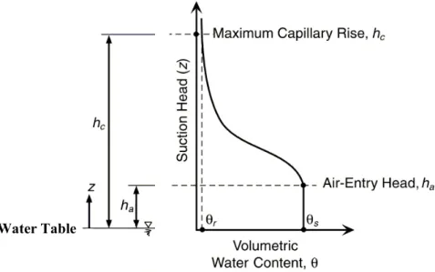
Fig. 3.2: Capillary rise and associated pore water retention in an unsaturated soil profile (Lu and Likos, 2004). ... 30

Fig. 3.3: Schematic classification of flow through porous media, (Bear, 1972) ... 32

Fig. 3.4: A typical water retention curve showing approximate locations of the residual water content , the saturated water content and the air entry pressure . The figure shows also the different zones within a drying cycle. ... 35

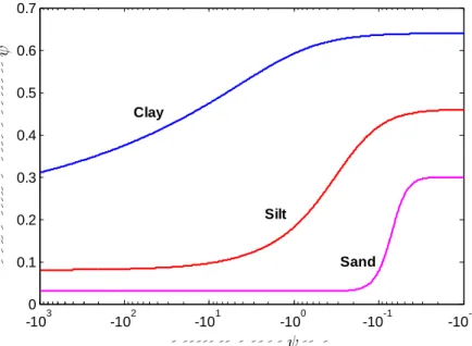
Fig. 3.5: Water retention curves for a clay, silt and sand. ... 36

Fig. 3.6: Effect of the parameter “alpha” of the van Genuchten-Mualem model on the shape of the water retention curve, (alpha variable, n= 2, m=1-1/n). ... 42

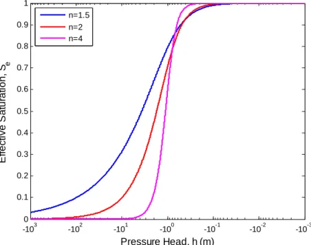
Fig. 3.7: Effect of the parameter n of the van Genuchten-Mualem model on the shape of the water retention curve, (alpha=1 m-1_{, n= variable, m=1-1/n)... 43}

Fig. 4.1 Simplified schematic of the principle iterations in BIGFLOW 3D. ... 46

Fig. 4.2: Schematic of the input/output files in BIGFLOW 3D. ... 48

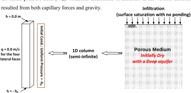
Fig. 4.3: Initial and boundary conditions used in the infiltration test for the different soils. ... 53

Fig. 4.4: Water retention curve for the three porous media used in the simulation. The figures are presented in different scale for the suction head: (a) in logarithmic scale, (b) in linear scale with a zoom taken between 0 and -1m of suction pressure. ... 54

(20)

xiii

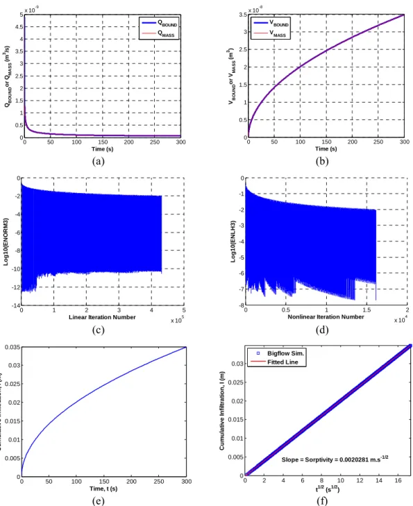
Fig. 4.6: BIGFLOW simulation results for horizontal infiltration case into medium sand (PM1):

(a) Local mass balance: evolution of QBOUND and QMASS. (b) Global volume balance: evolution of

VBOUND and VMASS. (c) Linear iteration convergence. (d) Nonlinear iteration convergence. (e)

Evolution of the cumulative infiltration. (d) Sorptivity determination by fitting a linear regression line to versus data points. ... 57

Fig. 4.7: BIGFLOW simulation results for horizontal infiltration case into fine sand (PM2): (a)

Local mass balance: evolution of QBOUND and QMASS. (b) Global volume balance: evolution of

Fig. 4.8: BIGFLOW simulation results for horizontal infiltration case into Guelph loam (PM3): (a)

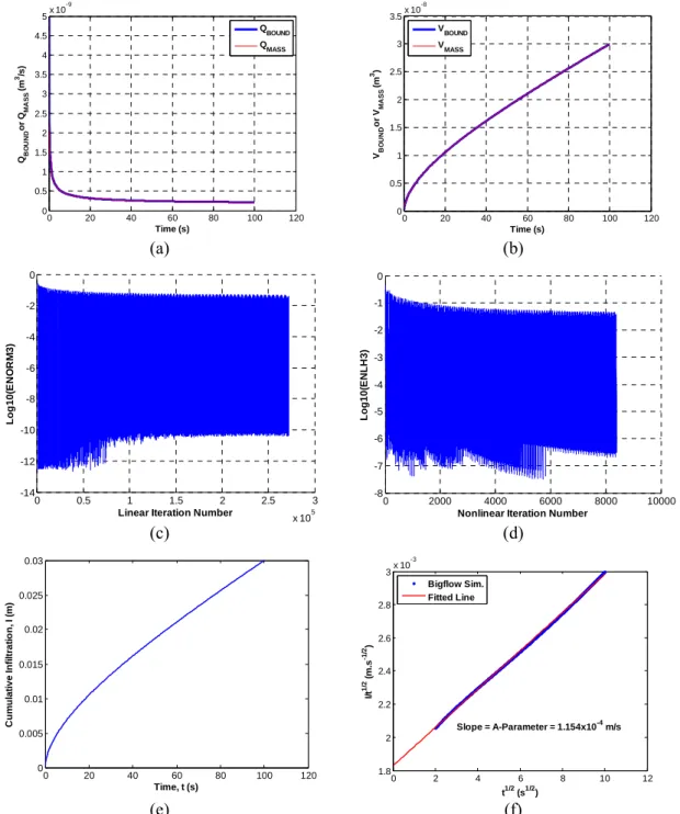
Fig. 4.9: BIGFLOW simulation results for vertical infiltration case into medium sand (PM1): (a)

VBOUND and VMASS vs. time. (c) Linear iteration convergence. (d) Nonlinear iteration convergence.

(e) Evolution of the cumulative infiltration. (d) A-parameter determination by linear fitting of the versus relationship. ... 61

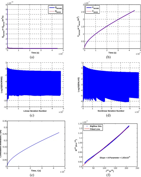
Fig. 4.10: BIGFLOW simulation results for vertical infiltration case into fine sand (PM2): (a)

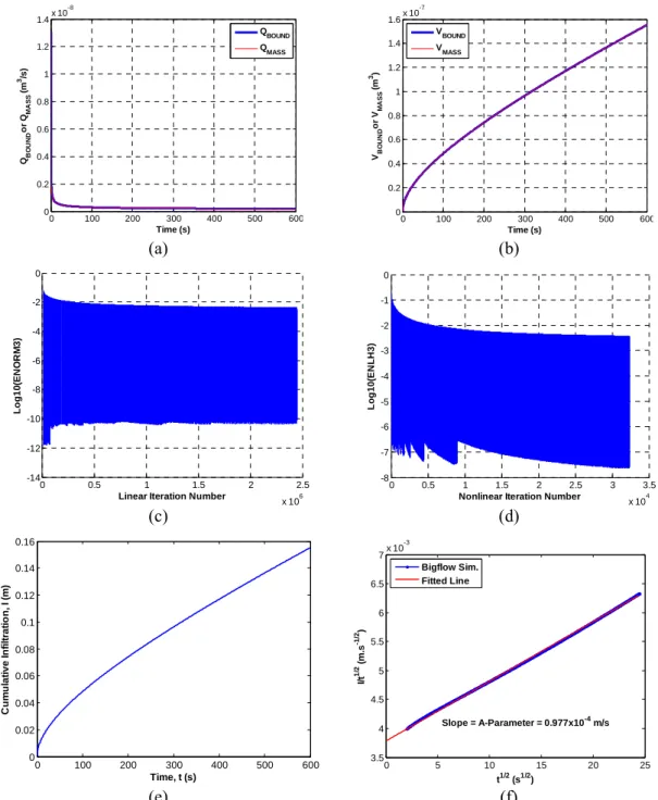
Fig. 4.11: BIGFLOW simulation results for vertical infiltration case into Guelph loam (PM3): (a)

(21)

xiv

Fig. 4.12: Evolution of moisture profile , for the medium sand (PM1); the figure shows a

comparison between the numerical simulation from BIGFLOW (Solid line) and the

quasi-analytical solution of Philip (discrete marks). ... 64

Fig. 4.13: Evolution of moisture profile , for the fine sand (PM2); the figure shows a comparison between the numerical simulation from BIGFLOW (Solid line) and the quasi-analytical solution of Philip (discrete marks). ... 65

Fig. 4.14: Evolution of moisture profile , for the Guelph loam (PM3); the figure shows a comparison between the numerical simulation from BIGFLOW (Solid line) and the quasi-analytical solution of Philip (discrete marks). ... 65

Fig. 5.1: Schematic diagram of the tide machine, soil column and measurement system. ... 68

Fig. 5.2: Photographs of the "sand column" experiment conducted at the IMFT laboratory. Left: sand column with the tensiometers and TDR probes; right: the tide generating machine and its supporting structure (above) and a part of the data acquisition system (below). ... 69

Fig. 5.3: Overflow tank circulation provides a sinusoidal function driving head. ... 70

Fig. 5.4: Left: Schematic of the movable support. Right: Photo of the movable support with the motor axe, rotating arm and the moving overflow tank ... 71

Fig. 5.5: Relationship between the frequency of the electrical power supplied to the motoreductor and the rotation period of the rotating arm. ... 72

Fig. 5.6: Schematic of the rotating arm (dimensions in mm). ... 73

Fig. 5.7: Top: Schematic diagram-side view (Top) and Photo (Below) of the overflow tank. .... 74

Fig. 5.8: Pivot/ Free rotating connection details: (a) schematic details ; (b) cylindrical roller thrust bearing. ... 75

Fig. 5.9: Left: General sand column details (the number and the position of the tensiometers and the TDR probes differs from the actual cases); left: details and dimensions of long column used in the experiments. ... 76

Fig. 5.10: TDR connection: (a) schematic details; (b) fitting picture. ... 77

Fig. 5.11: Tensiometer connection: (a) schematic details; (b) picture. ... 77

(22)

xv

Fig. 5.13: Schematic diagram of the data acquisition system. ... 80 Fig. 5.14: Calibration model of the pressure-transducer named B1T1. The surface represents the

calibration model and the (17) balls represent the calibration points used to find the model

through a multiple linear regression scheme. ... 82

Fig. 5.15: Left: Photos of sand raining method used to fill the 1D sand column with four sieves

and a funnel. Right: photo of the column bottom during the early stage of the filling process. .... 84

Fig. 5.16: The sand column at the end of the filling process. ... 85 Fig. 5.17: Grain size distribution of the sand used in the experiment. ... 86 Fig. 5.18: Photos Schematic of the used constant head permeameter test, the cross-sectional area

and the length of the sand column is and L respectively. ... 88

Fig. 5.19: Constant head permeability test conducted on the sand column to measure the

saturated hydraulic conductivity. Two overflow tanks are attached at the top and bottom of the column ... 90

Fig. 5.20: Photo of the sand column at the end of the imbibitions step (the imposed water table

height is 5mm measured from the bottom of the sand). This photo corresponds to a

steady sate conditions. ... 92

Fig. 6.1: Schema showing the position of the overflow tank in the case of initial condition

application. ... 95

Fig. 6.2: The evolution of the pore water pressure head [ , ] over three time periods at different elevations ( ) along the sand column for relatively high frequency bottom forcing

pressure with the following parameters: 0 = 0.2m, 0 = 0.3m, ! = 573sec (9.55min). ... 99

Fig. 6.3: The evolution of the pore water pressure head [ , ] over three periods at different elevations ( ) along the sand column for relatively low frequency bottom forcing pressure with

the following parameters: 0 = 0.2m, 0 = 0.3m, ! = 6657sec (110.95min). ... 99

Fig. 6.4: The evolution of the total head [" , ] over three time periods at different elevations ( ) along the sand column for relatively high frequency bottom forcing pressure with the

(23)

xvi

Fig. 6.5: The evolution of the total head [" , ] over three time periods at different elevations ( ) along the sand column for relatively low frequency bottom forcing pressure with the

following parameters: 0 = 0.2m, 0 = 0.3m, ! = 6657sec (110.95min). ... 101

Fig. 6.6: Amplitudes of the pore water pressure versus the elevation ( ) along the sand column at

different oscillatory bottom forcing frequencies [ 0 = 0.2m, 0 = 0.3m, ! = variable]. ... 103

different 0 of the oscillatory bottom forcing [ 0 = variable, 0 = 0.5m, ! = 110min]. ... 103

different 0 of the oscillatory bottom forcing [ 0 = 0.2m, 0 = variable, ! = 110min]. ... 104

Fig. 6.9: Phase lag of the pore water pressure versus the elevation ( ) along the sand column at

different oscillatory bottom forcing frequencies [ 0 = 0.2m, 0 = 0.3m, ! = variable]. ... 106

Fig. 6.10: Pressure head profiles at 9 different times separated by !/8; the bottom forcing

parameters are: 0 = 0.2m, 0 = 0.3m and (a) ! = 573sec (9.55min); (b) ! = 6657sec

(110.95min). The red dashed line is the hydrostatic pressure head profile. ... 108

Fig. 6.11: Total head profiles at 9 different times separated by !/8; the bottom forcing

parameters are: 0 = 0.2m, 0 = 0.3m and (a) ! = 573sec (9.55min); (b) ! = 6657sec

(110.95min). The red dashed line is the hydrostatic pressure head profile. ... 108

Fig. 6.12: Total head profiles at (a) !/2 during a falling water table and (b) ! during a rising water table. The presented profiles are for a relatively high frequency bottom

forcing with the following parameters: 0 = 0.2m, 0 = 0.3m, ! = 573sec (9.55min). The

arrows in the figure show the flow direction. The red dashed line is the initial hydrostatic

condition. ... 109

Fig. 6.13: Water table fluctuations [ ] over two time periods. The bottom forcing parameters

are: 0 = 0.2m, 0 = 0.3m and a variable time period ( !) of about 110 min (the blue curve) and

of about 10 min (the red curve). The dashed black curve is the bottom forcing. ... 112

Fig. 6.14: Water table amplitude versus bottom forcing period. [ 0 = 0.2m, 0 = 0.3m, ! = variable]. ... 113

Fig. 6.15: Water table phase lag versus bottom forcing frequency. [ 0 = 0.2m, 0 = 0.3m, ! = variable] ... 114

(24)

xvii

Fig. 6.16: Water table time average versus bottom forcing frequency. [ 0 = 0.2m, 0 = 0.3m, ! = variable] ... 115

Fig. 7.1: Flowchart of the optimization procedure linking the genetic algorithm(GA) to numerical

model (BIGFLOW). ... 121

Fig. 7.2: Observed versus calibrated water table height. The bottom forcing pressure parameters

are: 0 = 0.2m, 0= 0.3m, ! = 1223.95 sec (20.4min). ... 124

Fig. 7.3: Water table amplitude ( ) versus bottom forcing periods ( !). Other bottom forcing

parameters are: 0 = 0.2m, 0= 0.3m; The arrow shows the experiment used for calibration ( ! =

1223.95 s). ... 125

Fig. 7.4: Mean water table height ( ) vs. the time period ( !) of the bottom forcing for the

calibrated SilicaSand. Other bottom forcing parameters are: 0 = 0.5 m, 0= 0.5m. ... 129

Fig. 7.5: Root mean square of the water table height (& ) vs. the time period ( !) of the bottom

forcing for the calibrated SilicaSand. Other bottom forcing parameters are: 0 = 0.5 m, 0=

0.5m. ... 129

Fig. 7.6: Mean water table height ( ) vs. the time period ( !) of the bottom forcing for the

Guelph Loam. Other bottom forcing parameters are: 0 = 0.5 m, 0= 0.5m. ... 130

Fig. 7.7: Root mean square of the water table height (& ) vs. the time period ( !) of the bottom

forcing for the Guelph Loam. Other bottom forcing parameters are: 0 = 0.5 m, 0= 0.5m. .... 130

Fig. 7.8: Mean water table height ( ) vs. the time period ( !) of the bottom forcing for different ' values. Other bottom forcing parameters are: 0 = 0.5 m, 0= 0.5m. ... 131

Fig. 7.9: Root mean square of the water table height (& ) vs. the time period ( !) of the bottom forcing for different ' values. Other bottom forcing parameters are: 0 = 0.5 m, 0= 0.5m. ... 132

Fig. 7.10: Mean water table height ( ) vs. the time period ( !) of the bottom forcing for

different values. Other bottom forcing parameters are: 0 = 0.5 m, 0= 0.5m. ... 133

Fig. 7.11: Root mean square of the water table height (& ) vs. time period ( !) of the bottom

(25)

xviii

Fig. 7.12: Mean water table height ( ) vs. the time period ( !) of the bottom forcing for

different ( values. Other bottom forcing parameters are: 0 = 0.5 m, 0= 0.5m. ... 135

Fig. 7.13: Root mean square of the water table height (& ) vs. time period ( !) of the bottom forcing for different ( values. Other bottom forcing parameters are: 0 = 0.5 m, 0= 0.5m. ... 135

Fig. 9.1: Photo of the 2D experiment; the photo show also the tide machine used to generate the

(26)

(27)

xix

List of Tables

Table 3.1 : Models of water retention curve ... 37

Table 4.1 : Hydraulic characteristics of porous media used in the simulation ... 55 Table 4.2: Sorptivity values comparison ... 60

Table 4.3 : Comparison between the A-parameter and ) values ... 64

Table 6.1 : Summary of the experiments driving head parameters (the experiments marked by the red color were excluded from the analysis due to time drift problem) ... 97 Table 7.1 : The upper and lower bounds of soil hydraulic parameters (applied in the optimization problem) and measured versus calibrated parameter values. ... 123

(28)

(29)

I

Introduction (en français)

1. Nature et contenu de l'étude

Les interactions entre écoulements superficiels et souterrains concernent un large éventail d'applications. Ces interactions se produisent dans les milieux aquatiques d'eau douce et d'eau salée, en milieux naturels et artificiels. On les rencontre par exemple dans les plages, les berges de fleuves, les digues poreuses et les barrages en terre et enrochements (Fig. F.1).

Les fluctuations dans les eaux de surfaces affectent les eaux souterraines auxquelles elles sont connectées. Les fluctuations temporelles qui se produisent dans les eaux de surface peuvent être d'origine naturelle ou anthropique : précipitations, crues, oscillations tidales (marées), ondes de surface, lâchers de barrages, etc. (Boutt, 2010).

Dans cette thèse, on s'intéresse à l'hydrodynamique souterraine des plages en zone côtière. Il est reconnu que les écoulements souterrains en zone côtière influencent le transport de sédiments et les processus morphologiques (érosion et dépôt) notamment dans la zone de jet de rive (Baird and Horn, 1996, Jeng et al., 2005b).3_{Les eaux}

souterraines côtières contrôlent aussi les conditions biologiques, le cycle des nutriments, et les transferts de contaminants au voisinage de la surface libre de la nappe côtière (Chen and Pinder, 2011, Hinz, 1998). Enfin, les écoulements souterrains affectent la stabilité des structures bâties sur des sols sableux près des plages (Nielsen, 1990).

(30)

II

Fig. F.1: Photographies illustrant les couplages entre écoulements superficiels et souterrains en hydrologie et en hydrodynamique côtière. En haut à gauche: cas d'une plage de sable dont la nappe est couplée aux fluctuations du niveau de la mer. En haut à droite: cas d'une rive ou d'un îlot de sable et galets en milieu fluvial. En bas à gauche: cas d'un barrage en terre et enrochements, avec son lac-réservoir dont le niveau peut fluctuer. En bas à droite: cas d'une île de sable artificielle, "Palm beach", construite récemment à Dubaï.

En hydrodynamique côtière (plages) on peut distinguer deux types de "forçages" oscillatoires :

• les phénomènes basse fréquence ou ondes longues, de type "tidal" : cette catégorie désigne ici les ondes de marée de période 12h ou 24h, ou encore, d'autre phénomènes basse fréquence mais de périodes parfois plus courte (seiches), ou au contraire, les fluctuations non stationnaires de plus longue période (marées d'équinoxes, etc.);

• les phénomènes haute fréquence ou ondes courtes : cette catégorie désigne ici les ondes complexes et déferlantes, les processus de flux et reflux dans la zone de jet de rive (zone de swash), ainsi que les processus d'érosion (transports solides) qui accompagnent ces phénomènes en bord de plage dans la zone de swash.

(31)

III Dans cette thèse, on se concentre sur les oscillations "tidales" au sens défini plus haut. Plus précisément, on s'intéresse aux écoulements oscillatoires à l'intérieur d'un milieu poreux partiellement saturé / non saturé (plage) sous l'action d'oscillations tidales du niveau d'eau dans un milieu ouvert environnant (océan, mer, lac, estuaire), lequel est connecté au massif poreux. Dans ce travail, le forçage tidal des eaux souterraines sera représenté, ou idéalisé, par des oscillations quasi-statiques du niveau d'eau dans un réservoir de pleine eau connecté au domaine poreux (ceci sera précisé par la suite).

2. Objectifs et méthodologie

L'objectif général de cette thèse est d'améliorer la compréhension des phénomènes d'écoulements oscillatoires ou rapidement variés en milieux poreux partiellement saturés et/ou non saturés (plages de sable, digues portuaires, barrages en terre, berges fluviales, estuaires, etc.).

Plus particulièrement, le but de cette thèse est d'étudier les interactions entre eaux souterraines et eaux de surface, en prenant en compte tant la zone saturée que la zone non saturée, et donc, en incluant dans l'étude non seulement la surface libre de la nappe mais aussi la zone capillaire sus-jacente. Les résultats attendus concernent la réponse hydrodynamique du milieu poreux (plage) lorsqu'il est soumis à des oscillations périodiques du niveau de la mer (le forçage "tidal" défini plus haut).

Pour atteindre ces objectifs, trois types d'approches sont mises en œuvre :

• I). Expériences de laboratoire sur des colonnes verticales, avec une machine à marée pour générer des oscillations tidales imposées par le bas de la colonne, et en utilisant des tensiomètres pour mesurer aussi bien les pressions positives dans la zone saturée que les succions dans la zone non saturée (entre autres méthodes).4

• II) Simulations numériques des écoulements oscillatoires en milieux poreux partiellement saturés / non saturés au comportement hydrodynamique fortement

4_{Une autre expérimentation sur une maquette bi-plaque 2D, avec sable de plage inclinée, a été récemment}

(32)

IV non linéaire. La méthode numérique est celle implémentée dans le code BIGFLOW

(volumes finis 3D implicite, avec une méthode itérative point fixe ou Picard pour le problème non linéaire). De plus, une méthode de calage automatique a été implémentée afin d'optimiser les paramètres hydrodynamiques du sol expérimental (algorithme génétique).5

• III) Développement et mise en œuvre de solutions quasi-analytiques pour le calcul des écoulements oscillatoires dans une colonne de sol partiellement saturée / non saturée. Ceci inclut en particulier une nouvelle approche multi-front, basée sur une série de généralisations de l'approche de Green et Ampt des écoulements piston, et conduisant à des systèmes d'Equations Différentielles Ordinaires non linéaires et non autonomes, qui permettent d'obtenir rapidement les solutions de l'équation de Richards en présence de forçages temporels oscillatoires et fortement variables.

3. Plan de la thèse

Cette thèse est composée de neuf chapitres comme suit.

• Le Chapitre 1 (ce chapitre introductif) présente une vue d'ensemble du travail, ses objectifs, les méthodes utilisées, et le plan du mémoire de thèse.

• Le Chapitre 2 présente une revue de la littérature sur l'hydrodynamique souterraine des plages de sable en réponse aux fluctuations d'origine tidale.

• Le Chapitre 3 introduit les concepts de base et les équations régissant les écoulements en milieux poreux non saturés, ou partiellement saturés: équations de Darcy, de conservation de masse, et de Richards. Les relations constitutives (θ(h), K(h)) requises pour résoudre l'équation de Richards sont également analysées (paramétrisation): à partir du modèle de van Genuchten / Mualem, une étude paramétrique est effectuée, et une interprétation physique des paramètres est

5_{De plus, le code de calcul B}_IG_F_LOW_{a été amélioré de la façon suivante au cours de ce travail : on a}

implémenté et testé le cas de conditions limites temporellement variables (signaux de pression); on a amélioré et automatisé les visualisations spatio-temporelles des champs de pression et de teneur en eau; et l'on a conçu une nouvelle interface MATLAB interface à menus déroulants, comme alternative à l'interface

(33)

V développée, en particulier, l'échelle de longueur capillaire (voir également l'échelle de

temps gravitaire dans le chapitre suivant).

• Le Chapitre 4 commence par présenter une revue du modèle numérique BIGFLOW,

solveur de l'équation de Richards, utilisé dans une partie de cette thèse pour la simulation des écoulements oscillatoires en milieu poreux à saturation variable. Outre les aspects numériques (grille volumes finis 3D, domaine de calcul, conditions limites, fonctions auxiliaires non linéaires) -- les interfaces et processeurs graphiques du code sont aussi présentés. Enfin, on développe des tests de validation et de calage du code en exploitant certains concepts de la théorie de l'infiltration. Ceux-ci permettent, via des expériences numériques, de préciser l'interprétation physique des effets capillaires (sorptivité "S") ainsi que la compétition gravité/capillarité (temps gravitaire "tGRAV").

• Le Chapitre 5 contient une description détaillée du montage expérimental de la colonne de sol instrumentée (milieu poreux étudié à l'échelle de Darcy) ainsi que du système hydraulique et mécanique appelé "machine à marées". Ce chapitre discute aussi des méthodes de calage des capteurs (particulièrement les tensiomètres), ainsi que le protocole expérimental de remplissage de la colonne de sol. Les propriétés hydrodynamiques du sol de la colonne sont en partie mesurées directement, et en partie calées (sur ce dernier aspect, voir le chapitre 7).

• Le Chapitre 6 présente les résultats expérimentaux obtenus sur la colonne de sol soumise à des oscillations via la machine à marées. Les résultats sont présentés en termes de signaux de pression interstitielle, pression totale (ou charge hydraulique), et cote de la surface libre de la nappe. On présente aussi les résultats en termes de profils verticaux de pression ou de charge. On étudie les déphasages, atténuations et structures temporelles des différents signaux, pour tout une gamme de paramètres expérimentaux (période tidale, amplitude, niveau d'eau statique). Ces résultats expérimentaux seront étendus à une gamme plus large de paramètres par simulations (cf. Chapitre 7 - analyses étendues en fonction de la fréquence de forçage).

(34)

VI

• Le Chapitre 7 a comme but d'étendre numériquement les résultats expérimentaux, c'est-à-dire, d'examiner les effets du forçage oscillatoire en dehors de la gamme des paramètres expérimentaux (gamme de fréquences, types de sols). On commence par procéder à un calage optimal des paramètres du sol à l'aide d'un algorithme génétique (ceci revient à résoudre un problème inverse pour identifier certains paramètres hydrodynamiques). Pour étudier la performance du calage, on cale les paramètres sur une seule expérience (fréquence ω1 donnée), puis on tente de reproduire par

simulation les résultats d'autres expériences (fréquences ω2, ω3, etc.). On présente

ensuite une étude paramétrique étendue, visant à analyser la réponse de la nappe à une sollicitation en fréquence. Un des objectifs est de déceler une fréquence caractéristique permettant de distinguer deux régimes hydrodynamiques, haute fréquence et basse fréquence, selon le type de sol.

• Le Chapitre 8 présente une approche théorique quasi-analytique de type "multi-front", qui permet de modéliser efficacement la réponse hydrodynamique d'une colonne de sol à un forçage fortement variable et/ou oscillatoire (temporel).6

L'approche multi-front donne une famille de modèles à N fronts, généralisations successives de l'approche "écoulement piston" de Green et Ampt, adaptée au problème des oscillations tidales. Tout d'abord, un modèle à front unique est développé (Green-Ampt "inversé"). Ce modèle à 1 front est ensuite généralisé à 2 fronts puis N fronts. La paramétrisation du modèle est définie en termes des courbes non linéaires de teneur en eau et de conductivité hydraulique du sol (θ(h), K(h)). La performance du modèle multi-front est discutée et testée en utilisant des solutions fines de l'équation de Richards par le code volumes finis BIGFLOW, comme base de

comparaison.

• Le Chapitre 9 contient les conclusions sur les différentes parties du travail (expérimentales, numériques, théoriques), ainsi que les perspectives et recommandations en vue d'extensions futures de ce travail de recherche.

(35)

1

Chapter 1: Introduction

Chapter 1 Introduction

1.1 Nature and extent of the study

Surface/subsurface flow interactions concern a wide range of applications. Such interaction is found in both fresh and salt water environments and also in natural and man-made structures. This interaction encountered for example in beaches, river banks, porous dykes and earth dams (Fig. 1.1).

Surface water fluctuations strongly influence adjacent groundwater. Variations in surface water can arise from many natural and anthropogenic sources including precipitation and flood events, tidal oscillation, wave-induced displacement, dam releases, and associated reservoir drawdown (Boutt, 2010).

In this thesis, we are interested in beach groundwater hydrodynamics. Coastal groundwater flow has been recognized to influence the sediment transport and morphological processes like erosion and accretion in the swash zone (Baird and Horn, 1996, Jeng et al., 2005b), and to control the biological conditions, nutrient cycling and contaminant movement near the water table (Chen and Pinder, 2011, Hinz, 1998). Coastal groundwater flow also affects the stability of the structures founded on soils and sands near beaches (Nielsen, 1990).

(36)

2 Fig. 1.1: Photographs illustrating the coupling between surface and subsurface flows in hydrology and coastal hydrodynamics: the top left photograph illustrates the case of a sand beach with groundwater coupled to sea level fluctuations; the top right illustrates the case of a sand/gravel river bank or island; the bottom left shows an earth-fill dam with its reservoir lake shown at left; the bottom right is the artificial sand island "Palm Beach" designed recently in Dubai.

In the context of beach and coastal hydrodynamics, two main types of periodic “forcing” are encountered:

• low frequency / long tidal waves: this category designates slow "tidal" waves with long periods, e.g. 12h or 24h, as well as other phenomena with possibly somewhat shorter periods (such as "seiches");

• high frequency / short waves: this item designates complex nonlinear surface waves occurring in coastal areas; they may involve overspill phenomena (breaking waves), and run up/run down processes in the swash zone, as well as erosion processes (solid transport).

(37)

3 In this thesis, we focus on studying the effect of "tidal" oscillations taking place in porous bodies (partially saturated/unsaturated porous media). The tidal forcing of groundwater will be approximated, or idealized, by quasi-static oscillations of water levels in an open water reservoir adjacent to the porous medium.

1.2 Thesis objectives and methodology

The general objective of this thesis is to further advance the current understanding of oscillatory flows in porous bodies (sand beaches, harbor dykes, earth dams, river banks, estuaries, etc.).

More specifically, the aim in this thesis is to study beach groundwater /surface water interactions, taking into account both the saturated and unsaturated zones (including water table and capillary zone) under the effect of tidal forcing. The expected result should be a better understanding of the hydrodynamic response of the porous medium (the beach and its groundwater) when it is submitted to periodic tidal oscillations of sea water levels.

To fulfill the above objectives, three types of approaches are used:

• Laboratory experiments on vertical sand columns, with a tide machine to force the water table oscillations at the bottom of the column, and tensiometers to measure both positive pressures and suctions, among other measurement methods.7

• Numerical simulations of oscillatory water flow in partially saturated / unsaturated porous media with strongly non-linear behavior in porous media. The numerical simulation method is implemented in the BIGFLOW code (implicit 3D finite volumes,

with fixed point or Picard iterations for the nonlinear problem). In addition, an

7_{Another experiment involving a 2D slab of soil with a sloping sand beach has been recently constructed}

(38)

4 automatic calibration method was implemented to optimize the hydrodynamic parameters of the experimental soil based on a Genetic Algorithm.8

• Quasi-analytical solutions of oscillatory flows in a partially saturated/unsaturated porous column. This includes novel multi-front approaches, which generalize the Green-Ampt piston flow approach, leading to nonlinear differential equations.

It is worth noting that most of this thesis manuscript focuses on the effect of oscillations on homogeneous soils. However, other analyses on multilayered media were also presented (see Appendix E)

1.3 Thesis outline

This thesis is composed of nine chapters as follows:

• Chapter 1 (this chapter) is an introductory chapter which provides an overview of the research study, its objectives, methodology and the outline of the dissertation.

• Chapter 2 presents a review of the relevant scientific literature on beach groundwater hydrodynamics in response to fluctuations in open water bodies.

• Chapter 3 introduces the basic definitions and the governing equations used to model variably saturated flow numerically, taking into account both saturated and unsaturated zones. The Darcy equation, mass conservation equation, and the resulting Richards equation (Partial Differential Equation) are presented. The constitutive relationships [ , ' ] required to solve the Richards equation are then reviewed. The van Genuchten / Mualem model is introduced; a parametric study is conducted, and a physical interpretation of the model parameters is given (capillary length scale).

• Chapter 4 provides a review of the numerical code used in this thesis to simulate variably saturated flow in porous media (BIGFLOW). The main code, the pre- and

post-processors, the computational domain, and the boundary conditions, are briefly

8_{Furthermore, the numerical code B}_IG_F_LOW_{was enhanced for this study in the following ways: the case of}

time varying Boundary Conditions was implemented and tested (input pressure signals); the 2D/3D space-time visualizations of water contents and pressure outputs was enhanced and automatized; and a new MATLAB interface was designed as an alternative to the existing Python interface.

(39)

5 discussed. Finally, a validation test for the numerical procedure is proposed and analyzed through the concepts of the infiltration theory; Physical interpretations of the results in terms of hydraulic conductivity, capillary effects, sorptivity and gravitational time scale are also given.

• Chapter 5 contains a detailed description of the experimental setup of the Darcy-scale soil column and the associated hydro-mechanical system (tide machine). The chapter also discusses the methods used to calibrate the measurement sensors (especially tensiometers), and to fill and pack the sand into the column. The properties of the sand (used in the experiment) obtained from various measurements are presented (see also the calibration section in chapter 7).

• Chapter 6 presents the experimental results of the oscillatory flow in the porous column / tide machine system. The results are presented in terms of the signals of pore water pressure, total pressure, and water table elevation, together with the profiles of pressure and total head. The attenuation, phase lag, and non harmonic structures of the different signals, are also discussed. Preliminary analyses and interpretations of the experimental results, based on the available range of forcing parameters (tidal period, tidal amplitude, and static level) are conducted. These experimental results are re-analyzed numerically in Chapter 7 below (extended analyses).

• Chapter 7 extends the experimental study numerically, in order to examine the effect of oscillatory forcing outside the available range of the physical experiment (frequencies, type of soil). We start by implementing an optimal calibration of the numerical model using a Genetic Algorithm (this is equivalent to solving an inverse problem for the hydrodynamic parameters of the soil). Then we provide an extended numerical parametric study of the frequency response of the water table. One of the objectives is to identify a characteristic frequency separating low and high frequency regimes.

(40)

6

• Chapter 8 provides the details of the semi-analytical multi-front approach developed to model the water table response to periodic forcing in porous columns.9 The multi-front approach is the result of a series of generalizations of the Green-Ampt piston flow approach. First, a single front model is developed based on an "inverted" version of the classical Green-Ampt infiltration model, with a sharp "wetting front" separating the fully saturated and the totally dry regions. The model is then further extended to two fronts (N=2), and more generally to multi-front (N ≥ 2). The parametrization of the model is defined in terms of the nonlinear water content and conductivity curves of the soil [ , ' ]. The performance of the multi-front models is discussed and tested using a refined finite volume solution of the non linear Richards equation (BIGFLOW code) as a basis for comparisons.

• Chapter 9 comprises the major conclusions for the whole thesis, together with recommendations and perspectives for future research (outlook).

In addition to the above chapters, this thesis includes the following appendices:

• Appendix A: deals with the effect of the acceleration (Eulerian and inertial accelerations) on the validity of using Darcy’s equation.

• Appendix B: gives a comparison between our experiment results conducted on the sand column and the analytical model of Nielsen and Perrochet (2000) (complex effective porosity).

• Appendix C: provides preliminary optical measurements of the water content [ , ] using CCD camera.

• Appendix D: contains numerical simulations on homogeneous column under tidal forcing (a conference paper).

• Appendix E: contains additional simulation tests and analyses on a two-layered medium under tidal forcing (a conference paper).

(41)

7

Chapter 2: Literature Review

Chapter 2 Literature Review

2.1 Introduction

This chapter presents a review of the relevant scientific works on beach groundwater hydrodynamics in response to surface water fluctuations mainly due to tidal forcing. The chapter also presents the recent study involving vertical flows and capillary effects in the groundwater dynamic models.

(42)

8

2.2 Overview

Beach groundwater dynamics has been recognized to influence the morphological processes and sediment transport (erosion and accretion) of the swash zone (Baird and Horn, 1996, Jeng et al., 2005b) and to control the biological conditions, nutrient cycling and contaminant movement near the water table (Chen and Pinder, 2011, Hinz, 1998). It also affects the stability of the structures founded on soils and sands (Nielsen, 1990).

To understand and manage the behavior of coastal aquifers, it is required to accurately predict the dynamic groundwater hydraulics.

Beach groundwater hydrodynamics are a result of combined influence from tides and wave forcing. This thesis and consequently this literature review are concerned mainly with tidal forcing effects.

Fig. 2.1 shows a descriptive overview (and terminology) of the forcing at a coastal boundary. In this figure, the MSL is Mean Sea Level. The Still Water Surface (SWS) is the surface that would be measured in the absence of waves (the surface that oscillates with the tide only).The Mean Water Surface (MWS) is the water level, averaged over several wave periods, that indicates the set-up due to wave action. The Shoreline (SL) is defined as the intersection of the MWS with the sand surface. RL is the wave run-up limit. UENV and LENV are the upper and lower envelope boundaries of the water table oscillations. η+ is the total water table overheight as a result of sea forcing.

(43)

9

2.3 Beach groundwater behavior under tidal forcing

In this section, the behavior and observations of the beach groundwater under the effect of tidal oscillations in the adjacent water body are highlighted and summarized as following:

• Observations from the field and laboratory experiment show that the coastal aquifer responds to the tidal forcing which manifested as fluctuations in the water table of the adjacent aquifer (Li et al., 1997a) and also as fluctuations of the pore water pressure of the aquifer below the water table (Li et al., 2000a).

• The slope of the fluctuating water table is not flat, however the water table sloping seaward on a falling tide and landward on a rising tide and is generally steeper on a rising tide than on a falling tide (Horn, 2006, Raubenheimer et al., 1999).

• The groundwater fluctuations, as induced by the oceanic oscillations, affect water and mass exchange between the aquifer and ocean (Li et al., 2000a).

• The water table fluctuations propagate in the landward direction. (Nielsen et al., 1997) stated that the tidal oscillations vanished within 50m or so from the high water mark in an unconfined aquifer. However, their influence can be considerable up to few hundred meters inland from the shore (Lanyon et al., 1982, Li et al., 2000a). The propagation of these fluctuations is influenced primarily by oscillation frequency, modified by the aquifer parameters, vertical flow and capillarity (Horn, 2006).

• The amplitude of the tidal water table fluctuations is clearly attenuated in the landward direction (Raubenheimer et al., 1999, Baird et al., 1998, Nielsen, 1990).

• The time averaged of the fluctuating water table height may stand significantly above mean sea level (Raubenheimer et al., 1999, Turner et al., 1997). This is often referred to in the literature as an over-height or super-elevation. The lower the beach face slope and/or finer the sand of which it is composed, the higher coastal groundwater is anticipated to stand above mean sea level (Turner et al., 1997, Kang and Nielsen, 1996).

(44)

10

• Tidal water table fluctuations were asymmetrical in time as the beach fills more rapidly than it drains. In this context, (Turner et al., 1997) stated that: “the physical explanation for the significance of a sloping coastal boundary is straightforward to comprehend. Water can infiltrate vertically into the beach face during the flooding tide, but must seep essentially horizontally through the beach during the ebbing tide. In simple terms, a beach will 'fill' more easily that it can 'drain'. It is clear that a sloping beach face favors ocean inflow, implying a tendency for net super-elevation of the coastal water table and an accompanying skewness of the time variation for tidal water table fluctuations”. It was observed also that the asymmetry increases in the landward direction (Horn, 2006).

• Water table oscillations have been shown to lag behind tidal oscillations. For a given geometry the lag in water table response is due to the hydraulic conductivity of the beach sediment. This lag increases in the landward direction (Horn, 2006).

• Decoupling between the water table and offshore water level occurs on fine-grained beaches near low tide (Turner, 1993b). In reality, across a low gradient beach face the water table typically decouples during tidal ebb, resulting in the formation of a seepage face that continues to increase in vertical extent through the falling tide (Turner et al., 1997).

• Beaches with low water table tend to accrete and beaches with high water table tend to erode (Grant, 1948, Li et al., 1997a, Baird et al., 1998).

Furthermore, the following is a summary of the behavior of the capillary effect on the coastal groundwater dynamics

• The capillary fringe significantly influence the water table dynamics specially for fine soils (Horn, 2006, Hinz, 1998, Li et al., 1997a, Li et al., 2000a); and has a considerable effects on the exchange of water between the ocean and the coastal aquifer (Horn, 2006).

(45)

11

• In the presence of capillary fringe, water table fluctuations propagate faster and decay more slowly (Nielsen and Turner, 2000, Cartwright et al., 2004).

• Capillarity effects provide a mechanism for the propagation inland of high-frequency sea level oscillations (Li et al., 1997a). It is observed also, that capillarity affects water table dynamics over a wider range of frequencies, including the tidal frequency (Nielsen and Perrochet, 2000a).

2.4 Beach groundwater modeling under tidal forcing

Many models have been developed to predict the groundwater response to periodic forcing in the adjacent water body (Baird et al., 1998, Kang and Nielsen, 1996, Nielsen, 1990, Raubenheimer et al., 1999, Song et al., 2007, Teo et al., 2003, Xia et al., 2010).

By scanning relevant works on this topic, most beach groundwater fluctuations models in coastal aquifer are based on the Boussinesq equation. Other models apply modification on Boussinesq equation to account for vertical flow and capillary effects. On the other hand, models based on the numerical solution of the Richards equations are also available. The following sub-sections briefly explore these models.

2.4.1 Partially saturated/unsaturated flow model with capillary effects:

Richards equation

The Richards equation is a standard, frequently used approach for modeling flow in variably saturated/unsaturated porous media (Miller et al., 2006). It can be used with no need to modifications to simulate beach groundwater dynamics under tidal forcing including flows in the unsaturated zone and thus it takes into accounts vertical flows and the capillary effects.

Here we briefly introduce Richards equation (more details in chapter 3) which was formulated by Lorenzo A. Richards in 1931 (Richards, 1931). Richards equation is

(46)

12 obtained by combining Darcy’s law with the mass conservation or continuity equation, under the assumption that the air phase remains at constant (atmospheric) pressure and the water phase is incompressible. It can be expressed as follows (mixed form of Richards Equation [( , ) form]):

* , +,

* div 0' , +, grad 4 56 ∙ +, 8 Eq. 2.1

where:

• , +, : is the volumetric water content; it is function of the pressure head and can vary spatially.

• ' , +, : is the hydraulic conductivity tensor, a symmetric second rank tensor. It is function of the pressure head and can vary spatially.

• 56: is the normalized gravitational vector; 56 95,/|5|, (|5| 9.81m/s@_). • +,: is the point coordinate vector.

The water retention curve, , and the hydraulic conductivity characteristic, ' are soil dependent hydraulic properties that have to be determined in order to model water flow by means of the Richards’ equation. Many functional models were considered in the literature for these nonlinear curves. Richards' equation is highly nonlinear and therefore it is solved by employing numerical methods (for example: Finite element methods, Finite volume methods and Finite difference methods).

Detailed discussion on Darcy’s equation, Richards equation and the corresponding

constitutive relationship [ and ] are presented in the next chapter [see section