From AADL to Timed Abstract State Machines: A Verified Model Transformation
28
0
0
Texte intégral
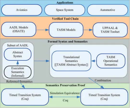
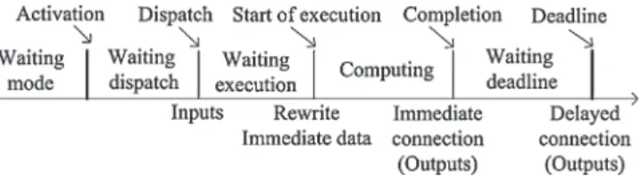
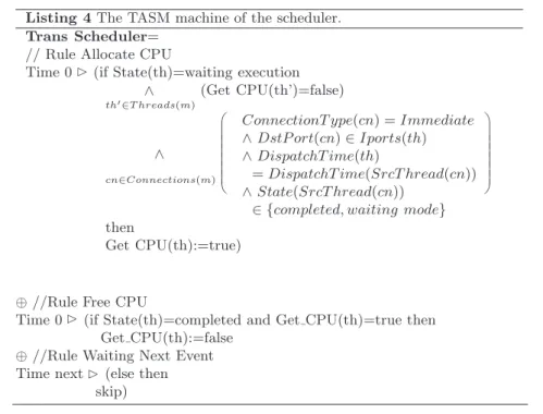
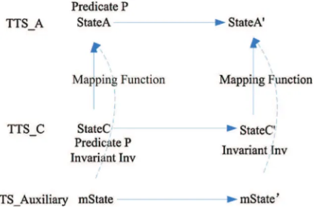
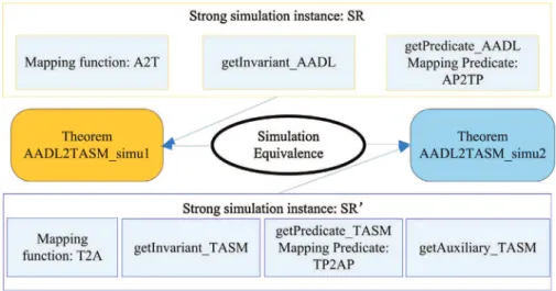
Figure
+6
Documents relatifs
