Science Arts & Métiers (SAM)
is an open access repository that collects the work of Arts et Métiers Institute of
Technology researchers and makes it freely available over the web where possible.
This is an author-deposited version published in: https://sam.ensam.eu
Handle ID: .http://hdl.handle.net/10985/19675
To cite this version :
A. SANSICA, Y. OHMICHI, Jean-Christophe ROBINET, A. HASHIMOTO - Laminar supersonic
sphere wake unstable bifurcations - Physics of Fluids - Vol. 32, n°12, p.1-18 - 2020
Any correspondence concerning this service should be sent to the repository
Administrator : [email protected]
Laminar
supersonic sphere wake
unstable
bifurcations
A. Sansica,1,a) Y. Ohmichi (大道勇哉),1 J.-Ch. Robinet,2 and A. Hashimoto (橋本敦)1
AFFILIATIONS
1Japan Aerospace Exploration Agency, Chofu Aerospace Center, 7-44-1 Jindaiji-Higashi, Chofu, Tokyo 182-8522, Japan 2DynFluid Laboratory, Arts et Métiers/CNAM, 151 Bd. de l’Hopital, Paris 75013, France
a)Author to whom correspondence should be addressed:[email protected]
ABSTRACT
The laminar sphere unstable bifurcations are sought at a Mach number ofM∞= 1.2. Global stability performed on steady axisymmetric base flows determines the regular bifurcation critical Reynolds number atReregcr =650, identifying a steady planar-symmetric mode to cause the loss of the wake axisymmetry. When global stability is performed on steady planar-symmetric base flows, a Hopf bifurcation is found atReHopfcr = 875 and an oscillatory planar-symmetric mode is temporally amplified. Despite some differences due to highly compressible effects, the supersonic unstable bifurcations present remarkably similar characteristics to their incompressible counterparts, indicating a robust laminar wake behavior over a large range of flow speeds. A new bifurcation for steady planar-symmetric base flow solutions is found aboveRe > 1000, caused by an anti-symmetric mode consisting of a 90○ rotation of the dominant mode. To investigate this reflectional symmetry breaking bifurcation in the nonlinear framework, unsteady nonlinear calculations are carried out up toRe = 1300 and dynamic mode decomposition (DMD) based on the combination of input data low-dimensionalization and compressive sensing is used. While the DMD analysis confirms dominance and correspondence in terms of modal spatial distribution with respect to the global stability mode responsible for the Hopf bifurcation, no reflectional symmetry breaking DMD modes were found, asserting that the reflectional symmetry breaking instability is not observable in the nonlinear dynamics. The increased complexity of the wake dynamics atRe = 1300 can be instead explained by nonlinear interactions that suggest the low-frequency unsteadiness to be linked to the destabilization of the hairpin vortex shedding limit cycle.
NOMENCLATURE
CFL Courant–Friedrichs–Lewy number
CL lift coefficient
DMD dynamic mode decomposition
D∗s dimensional sphere diameter
E total energy
Lsep base flow separation length
M∞ inflow Mach number
PS planar-symmetric
PSD power spectral density
q conservative variables’ state vector
qb base flow conservative variables’ state vector
q′ perturbation conservative variables’ state vector ˆq eigenfunction conservative variables’ state vector
Re Reynolds number
ReHopfcr Hopf bifurcation critical Reynolds number Reregcr regular bifurcation critical Reynolds number St Strouhal number, non-dimensional frequency
t time
[u, v, w]T streamwise, transversal, and vertical velocities [ux,ur,uθ]T streamwise, radial, and azimuthal velocities [x, y, z]T streamwise, transversal, and vertical coordinates
ΔT Krylov time step
Δt integration time step
λ complex eigenvalue
ρ density
σ growth rate
σNL growth rate obtained from nonlinear calculations
I. INTRODUCTION
For many engineering applications, the appearance of large-scale unsteadiness represents a design operability limiting factor. The increase of drag and flow-induced vibrations consequent to the unsteadiness onset are not only detrimental for the overall perfor-mances but can eventually lead to structural failure due to fatigue. Fundamental studies on three-dimensional (3D) unsteady dynam-ics associated with axisymmetric bodies, like a sphere, have shown been to be physically relevant to understand more complex con-figurations, such as launcher after-bodies or re-entry capsules. The incompressible behavior of the space-time dynamics of a flow past a sphere has been well documented in the past both experimentally1–5 and numerically.6–14 While the interest of the scientific commu-nity for the incompressible regime is still very high and numerous studies have been recently done,15–20very limited information exists regarding the effects of compressibility, especially at supersonic speeds.
The scientific community currently seems to agree on the sta-bilizing effect of the Mach number (M∞ = U∞∗/c∗∞ withU∞∗ and c∗∞being the dimensional free-stream velocity and speed of sound, respectively) both at subsonic and supersonic speeds for sphere wakes21–25and other flow configurations as thin wakes26and bound-ary layers on rotating disks.27The first (pitchfork or regular) and secondary (supercritical Hopf) unstable bifurcations for an incom-pressible flow past a sphere are responsible for the loss of spatial axisymmetry and for causing the flow to become unsteady, respec-tively. Although they are seen to persist in the compressible regime, the corresponding critical Reynolds numbers move toward higher values for increasing Mach number, indicating its stabilizing effect on the wake dynamics. However, no unstable bifurcations at super-sonic speeds were found in the Reynolds number (Re = U∞∗D∗s/ν∗∞ with ν∗∞being the dimensional free-stream kinematic viscosity and D∗s being the dimensional sphere diameter) range considered (Re <600), and the flow system was shown to be globally stable and, more precisely, temporally steady and spatially axisymmetric. Evi-dence of the existence of unstable bifurcations in the supersonic regime was recently given in a set of direct numerical simulations at higher Reynolds numbers by Nagataet al.,23who found the flow to first lose its spatial axisymmetry and then become unsteady via the shedding of hairpin vortices downstream of the sphere, like for its subsonic counterpart. The experiments of Nagataet al.28at free-flight conditions examined schlieren visualizations of a sphere at 0.9 <M∞ <1.6 and 3900 <Re < 380 000 and also showed that an unsteadiness existed atRe = 8100 and M∞= 1.4. However, neither the mechanisms driving the onset of instabilities nor a characteriza-tion of the unsteady behavior was given in detail. An interesting and less investigated flow regime that presents wake dynamic instabilities is the transonic one. Riahiet al.25performed calculations of incom-pressible and comincom-pressible spheres with an improved new immersed boundary method and accurately captured different flow configu-rations. Among these, an unsteady (alternating hairpin) wake was found atM∞= 0.95 andRe = 600, for which a shock wave forms on the sphere wake. Other relevant studies showing the effect of cooled/heated29or rotating30laminar sphere are worth mentioning for the Mach number range investigated (0.3 <M∞<2.0).
Despite some evidence in the literature, a precise identifica-tion and characterizaidentifica-tion of the regular and Hopf bifurcaidentifica-tions of a supersonic sphere wake are still lacking. The present work aims at
extending the analysis done in the work of Sansicaet al.,24for which no evidence of the unstable bifurcations was found atM∞= 1.2 and Reynolds numbers up toRe = 380. The current objective is there-fore to perform fully 3D global stability analysis on a sphere wake at the same Mach number but in a higher Reynolds number range betweenRe = 500 and 1300, with the intent to stretch the bound-aries of the state-of-the-art knowledge toward an unknown and less documented region of theM–Re plane.
The paper is organized as follows: the problem formulation, comprehensive of the description of the governing equations and stability problem, is presented in Sec.II; code features and numerical simulation setup details are reported in Sec.III; the results obtained on base flow solutions and by global stability analysis around regular and Hopf bifurcations are described in Sec.IV; Sec.IValso includes global stability and dynamic mode decomposition (DMD)31 anal-yses up toRe = 1300, for which a new bifurcation is found; some conclusions and future work opportunities are discussed in Sec.V.
II. PROBLEM FORMULATION A. Governing equations
The compressible 3D Navier–Stokes (N–S) equations for a perfect gas can be written in the non-dimensional form as
∂q
∂t =N (q), (1)
where q = [ρ, ρu, ρE]Tis the state vector in the conservative form (with ρ, u, and E being the fluid density, the velocity vector, and the total energy, respectively) and t is the time. The differential nonlinear N–S operatorN can be explicitly expanded as
N (q) = −∇⎛⎜ ⎝ ρu ρu ⊗ u + pI − τ ρEu + pu − τu + q ⎞ ⎟ ⎠ (2) with p = (γ − 1)ρE −1 2u ⋅ u, τ =μ[(∇ ⊗ u + ∇ ⊗ uT) −2 3(∇ ⋅u)I], qh= −μCp Pr ∇T, (3)
wherep is the pressure, τ is the viscous stress tensor, Cpis the heat capacity at constant pressure, μ is the dynamic viscosity, Pr is the Prandtl number,T is the temperature, and qhis the heat flux. The Prandtl number is assumed to be constant and, being the fluid con-sidered air, equal toPr = 0.72. The dynamic viscosity is assumed to follow Sutherland’s law as
μ = T3/21 +Ts
T + Ts
, (4)
whereTs = 110.4 K/Ti,∞∗ withTi,∞∗ being the dimensional free-stream stagnation temperature (the superscript ∗ indicates dimen-sional quantities). The array of the streamwise, vertical, and trans-verse directions is indicated by x = [x, y, z]T.
The time and length scales are made dimensionless using U∞∗/D∗s andD∗s, respectively, whereU∞∗ is the free-stream velocity and D∗s is the sphere diameter. The dimensionless frequency or
Strouhal number (non-dimensionalized by the sphere diameter and free-stream velocity) is defined asSt = ω/2π. Similarly to the studies of Nagataet al.,22,23Sansicaet al.,24and Riahiet al.,25for the high-Mach and low-Reynolds number regimes considered, the dimen-sional sphere diameters are in the range D∗s = 30 μm − 80 μm. A practical application regards gas–particle multi-phase flows in a solid rocket motor at take off,32where the alumina particles of size 30 μm–200 μm released in the exhaust supersonic jet could be mod-eled as tiny spheres. However, the main objective here is to provide a better understanding of the wake dynamics of axisymmetric bodies at supersonic speeds to help unraveling the physics of more com-plex configurations, such as launcher after-bodies21,33 or re-entry capsules,34for which some similarities exist.
B. Stability problem
The stability problem is based upon the use of the linearized N–S equations. The first step to obtain this linearized set of equa-tions is to assume that the nonlinear system in Eq.(1)admits an equilibrium solution, qb, defined byN (qb) =0 and referred to as the fixed point or base flow. The standard small perturbation tech-nique is used to decompose the instantaneous flow into base flow and small disturbances q(x,t) = qb(x) + εq′(x,t), with ε ≪ 1. By assuming that the perturbations are infinitesimal, all nonlinear fluc-tuating terms are ignored and the linearized N–S equations can be written as
∂q′
∂t =L (q
′), (5)
where q′ = [ρ′, ρ′ub+ ρbu′, ρ′Eb+ ρbE′]Tis the state vector of con-servative perturbation variables andL = ∂N /∂q ∣qb is the
Jaco-bian operator obtained by linearizing the N–S operatorN around the base flow qb. By choosing the normal mode or wave solution
q′(x,t) = ̂q(x)exp(λt) + c.c (with c.c. indicating the complex conju-gate) and being L the discrete form ofL, the eigenproblem L̂q = λ̂q is obtained. The complex eigenvalue can be split into its real and imaginary parts λ = σ + iω, where σ is the temporal growth rate and ω is the angular frequency. While the angular frequency characterizes the oscillatory behavior, the temporal growth rate indicates whether the equilibrium state bifurcates to another solution. This bifurcation is expressed in a linear framework by the existence of eigenmodes with a corresponding positive growth rate. It is important to stress that no explicit forcing is imposed and the current approach can only detect instabilities that are self-sustained in the numerical domain under exam. Convective instabilities that might grow and/or decay within the domain considered will be “lost” among the modes in the continuous stable branch.
III. NUMERICAL METHOD
An in-house solver is used to compute the compressible N–S equations, both nonlinear and linearized formulations, on multi-block structured grids with a finite-volume approach. To compute the convective fluxes, the Roe scheme35is extended to the third order in combination with a MUSCL approach and all flux limiters are set to be inactive. A second order centered scheme is used to differ-entiate the viscous terms. A dual time stepping method is used to advance the N–S solution in time by an implicit pseudo-unsteady approach.36
The steady base flow calculations are computed by setting the Courant–Friedrichs–Lewy (CFL) number equal to 10, allowing the filtering of possible unsteadiness and obtaining converged steady fixed points until the residuals of the state variables in theL2-norm are at least 10−8. The boundary conditions used are as follows: no-slip velocity, adiabatic temperature, and pressure extrapolation on the walls; a uniform velocity is imposed at the numerical domain inflow; characteristic boundary conditions are set at the domain lat-eral boundaries and outflow to minimize wave reflections. A series of validation test cases for both incompressible and compressible (up to supersonic) flow regimes are performed to verify the cor-rect functioning of the nonlinear solver and are presented in the
Appendix.
Some preliminary tests (not shown here) on nonlinear unsteady calculations have been carried out to select the time integration parameters. For both nonlinear and linear unsteady calculations, the values that minimize computational costs and assure a solution inde-pendent of the time integration parameters are as follows: the CFL number for the pseudo-unsteady sub-iterations is set to 10, the max-imum number of sub-iterations is 35, and the integration time step size is Δt = 9.31 × 10⁻³. The boundary conditions selected for the (nonlinear) steady base flow solutions are also used for the unsteady calculations in both nonlinear and linearized forms.
However, it is important to emphasize that, although the same discretization schemes and boundary conditions are used for both nonlinear and linear calculations, some adaptation to comply with the linearization procedure had to be taken into account. Concern-ing the spatial discretization, the Roe scheme is based on the Jaco-bian matrix of the new flux function associated with the linearized equations.37The boundary conditions are also linearized and mod-ified: zero-velocity perturbations are enforced on the sphere wall and domain inlet, and the characteristic boundary conditions are evaluated on the base flow solution.
A matrix-free method38,39 is used to solve the eigenproblem
L̂q = λ̂q. It is possible to introduce the exponential propagator
M =exp(LΔT) that linearly advances the perturbation solution in time as q′(tn+1) = Mq′(tn) withtn+1=tn + ΔT. An Arnoldi algo-rithm40–42is coupled to the linear solver24,43–45to extract the leading eigenmodes of M. The time step between two consecutive linear snapshots is ΔT = 400 × Δt and ΔT = 200 × Δt for the study of the regular and Hopf bifurcations, respectively. The Krylov subspace dimension is set between 60 and 100 to assure the convergence of the least temporally damped/most temporally amplified eigenmode(s) to be lower than at least 10−6.
A. Simulation setup
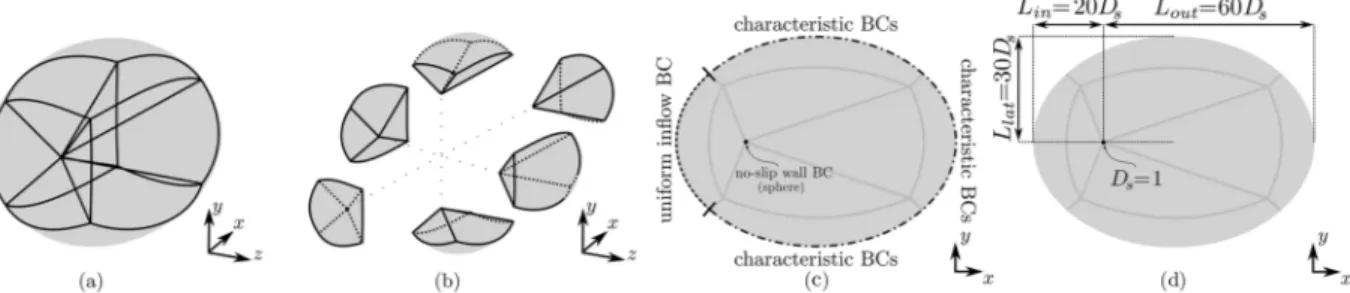
The numerical domain is composed of six blocks and its topol-ogy is displayed in Figs. 1(a) and 1(b). The grid resolution is (nx, ny, nz) = (281, 141, 141) for each block, considering a fine clustering of grid points in the vicinity of the sphere walls and in the wake region. To avoid spurious reflections, the grid is stretched near all lateral boundaries and outflow. Inflow, outflow, and lateral boundaries are set to beLin=20D∗s,Lout=60D∗s, andLlat=30D∗s, respectively. The center of the sphere is located at (x, y, z) = (0, 0, 0) and its non-dimensional diameter is unitary. The location of bound-ary conditions and the main characteristic scales are presented in
FIG. 1. Assembled (a) and exploded (b) six-block grid topology. Location of boundary conditions (c) and domain characteristic length scales (d) with respect to the sphere diameter.
quantities and sphere diameter spans fromRe = 500 to 1300, having evidence of the existence of both regular and Hopf bifurcations in this range.23The flow conditions are summarized inTable I. Grid resolution and domain size sensitivity studies for both base flow solutions and global stability results are presented in theAppendix, ensuring the suitability of the present numerical setup.
IV. RESULTS
As a first exploratory campaign, fully 3D unsteady nonlinear simulations have been carried out forRe = 600, 850, and 1000. A probe located just downstream of the sphere at (x, y, z) = (1.0, 0.0, 0.0) is used to record the streamwise velocity time histories for the three cases. Similarly to the work of Nagataet al.,23while the cases atRe = 600 and 850 are steady, an unsteady periodic behavior at St = 0.134 appears for the Re = 1000 case (further details about the unsteady spatio-temporal dynamics are given in Sec.IV C).
The sphere wakes of these three cases fundamentally differ not only temporally but also spatially: while the wake is axisymmetric for Re = 600, the planar-symmetry characterizes the wakes at Re = 850 and 1000. The zero-streamwise velocity iso-line (black solid line) is plotted over the contours of the density gradient for the two perpen-dicularx–z (first row) and x–y (second row) planes for the solutions atRe = 600 [(a)–(d)], Re = 850 [(b)–(e)], and Re = 1000 [(c)–(f)] inFig. 2. The projection of the 3D streamlines onto both planes is also represented (white solid lines). The unsteady solution at Re = 1000 has been time-averaged over five periods (eight samples per period) of the periodic behavior recorded by the streamwise velocity probe. As the selection of the plane where the axisymmetry is lost is equiprobable, for better clarity, the anti-symmetry plane of any solution presented throughout the whole paper has been rotated to match thex–y plane. The bow shock that forms in front of the sphere is rather Reynolds-insensitive and it is steady also for the Re = 1000 case. The separated region downstream of the body TABLE I. Inflow parameters.
Free-stream Mach number M∞= 1.2
Free-stream stagnation temperature Ti,∞∗ =287 K Free-stream stagnation pressure p∗i,∞=1.013 × 10⁵Pa
Reynolds number Re ∈ [500; 1300]
switches from an axisymmetry structure atRe = 600 to a planar-symmetric one atRe = 850 and 1000. In a time-averaged sense, the separated region forRe = 1000 is significantly reduced in length with respect to the steadyRe = 850 case. The streamlines upstream of the bow shock are all parallel to the flow direction and spiral axisym-metrically downstream of the sphere forRe = 600. For the Re = 850 and 1000 cases, the streamlines are instead spiraling asymmetrically in thex–y plane and cause the sphere wake to bend upwards. The sphere wake flow atM∞ = 1.2 for these three representative cases, therefore, changes both its temporal and spatial characteristics in this Reynolds number range: the wake is first steady and axisym-metric atRe = 600, then steady and planar-symmetric at Re = 850, and finally unsteady and planar-symmetric atRe = 1000. Similarly to what happens at incompressible6,8,10,11,13,14 and compressible high-subsonic21,22,24speeds, the sphere wake first loses its axisymmetry and then its steady state, indicating the existence of a regular and a Hopf bifurcation, respectively.
To determine and characterize these two bifurcations from a global stability point of view, an appropriate choice of the base flow solutions needs to be done. Considering the type of bifurcations that the fully 3D unsteady nonlinear calculations indicate, it is pos-sible to conclude that for increasing Reynolds numbers, (a) steady axisymmetric base flow solutions become unstable with respect to the regular bifurcation and (b) steady planar-symmetric base flow solutions become unstable with respect to the Hopf bifurcation. In Sec.IV A, different approaches are used to obtain the base flow solu-tions depending on the nature of the bifurcation to be investigated and their main features are described.
A. Baseflow solutions
Based on the flow features identified by the fully 3D unsteady nonlinear calculations, the two following different strategies for the calculation of the base flow solutions used in the global stability analyses are adopted:
(1) Base flow solutions for the regular bifurcation—steady forced symmetry: The objective is to identify the bifurcation that causes the loss of the wake axisymmetry. In this sense, axisymmetric (and steady) solutions represent the sta-ble/unstable base flows below/above the regular bifurcation critical Reynolds number (Reregcr ). Thus, a new set of steady axisymmetric base flow solutions is obtained by artificially
FIG. 2. Three-dimensional streamlines projected onto x–z [(a)–(c)] and x–y [(d)–(f)] planes superimposed to the density gradient contours for the Re = 600 [(a) and (d)], Re = 850 [(b) and (e)], and Re = 1000 [(c) and (f)] cases. The separated region is indicated by the solid black line.
forcing the flow symmetry taking into consideration only a quarter of sphere in the Reynolds number rangeRe = 500– 750. The numerical domain is therefore longitudinally sliced via two perpendicular cuts passing through the sphere cen-ter and applying symmetry boundary conditions to the newly formed lateral boundaries. Although this set of base flow solutions has been obtained on a quarter of domain, it is important to stress that the stability calculations presented in Sec.IV Bare fully 3D. Thus, once the steady solution in the quarter of domain has sufficiently converged, a 3D axisym-metric solution must be constructed by revolution.
(2) Base flow solutions for the Hopf bifurcation—steady fully 3D: The objective is to identify the bifurcation that causes the onset of the unsteadiness in the planar-symmetric solutions. In this regard, steady (and planar-symmetric) solutions rep-resent stable/unstable base flows below/above the Hopf bifur-cation critical Reynolds number (ReHopfcr ). For this reason, the implicit pseudo-unsteady approach36at CFL = 10 is used to artificially filter any possible unsteadiness and obtain the fully 3D steady base flow solutions in the Reynolds number range Re = 600–1000. Since the steady calculations are fully 3D and no axisymmetry is artificially imposed, these base flow solutions can be either steady axisymmetric or steady planar-symmetric. While only the steady planar-symmetric solutions are used for the characterization of the Hopf bifurcation, this set of calculations can also serve to nonlinearly identify the regular bifurcation critical Reynolds number and verify the corresponding linear calculations. The wake axi-symmetry is, in fact, broken betweenRe = 645 and 650, as it will be con-firmed by the global linear stability results presented in Sec.
IV B.
Figure 3and Table IIsummarize the Reynolds number evo-lution of the base flow separated region lengths for the two calcu-lation strategies described above. The separation lengths for some
selected Reynolds numbers obtained with unsteady fully 3D calcu-lations are also reported. When the wake is planar-symmetric, the separated region length is calculated by operating an average in the azimuthal direction. If an unsteadiness onsets, the separation length is also time-averaged over five periods (eight samples per period) of the periodic behavior recorded by a streamwise velocity probe in the wake region.
BelowRe = 650, the fully 3D approach predicts an axisymmetric solution, suggesting that the regular bifurcation threshold is around this Reynolds number value. Similarly to the incompressible coun-terpart (as shown in the inset ofFig. 3, where the incompressible results from Sansicaet al.24are added), the separation length cal-culated with the fully 3D approach above the regular bifurcation is
FIG. 3. Reynolds number evolution of the separation region length for the steady forced symmetry (solid line with full circle symbols), steady fully 3D (dashed line with empty circle symbols), and unsteady fully 3D (dashed-dotted line with empty diamond symbols) approaches. All separation lengths are obtained by averag-ing in the azimuthal direction. The separation lengths for the unsteady fully 3D calculations are also time-averaged. The inset plot shows the results for the incom-pressible sphere wake flow, taken from the work of Sansica et al.24The same line styles are used to indicate the different wake configurations of the incompressible solutions.
TABLE II. Separation region lengths and symmetry characteristics for the steady
forced symmetry, steady fully 3D, and unsteady fully 3D calculations. AS and PS stand for axisymmetric and planar-symmetric solutions, respectively.
Steady Steady Unsteady
Forced symmetry Fully 3D Fully 3D
Re Lsep Lsep Lsep
500 2.620 (AS) × ×
550 2.730 (AS) × ×
600 2.830 (AS) 2.830 (AS) 2.830 - (AS)
620 2.865 (AS) 2.865 (AS) × 640 2.896 (AS) 2.896 (AS) × 645 2.904 (AS) 2.904 (AS) × 650 2.910 (AS) 2.900 (PS) × 675 2.948 (AS) 2.812 (PS) × 700 2.983 (AS) 2.774 (PS) × 750 3.045 (AS) 2.743 (PS) × 800 × 2.752 (PS) 2.752 (PS) 850 × 2.779 (PS) 2.779 (PS) 875 × 2.797 (PS) 2.797 (PS) 900 × 2.815 (PS) 2.553 (PS) 950 × 2.858 (PS) 2.330 (PS) 1000 × 2.901 (PS) 2.220 (PS)
shorter (in an azimuthally averaged sense) than the forced axisym-metric solution at the same Reynolds number. Another similarity with the incompressible sphere wake is the fact that the separated region length initially decreases just above the regular bifurcation to then monotonically increase after reaching a minimum. Below Re = 875, the unsteady fully 3D calculations predict steady solutions and indicate that the Hopf bifurcation must be around this Reynolds number value. In agreement with the incompressible counterpart, the span and time-averaged separated region aboveRe = 875 are significantly shorter than the corresponding steady solutions. Although the incompressible and supersonic results are qualitatively showing the same trends, some quantitative differences exist. While the non-dimensional separation length (or equivalently the size of the separation with respect to the sphere diameter) is much larger in the supersonic regime, the rate of growth of the unstable base flow separation lengths with the Reynolds number around the bifurcation is higher for the incompressible case. Another important quantita-tive discrepancy regards the Reynolds number difference between
the two bifurcations, which is about four times larger for the super-sonic case. These differences again confirm the stabilizing effect of the Mach number on the onset of instabilities.
B. Regular bifurcation
The fully 3D axisymmetric base flows, artificially obtained by the revolution of the steady solutions calculated on a quarter of sphere, are used to investigate the regular bifurcation for the Reynolds numbersRe = 600, 620, 640, 645, 648, 649, 650, 675, and 700. Global stability analysis is performed on these base flows, and the growth rate Reynolds number evolution of the least temporally damped/most temporally amplified non-oscillatory mode is plotted inFig. 4(a). The shaded area for negative values of σ indicates tem-porally damped modes. The regular bifurcation threshold can be identified for a critical Reynolds number ofReregcr = 650. As con-firmed by the fully 3D base flow calculations presented in Sec.IV A
and in agreement with the work of Nagata et al.,23 this critical Reynolds number value defines the transition from a steady axisym-metric solution to a steady planar-symaxisym-metric one. Interestingly, the slope of the growth rate Reynolds evolution around the incompress-ible regular bifurcation is lower than the supersonic one (see Ref.24). The full eigenspectrum for theRe = 700 case is presented inFig. 4(b), where it is possible to see that only the non-oscillatory eigenvalue at (σ, St) = (0.024, 0.0) is temporally amplified. Although not shown here, the modes on the continuous branch are spatially localized in the far wake. Generally, while modes belowSt = 0.05 preserve axisymmetry, those at higher frequencies have anm = 1 azimuthal character and resemble the mode shape responsible for the Hopf bifurcation (shown later in Sec.IV C).
The corresponding eigenmode is represented inFig. 5by plot-ting the real part of the streamwise, vertical, and transverse eigen-velocities. To better appreciate the azimuthal character of the mode, the streamwise, vertical, and transversal eigenvelocities (ˆu, ˆv, and ˆw, respectively) have been transformed from the Cartesian to cylindri-cal coordinates to obtain the streamwise, radial, and azimuthal (ˆux, ˆur, and ˆuθ, respectively) ones. All eigenvelocities in the present paper
have been normalized with the maximum of the real part of the streamwise eigenvelocity. The mode is characterized by an azimuthal distribution corresponding to anm = 1 mode, and the perturba-tions in the streamwise eigenvelocity extend far downstream of the sphere body. Two “petal-like” structures appear due to the expan-sions generated on the sphere downstream of the bow shock. It must be emphasized that, except for the petal-like structures appearing on the sphere caused by high compressibility effects, the resemblance of the eigenmode with its incompressible counterpart is evident.
FIG. 4. Regular bifurcation global stabil-ity analysis: (a) Reynolds number evolu-tion of the growth rate of the least tempo-rally damped/most tempotempo-rally amplified non-oscillatory global mode; (b) eigen-spectrum in the St–σ plane for the Re = 700 case. The stable part of the plots has been shaded in light gray.
FIG. 5. Global mode at (σ, St) = (0.024, 0.0) for the Re = 700 case: 2D iso-lines in the x–z and x–y planes (first and second rows, respectively), 3D iso-surfaces (third row), and 2D projections of the iso-lines in the y–z planes at x = 1, 4, 8, 12, 16, 20 (fourth row) of the real part of the streamwise (first column), radial (second column), and azimuthal (third column) eigenvelocities for the levelsˆux= ±0.05, ˆur= ±0.05, and ˆuθ= ±0.05, respectively. The white and black iso-lines and iso-surfaces indicate the positive and negative perturbation eigenvelocities, respectively. The base flow density gradient contours (levels between 0.0 and 2.0) are added to the planar visualizations, with the zero-streamwise velocity iso-line indicated by the dashed black line.
C. Hopf bifurcation
Before describing the global stability results for the Hopf bifur-cation, nonlinear unsteady fully 3D simulations are performed at Re = 800, 850, 875, 900, 950, and 1000 to give a qualitative vali-dation against that of Nagataet al.23and provide a verification of the corresponding linear calculations. The nonlinear unsteady fully 3D calculations are restarted from the corresponding steady planar-symmetric fully 3D solution and let evolve in time. No forcing has been explicitly added to the simulation, and the unsteadiness slowly builds up from numerical noise. Similarly to the work of Nagata et al.,23 an unsteadiness only appears above Re = 875. The time
evolution of the streamwise velocity recorded by a probe in the sphere wake at (x, y, z) = (1.0, 0.0, 0.0) is reported inFig. 6(a)for the Re = 1000 case, showing a long linear transient between the (initial) steady solution and the nonlinearly saturated state. The linear tran-sient and part of the nonlinearly saturated state have been removed up tot ≈ 1400 (indicated by the dashed vertical gray line), and the corresponding power spectral density (PSD), calculated over about 85 periods of the dominant hairpin shedding frequency, is shown in
Fig. 6(b), indicating a limit cycle of self-sustained periodic oscilla-tions at a Strouhal number ofSt = 0.134. The velocity time history during the linear transient phase preceding the limit cycle evolves with a specific “nonlinear” growth rate, σNL. Despite the fact of being
FIG. 6. Unsteady nonlinear calculation at Re = 1000: (a) time evolution of the streamwise velocity in the sphere wake at (x, y, z) = (1.0, 0.0, 0.0) and (b) corresponding power spectral density. A zoom on the linear transient of the natural logarithm of the absolute value of the base flow subtracted streamwise velocity time evolution (c) shows the nonlinear growth rateσNL.
FIG. 7. Unsteady nonlinear calculation at Re = 1000: planar [(a) and (b)] and 3D (c) views of the iso-surfaces of the Q-criterion at a level of Q = 0.5. The instantaneous density gradient contours are also added (levels between 0.0 and 2.0).
calculated during the linear transient phase, the term “nonlinear” refers here to the type of calculation to avoid confusion with the “lin-ear” growth rate calculated by global stability analysis.Figure 6(c)
shows a zoom of the linear transient phase in the natural logarith-mic scale for the absolute value of the base flow subtracted stream-wise velocity time evolution. The calculated nonlinear growth rate is
σNL≈0.054. The spatial flow configuration is visualized by the pla-nar and 3D views of the Q-criterion iso-surfaces inFig. 7, where the instantaneous density gradient contours are also added to the planar views. The Q-criterion iso-surfaces are colored by the streamwise velocity (the light to dark colors correspond to the levels from −0.35 to 1.15). Despite the existence of an axisymmetric bow shock in front of the sphere, these visualizations show that the unsteady dynam-ics in the sphere wake is characterized by planar-symmetric hairpin vortex shedding. A first important remark must be made on the fact that a very similar behavior characterizes the unsteady incompress-ible sphere wake above the Hopf bifurcation threshold, both in terms of non-dimensional frequency value and spatial structures.
To describe the Hopf bifurcation and precisely identify the threshold value, global stability analysis is performed forRe = 850, 870, 873, 874, 875, 876, 880, 900, 950, and 1000 on the fully 3D steady planar-symmetric base flows presented in Sec.IV A. The growth rate Reynolds number evolution of the least temporally damped/most temporally amplified oscillatory mode is plotted inFig. 8(a), where the shaded area for negative values of σ indicates stable base flow cases. The Hopf bifurcation threshold is identified for a critical Reynolds number ofReHopfcr = 875, defining the transition from steady to unsteady wake dynamics. The full eigenspectrum for the Re = 1000 case is presented inFig. 8(b), showing that the oscillatory eigenvalue at (σ, St) = (0.054, 0.124) is temporally amplified. First
of all, it is useful to remark that the growth rate predicted by lin-ear stability analysis and the one calculated in the transient phase of the nonlinear unsteady calculations atRe = 1000 (σNL≈0.054, see Sec.IV C) are the same, verifying the correct functioning of the lin-ear solver with respect to its nonlinlin-ear counterpart. As already seen for other flow configurations or regimes,14,24,46 the linear stability analysis predicted frequency is instead slightly underestimated with respect to the nonlinear one. The real part of the eigenvelocities cor-responding to the (σ, St) = (0.054, 0.124) mode is visualized inFig. 9. Similarly to the regular bifurcation, the temporally amplified mode above the Hopf bifurcation in the supersonic regime spatially resem-bles its incompressible counterpart. The velocity perturbations are packed into planar-symmetric structures whose wavelength is about 3 ×Dsand extend in the wake far downstream of the sphere. The planar-symmetry of this mode is not broken, i.e., it has the same spatial symmetry of the base flow. A quantitative difference between this supersonic Mach number and the incompressible counterpart is that the slope of the growth rate Reynolds evolution around the crit-ical instability onset value is lower (see Ref.24), meaning that for the supersonic case, the planar-symmetric steady state is preserved over a larger range of Reynolds numbers. The appearance of the Hopf bifurcation with respect to the regular one is, in fact, retarded. This retardation can be confirmed by comparing the difference between the Hopf and regular critical Reynolds numbers, being about 60 in the incompressible regime and 225 atM∞=1.2.
In the region of temporally damped eigenmodes (σ < 0) pre-sented in Fig. 8(b), one mode at (σ, St) = (−0.021, 0.142) seems to be moving away from the continuous branch and get closer to the temporally amplified region (σ > 0). It, therefore, seems natu-ral to wonder what happens to this mode for a further increase of
FIG. 8. Hopf bifurcation global stability analysis: (a) Reynolds number evolution of the growth rate of the least tempo-rally damped/most tempotempo-rally amplified unsteady global mode; (b) eigenspec-trum in the St–σ plane for the Re = 1000 case. The stable part of the plots has been shaded in light gray.
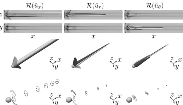
FIG. 9. Global mode at (σ, St) = (0.054, 0.124) for the Re = 1000 case: 2D iso-lines in the x–z and x–y planes (first and second rows, respectively), 3D iso-surfaces (third row), and 2D projections of the iso-lines in the y–z planes at x = 1, 4, 8, 12, 16, 20 (fourth row) of the real part of the streamwise (first column), radial (second column), and azimuthal (third column) eigenvelocities for the levelsˆux= ±0.20, ˆur= ±0.20, and ˆuθ= ±0.20, respectively. The white and black iso-lines and iso-surfaces indicate the positive and negative perturbation eigenvelocities, respectively. The base flow density gradient contours (levels between 0.0 and 2.0) are added to the planar visualizations with the zero-streamwise velocity iso-line indicated by the dashed black line.
the Reynolds number. The evolution and the characteristics of this mode are discussed in Sec.IV D.
D. Reflectional symmetry breaking bifurcation
The analysis of the Hopf bifurcation suggests the possibility to have multiple temporally amplified modes for increasing Reynolds number. While it is important to say that the bifurcation follow-ing the Hopf one should be analyzed by performfollow-ing the stability of the limit cycle with a Floquet analysis (i.e., on the unsteady peri-odic base flow), the objective of the present section is to spatially and temporally characterize the second bifurcation of the steady planar-symmetric base flow solutions. The observability of this instability in the nonlinear dynamics will be addressed in Sec.IV E. For this rea-son, and with the same principle adopted to obtain the base flow
solutions between Re = 600 and 1000 to study the Hopf bifurca-tion, steady fully 3D calculations are performed for only three other Reynolds numbers,Re = 1100, 1200, and 1300. The corresponding base flow solutions still present the same planar-symmetry found up toRe = 1000, and the azimuthally averaged base flow separation lengths areLsep= 2.992, 3.083, and 3.171 forRe = 1100, 1200, and 1300, respectively.
These steady planar-symmetric base flow solutions are used to perform global stability analysis. The mode mentioned in Sec.IV C, which atRe = 1000 was moving away from the continuous branch, becomes temporally amplified betweenRe = 1000 and 1100, indicat-ing the existence of a new bifurcation. In addition, a handful of other modes move away from the continuous branch and tend toward positive values of the growth rate. As well as the mode responsible for the Hopf bifurcation (named M1) and the second mode just found to become temporally amplified atRe = 1100 (named M2), the other
FIG. 10. (a) Eigenspectrum in the St– σ plane for the Re = 1300 case. (b) Reynolds number evolution of the growth rate of the modes leaving the continuous branch and indicated as M1–M6. The stable part of the plots has been shaded in light gray.
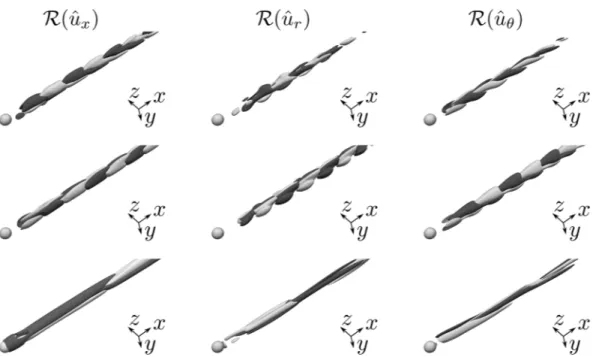
FIG. 11. Global stability modes at (first row—M1) (σ, St) = (0.137, 0.128), (second row—M2) (σ, St) = (0.062, 0.137), and (third row—M4) (σ, St) = (−0.016, 0.035) for the Re = 1300 case: 3D iso-surfaces of the real part of the streamwise (first column), radial (second column), and azimuthal (third column) eigenvelocities for the levelsˆux= ±0.20, ˆur= ±0.20, and ˆuθ= ±0.20, respectively. The white and black iso-lines and iso-surfaces indicate the positive and negative perturbation eigenvelocities, respectively.
modes moving away from the continuous branch are named M3, M4, M5, and M6 based on their vicinity to the temporally ampli-fied region of the spectrum and indicated inFig. 10(a), where the eigenspectrum for theRe = 1300 case is shown. The Reynolds num-ber evolution of modes M1–M6 is tracked by using dark gray full circle symbols and arrows in Fig. 10(a) but also explicitly plot-ted inFig. 10(b). Modes M3–M6 approach more or less rapidly
σ = 0, but all remain stable for this Reynolds range, at least up to
the highest Reynolds number investigated. While the identification of further bifurcations due to these modes is not intended, it is rel-evant to look at the corresponding eigenfunctions. Since mode M3 is just a longer wavelength version of M2 and modes M5 and M6 are practically identical to M1 and M2, respectively, only the M1,
M2, and M4 modes are plotted inFigs. 11and12. While mode M1 virtually presents no differences with respect to the mode respon-sible for the Hopf bifurcation reported inFig. 9except for being localized slightly closer to the sphere, it is interesting to see that the newly temporally amplified mode M2 corresponds to a 90○ rota-tion of mode M1 with respect to thex-axis. Following the defini-tion proposed by Fabre, Auguste, and Magnaudet,11who refer to the dominant mode that retains the base flow symmetry as “reflec-tional symmetry preserving” and to the sub-dominant rotated mode as “reflectional symmetry breaking,” the newly found bifurcation is named “reflectional symmetry breaking” bifurcation. Although at supersonic speeds, this reflectional symmetry breaking bifurcation confirms the intuition of Fabre, Auguste, and Magnaudet11and what
FIG. 12. Global stability modes at (first column—M1) (σ, St) = (0.137, 0.128), (second column—M2) (σ, St) = (0.062, 0.137), and (third column—M4) (σ, St) = (−0.016, 0.035) for the Re = 1300 case: 2D iso-lines projected onto (first row) the x–y planes and (second row) several y–z planes at x = 1, 4, 8, 12, 16, 20 of the real part of the streamwise eigenvelocities for the levelsˆux= ±0.20. The white and black iso-lines indicate the positive and negative perturbation eigenvelocities, respectively. The base flow density gradient contours (levels between 0.0 and 2.0) are added to the planar visualizations with the zero-streamwise velocity iso-line indicated by the dashed black line.
FIG. 13. Reynolds number evolution of the separation region length for the steady fully 3D (dashed line with empty circle symbols) and unsteady fully 3D (dashed-dotted line with empty diamond symbols). All separation lengths are obtained by averaging in the azimuthal direction. The separation lengths for the unsteady fully 3D calculations are also time-averaged.
found by Sansicaet al.24for incompressible cases, for which an anti-symmetric sub-dominant mode becomes temporally amplified if the Reynolds number is sufficiently large. Although M4 is just a longer wavelength version of M1, it was preferred to plot this mode rather than the less temporally damped M3 for comparisons that will be done in Sec.IV E. It should be noted that none of these modes breaks the planar-symmetry of the base flow. Finally, the reader should also keep in mind that M3 and M6 are also rotated of 90○, in the same way as for mode M2.
E. Observability of the reflectional symmetry breaking bifurcation in the nonlinear wake dynamics
The reflectional symmetry breaking bifurcation described in Sec. IV D was found for steady planar-symmetric base flow solutions. However, the bifurcation successive to the Hopf one should be instead sought by performing a limit cycle stability study
on the unsteady periodic base flow with a Floquet analysis (out of scope for the present work). The observability of the reflectional symmetry breaking bifurcation in the nonlinear wake dynamics is therefore addressed by performing nonlinear unsteady calculations at Re = 1100, 1200, and 1300. The nonlinear unsteady calcula-tions have been restarted from the corresponding steady planar-symmetric base flow solutions, in the same way done for the non-linear analysis shown in Sec.IV CforRe = 1000. As the flow features atRe = 1100 and 1200 are very similar to those at Re = 1300, the analysis will mainly focus on the comparisons of the latter with the Re = 1000 case.
At saturation, the nonlinear time-averaged solution is calcu-lated by collecting eight samples per period of the frequency at St = 0.148, over five periods of the lowest peak at St = 0.024. The time and azimuthally averaged separation lengths (dashed-dotted line with empty diamond symbols) are plotted in Fig. 13 with the azimuthally averaged separation lengths of the corresponding base flow solutions (dashed line with empty circle symbols). For increasing Reynolds number, the nonlinear time-averaged separa-tion length tends to reach a minimum, similarly to what found at incompressible regimes.14,24,47
The time evolution of the streamwise velocity recorded in the sphere wake at (x, y, z) = (1.0, 0.0, 0.0) is reported inFig. 14(a)
for theRe = 1300 case. The initial linear transient is removed up tot ≈ 350 [indicated by the vertical gray dashed line inFig. 14(a)], and the corresponding PSD distribution, calculated over about 70 periods of the dominant hairpin shedding frequency, is shown in
Fig. 14(b). It is possible to see that the spectrum is much richer with respect to the one at Re = 1000 (Fig. 6) and many peaks appear also at lower frequencies [St =O(10−2)]. The mid frequency energy peaks [St = O(10−1)] are in the same Strouhal number range of the linear dominant and reflectional symmetry breaking instabilities and represent possible candidates to be their nonlinear counterparts.
FIG. 14. Unsteady nonlinear calculation at Re = 1300: (a) time evolution of the streamwise velocity fluctuations in the sphere wake at (x, y, z) = (1.0, 0.0, 0.0) and (b) corresponding power spectral density.
FIG. 15. Unsteady nonlinear calcula-tion at Re = 1000 (first column) and Re = 1300 (second column): planar views of the iso-surfaces of the Q-criterion at a level of Q = 0.5. The instan-taneous density-gradient contours (lev-els between 0.0 and 2.0) are added to the planar visualizations.
TABLE III. Nonlinear interaction analysis for the Re = 1300 case. The peaks are numbered and indicated inFig. 14.
Peak no. 1 2 3 4 5 6 7 8 9 10 11 12 13
Strouhal 0.024 0.041 0.065 0.083 0.107 0.125 0.148 0.188 0.213 0.232 0.256 0.297 0.340
f0− 3f1 f1 f0− 2f1 2f1 f0− f1 3f1 f0 f0+f1 2f0+ 2f1 f0+ 2f1 2f0− f1 2f0 2f0+f1
The instantaneous Q-criterion iso-surfaces for theRe = 1000 (first column) andRe = 1300 (second column) cases are plotted in the planar views reported inFig. 15and colored by the streamwise velocity (the light to dark colors correspond to the levels from −0.35 to 1.15). No large differences can be discerned, except for a slightly shorter wavelength of the shed hairpin vortices for theRe = 1300 case, in agreement with a slightly higher shedding frequency (St = 0.134 for the Re = 1000 case vs St = 0.148 for the Re = 1300 case). It is also important to say that for the Reynolds number range considered, no wake modulation, oscillation, or helical motions were found like at lower Mach numbers.23
One last comment regards the Reynolds evolution of the problem nonlinearity. While from the spectrum in Fig. 6for the Re = 1000 case, it is easily recognizable the presence of the funda-mental frequency atSt = 0.134 and its first (St = 0.268) and second (St = 0.402) harmonics, for the Re = 1300 case, the analysis is rela-tively more complex. The latter is strongly nonlinear, and it is nec-essary to distinguish the fundamental frequencies, heref0andf1, and what results from nonlinear interactions, i.e., the harmonicsnf0 andmf1and quadratic or triadic interactions:nf0±mf1withn, m being the real positive integers. By takingf0= 0.148 (peak “P7” in
Fig. 14) andf1= 0.041 (peak “P2”), we can, for example, obtain 2f0 = 0.296 (peak “P12”),f0+f1= 0.189 (peak “P8”),f0−f1= 0.107 (peak “P5”), and so on. The nonlinear interactions for all peaks in
Fig. 14forPSD values above 10−4are summarized inTable III. By subtracting the mean value and normalizing the oscillation ampli-tude of the lift-coefficient time-histories, the phase plots [ ˆCL(t) vs ˙ˆCL(t)] reported inFig. 16reinforce the perception of different non-linear dynamics complexity atRe = 1000 and Re = 1300. The phase space passes from a limit cycle forming a single loop (Re = 1000) to a new limit cycle with three or four loops (Re = 1300). This indicates that the low frequency peak found atSt = 0.041 for the Re = 1300 case may be linked to the destabilization of the limit cycle atSt = 0.148.
F. Dynamic mode decomposition analysis
Since the Floquet analysis is out of scope for the present work, an alternative methodology to shed some light on the observ-ability of the reflectional symmetry breaking bifurcation can be given by a DMD analysis31 performed on the unsteady nonlinear calculations.
FIG. 16. Mean value subtracted and amplitude normalized lift-coefficient phase plots for the Re = 1000 (first row) and Re = 1300 (second row) cases. The darker color of the trajectory indicates the time advancement.
FIG. 17. DMD growth rates for the Re = 1000 (a) and Re = 1300 (b) cases represented by full black circles. The cor-responding PSDs are also reported as a solid gray line. The modes selected using the compressive sensing tech-nique are indicated by the dark dashed-line circles.
FIG. 18. DMD mode at St = 0.134 for the Re = 1000 case: 2D iso-lines in the x–z and y–z planes (first and second rows, respectively), 3D iso-surfaces (third row), and 2D projections of the iso-lines in the x–y planes at x = 1, 4, 8, 12, 16, 20 (fourth row) of the real part of the streamwise (first column), radial (second column), and azimuthal (third column) eigenvelocities for the levelsˆux= ±0.20, ˆur= ±0.20, and ˆuθ= ±0.20, respectively. The white and black iso-lines and iso-surfaces indicate the positive and negative perturbation eigenvelocities, respectively. The time-averaged density gradient contours (levels between 0.0 and 2.0) are added to the planar visualizations with the zero-streamwise velocity iso-line indicated by the dashed black line.
For theRe = 1000 and 1300 cases, 350 snapshots with a tem-poral interval of 1.057 are collected at saturation. The snapshots are 3D flow fields composed of density, velocities, and pressure for each domain cell and therefore very large. The conventional DMD approach31is limited by the large memory required. For this rea-son, low-dimensionalization is applied to the input dataset.48Eighty one proper orthogonal decomposition (POD) modes are obtained by incremental POD49and used for the dimensionality reduction. Total-least-squares DMD50was then applied to the low dimensional datasets. The dominant DMD modes are identified by means of the compressive sensing technique based on the greedy approach.51 Fur-ther details of the modal analysis framework can be found in the work of Ohmichi, Kobayashi, and Kanazaki,51where the “FBasis” modal analysis tool developed at the Japan Aerospace Exploration Agency (JAXA) is described in detail.
The DMD growth rates are reported in Fig. 17 for the Re = 1000 (a) and Re = 1300 (b) cases. The PSD distributions pre-sented inFigs. 6(b)and14(b)have been added (solid dashed gray line) to facilitate the correspondence of each peak with the DMD modes. For theRe = 1000 case, the compressive sensing technique identifies as dominant DMD modes those at frequencies (in order of dominance)St = 0.134, 0.268, and 0.402. These modes correspond to the three peaks found in the PSD distribution. The most domi-nant mode is the one atSt = 0.134, and the other two only represent its first and second higher harmonics, which will therefore not be discussed. The eigenvelocities corresponding to the dominant fun-damental DMD mode are reported inFig. 18. A strong link with
the nonlinear dynamics exists, and the footprint of the shed hair-pins seems clearer in the DMD eigenfunctions, as visible from the azimuthal eigenvelocity component. One of the main discrepancies between the global stability and the DMD modes consists of the dif-ferent development of the eigenwake in the streamwise direction. As shown inFig. 19, both eigenwakes have similar wavelengths and bend upwards following the deflection of the separated region (indi-cated by the dashed line). While the wake of the global stability mode is confined in a narrow region behind the sphere, the DMD mode diverges while moving downstream of the body. The distortion of the basic flow by nonlinear effects and larger diffusion is at the ori-gin of this spreading effect. The latter is taken into account in the
FIG. 19. Re = 1000 case: comparison between the streamwise eigenvelocities of the global stability (top) and DMD (bottom) modes. The base flow (top) and time-averaged (bottom) density gradient contours (levels between 0.0 and 2.0) are added to the planar visualizations with the zero-streamwise velocity iso-lines indicated by the dashed black line.
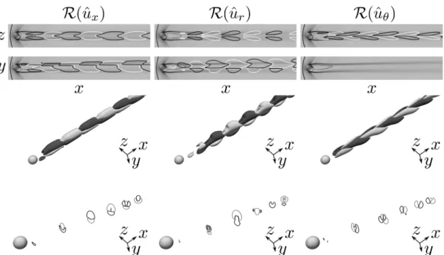
FIG. 20. DMD modes for the Re = 1300 case at (first row) St = 0.148, (second row) St = 0.041, (third row) St = 0.190, and (fourth row) St = 0.107: 3D iso-surfaces of the real part of the streamwise (first column), radial (second column), and azimuthal (third column) eigenvelocities for the levelsˆux= ±0.20, ˆur = ±0.20, and ˆuθ= ±0.20, respectively. The white and black iso-surfaces indicate the positive and negative perturbation eigenvelocities, respectively.
FIG. 21. DMD modes for the Re = 1300 case at (a) St = 0.148, (b) St = 0.041, (c) St = 0.190, and (d) St = 0.107: 2D iso-lines projected onto the y–z plane at x = 4 of the real part of the streamwise eigenvelocities for the levels ˆux = ±0.20. The white and black iso-lines indicate the positive and nega-tive perturbation eigenvelocities, respec-tively. The time-averaged density gradi-ent contours (levels between 0.0 and 2.0) are added in the background with the zero-streamwise velocity iso-line indicated by the dashed black line.
time-averaged flow, around which the DMD modes are calculated. Despite these differences, the similarities with the temporally ampli-fied global mode presented inFig. 9are evident. Both the global and the DMD modes are arranged spatially in packets of similar wave-length shape, have the same azimuthal character, and extend very far downstream of the body in the sphere wake region. To further high-light the similarities between the dominant global stability and DMD modes, two movies (“Re1000-GSA-Mode.mp4” and “Re1000-DMD-Mode.mp4” for the global stability and DMD modes, respectively) of the iso-surfaces of the eigenvelocities for the same levels presented in
Figs. 9and18(top: ˆux, middle: ˆur, and bottom: ˆuθ) during six periods
of their corresponding frequency are provided as thesupplementary material.
The compressive sensing technique for theRe = 1300 case indi-cates as most dominant modes those at (in order of dominance) St = 0.148, 0.041, 0.296, 0.190, and 0.107. While the St = 0.296 mode is just the first harmonic ofSt = 0.148, the eigenvelocities corre-sponding to the remaining four DMD modes are reported inFigs. 20
and 21. TheSt = 0.148 mode [first row inFigs. 20 and21(a)] is the same found as dominant in the DMD analysis at Re = 1000 and represents the nonlinear counterpart of the dominant linear global instability. TheSt = 0.041 [second row inFigs. 20and21(b)], St = 0.190 [third row inFigs. 20and21(c)], andSt = 0.107 [fourth row inFigs. 20and21(d)] DMD modes present some similarities with the dominant mode but at a higher level of spatial complexity due to nonlinear interactions. All the dominant modes have retained planar-symmetry, and no reflectional symmetry breaking ones are present. To make sure the reflectional symmetry breaking mode is not present among the sub-dominant modes, all DMD modes were carefully checked, but no evidence was found. It can there-fore be concluded that the global stability mode responsible for the reflectional symmetry breaking bifurcation is not observable in the nonlinear wake dynamics.
V. CONCLUSIONS
The increase of Mach number has a stabilizing effect on the sphere wake dynamics.21–25 At supersonic speeds, no evidence of the regular and Hopf bifurcations, respectively, responsible for the loss of axisymmetry and the appearance of unsteadiness in incom-pressible sphere wakes, was found in both nonlinear22,25and linear24 frameworks. The Reynolds number must be significantly increased in order for these unstable bifurcations to reappear.23
A global stability analysis is here carried out for sphere wakes at M∞ = 1.2 in the Reynolds number range Re ∈ [500; 1300]. Steady axisymmetric and steady planar-symmetric base flow solu-tions are selected to investigate the regular and Hopf bifurcasolu-tions, respectively. The steady axisymmetric base flows, obtained by forc-ing the axisymmetry on a quarter of sphere, are found to become unstable at a critical Reynolds number ofReregcr =650, identifying a steady planar-symmetric mode to be responsible for the occurrence of a regular bifurcation. The steady planar-symmetric base flows, instead, show the appearance of a Hopf bifurcation atReHopfcr =875, where an unsteady planar-symmetric eigenmode is the cause for the periodic hairpin vortex shedding in the sphere wake. Some dif-ferences intrinsic of the highly compressible flow conditions exist with respect to the incompressible counterparts. The supersonic
base flows are characterized by the formation of a bow shock in front of the sphere and the presence of expansions on the sphere body. The critical Reynolds numbers at M∞ = 1.2 move toward higher values, and the difference between the two critical thresholds is more than four times bigger than in the incompressible regime. However, remarkably similar features exist between incompressible and compressible (up to supersonic) configurations. The same types of unstable bifurcations persist, and the wake dynamics is anal-ogous in both spatial and temporal senses. This work, therefore, closely links the laminar sphere wake dynamics over a large range of flow velocities, from incompressible to (at least low) supersonic regimes.
At Re = 1000, the global stability analysis shows that a sub-dominant mode is approaching the temporally amplified region of the spectrum. For this reason, the global stability analysis performed on steady axisymmetric base flows is extended up to Re = 1300. The sub-dominant mode becomes temporally amplified between Re = 1000 and Re = 1100 and its spatial distribution corresponds to a 90○ rotation of the dominant mode, confirming some spec-ulations done on the sphere wake instabilities in the incompress-ible flow regime about the existence of a “reflectional symmetry breaking” bifurcation.11,24The latter was, however, found by global stability analysis performed around steady planar-symmetric base flow solutions, while to study the bifurcation successive to the Hopf one, a periodic base flow solution should instead be used for a Flo-quet analysis. FloFlo-quet analysis being out of scope for the present work, the observability of this reflectional symmetry breaking bifur-cation in the nonlinear wake dynamics is checked by carrying out unsteady nonlinear calculations in the rangeRe = 1000–1300. The wake spectral energy content interests a wide range of frequencies as the Reynolds number increases, and several PSD peaks, representing potential nonlinear counterparts of the linear instabilities, appear. For bothRe = 1000 and Re = 1300, DMD analysis indicates the dominant mode to be related to the nonlinear hairpin vortex shed-ding and its spatial distribution closely resembles the corresponshed-ding global stability mode responsible for the Hopf bifurcation. AtRe = 1300, many sub-dominant modes are also detected, but evidence of nonlinear reflectional symmetry breaking modes was not found. The wake dynamics seems rather to be governed by nonlinear inter-actions that suggest the low frequency unsteadiness to be related to the destabilization of the hairpin vortex shedding limit cycle.
The absence of rotated DMD modes shows the need to perform global stability Floquet analysis on periodic base flows to charac-terize physical bifurcations successive to the Hopf one. Evidence of wake modulations and wake helical motions superimposed to the hairpin vortex shedding exists at lower speeds,23suggesting the possibility to determine subsequent bifurcations and offering future investigation opportunities. It is in the authors’ opinions that due to the stabilizing effect of the Mach number (as seen in Ref.23), the same mechanisms presented here might be preserved at higher speeds, most likely just accompanied by a shift of the critical Reynolds numbers toward higher values. Only for much higher Mach numbers in the hypersonic range, for which the bow-shock forming in front of the body will “wrap” closely around the sphere, new physics might appear. Finally, another regime of interest could be the transonic one, for which shocks will form on the sphere sur-face or on the sphere wake and may be generating some buffet-like phenomenon.
SUPPLEMENTARY MATERIAL
See the supplementary material for the temporal anima-tions of the global stability (“Re1000-GSA-Mode.mp4”) and DMD (“Re1000-DMD-Mode.mp4”) modes atRe = 1000 during six periods of their corresponding frequency. The iso-surfaces of the streamwise (top plot), radial (middle plot), and azimuthal (bottom plot) eigen-velocities for the levels ˆux = ±0.20, ˆur = ±0.20, and ˆuθ = ±0.20, respectively. The white and black iso-surfaces indicate the positive and negative perturbation eigenvelocities, respectively.
APPENDIX: SOLVER VALIDATION AND SENSITIVITY STUDIES
1. Validation
The same numerical setup and grid described in Sec.IIIare used for the validation of the nonlinear solver. The results obtained with the present solver are compared over a range of different speeds, from the incompressible regime to the supersonic one. For the incompressible regime, the experimental results of Taneda52 and the numerical ones by Tomboulides, Orszag, and Karniadakis,7 Magnaudet, Rivero, and Fabre,53 and Johnson and Patel54 in the Reynolds number range betweenRe = 25 and 200 are selected. To approximate the incompressible flow conditions with the present compressible solver, the Mach number has been set toM∞= 0.1. In agreement with the literature, for each Reynolds number consid-ered (Re = 25, 50, 100, 150, and 200), the solutions consist of steady and axisymmetric wakes. The length of the separated region for each Reynolds number is plotted inFig. 22, where the benchmark solu-tions are also added. The agreement with the literature is remarkable and the present results almost coincide with those of Tomboulides, Orszag, and Karniadakis.7To verify the effects of compressibility up to supersonic speeds, the works of Johnson and Patel54and Nagata et al.22(the values have been digitalized from the paper) are used, andTable IVsummarizes the validation test results by listing the separation lengths for different Mach numbers atRe = 150. In agree-ment with the benchmark solutions, the wakes are all steady and axisymmetric. An excellent comparison is obtained against Johnson and Patel54atM
∞= 0.3, for which the relative percentage error is below 2.5%. Considering that the work by Nagataet al.22is the only present in the literature for this range of Mach and Reynolds num-bers, for theM∞= 0.8 and 1.2 cases, the relative percentage error is
FIG. 22. Validation for incompressible sphere wake test cases.
TABLE IV. Validation for compressible (up to supersonic) sphere wake separation
lengths. The results are compared against those of Nagata et al.22(NNT&F) and
Johnson and Patel54(J and P).
Mach Reynolds Present NNT&F Δerr (%) J and P Δerr (%)
0.30 150 1.25 1.14 9.65 1.22 2.46
0.80 150 1.78 1.74 2.30 × ×
1.20 150 0.90 0.95 5.26 × ×
around 5% or below. A general satisfactory agreement is achieved, and the correct functioning of the nonlinear solver is confirmed. 2. Grid resolution and domain sensitivity studies
The sensitivity of both base flow solutions and global stabil-ity analysis to grid refinement and domain size is here presented. The reader should note that the six-block elliptical domain topol-ogy is maintained for all cases. The domain and grid resolution used to produce the results presented in Sec.IVare indicated as G1-D1. For the grid refinement study, the domain size is kept fixed and a coarser grid with (nx,ny,nz) = (225, 113, 113) per block (named G0-D1) and a finer grid with (nx, ny, nz) = (337, 169, 169) per block (named G2-D1) are considered. For the domain size sensi-tivity study, a smaller domain with (Lin,Lout,Llat) = (10, 30, 15) (named G1-D0) and a larger domain with (Lin,Lout,Llat) = (40, 120, 60) (named G1-D2) are used. The grid distribution is kept fixed, and elliptical layers of grid points are simply removed or added to account for a smaller or larger domain. For this reason, the grid res-olution per block only changes only in the radial direction and is (nx,ny,nz) = (225, 141, 141) and (nx,ny,nz) = (316, 141, 141) for the G1-D0 and G1-D2 cases, respectively. These details of the grid resolution and domain size are summarized inTable V. To evaluate the effect of grid refinement and domain size, the separation length and the least temporally damped/most temporally amplified eigen-value are chosen as sensitivity indicators for the base flow solution and global stability analysis, respectively. Two Reynolds numbers are selected for each bifurcation in order to consider a stable and an unstable case:Re = 600 and Re = 650 for the regular and Re = 850 and Re = 900 for the Hopf bifurcation.Table VIreports the values of the sensitivity indicators for the examined cases along with the relative percentage error with respect to the values of the G1-D1 case. For all cases, the base flow separation length sensitivity is below 2.5% and the numerical grid/domain G1D1 used as reference through-out the paper can therefore be considered suitable for the base flow
TABLE V. Sensitivity studies on grid resolution and domain size. Details of the
numerical setup.
Case nx×ny×nz Lin×Lout×Llat
G1-D1 281 × 141 × 141 20 × 60 × 30
G0-D1 225 × 113 × 113 20 × 60 × 30
G2-D1 337 × 169 × 169 20 × 60 × 30
G1-D0 225 × 141 × 141 10 × 30 × 15
![FIG. 2. Three-dimensional streamlines projected onto x–z [(a)–(c)] and x–y [(d)–(f)] planes superimposed to the density gradient contours for the Re = 600 [(a) and (d)], Re](https://thumb-eu.123doks.com/thumbv2/123doknet/7430959.219807/6.891.109.790.128.390/dimensional-streamlines-projected-planes-superimposed-density-gradient-contours.webp)

![FIG. 7. Unsteady nonlinear calculation at Re = 1000: planar [(a) and (b)] and 3D (c) views of the iso-surfaces of the Q-criterion at a level of Q = 0.5](https://thumb-eu.123doks.com/thumbv2/123doknet/7430959.219807/9.891.67.556.125.328/unsteady-nonlinear-calculation-planar-views-surfaces-criterion-level.webp)