ANALYSES SPATIALES DE LA BIODIVERSITÉ
BENTHIQUE DU GOLFE SAN JORGE, ARGENTINE
SPATIAL ANALYSES OF BENTHIC BIODIVERSITY IN SAN JORGE
GULF, ARGENTINA
Mémoire présentée
dans le cadre du programme de maîtrise en océanographie en vue de l’obtention du grade de maître ès sciences
PAR
© JULIETA KAMINSKY
Composition du jury :
Gesche Winkler, Présidente du jury, ISMER Université du Québec à Rimouski Philippe Archambault, Directeur de recherche, Université Laval
Martín Varisco, Codirecteur de recherche, CIT Golfo San Jorge CONICET UNPSJB Ricardo Sahade, Codirecteur de recherche, IDEA CONICET UNC
Julio Vinuesa, Examinateur externe, CIT Golfo San Jorge CONICET UNPSJB
UNIVERSITÉ DU QUÉBEC À RIMOUSKI Service de la bibliothèque
Avertissement
La diffusion de ce mémoire ou de cette thèse se fait dans le respect des droits de son auteur, qui a signé le formulaire « Autorisation de reproduire et de diffuser un rapport, un
mémoire ou une thèse ». En signant ce formulaire, l’auteur concède à l’Université du
Québec à Rimouski une licence non exclusive d’utilisation et de publication de la totalité ou d’une partie importante de son travail de recherche pour des fins pédagogiques et non commerciales. Plus précisément, l’auteur autorise l’Université du Québec à Rimouski à reproduire, diffuser, prêter, distribuer ou vendre des copies de son travail de recherche à des fins non commerciales sur quelque support que ce soit, y compris l’Internet. Cette licence et cette autorisation n’entraînent pas une renonciation de la part de l’auteur à ses droits moraux ni à ses droits de propriété intellectuelle. Sauf entente contraire, l’auteur conserve la liberté de diffuser et de commercialiser ou non ce travail dont il possède un exemplaire.
In the end we will conserve only what we love, we will love only what we understand, and we will understand only what we are taught
Baba Dioum
La meilleure façon de réaliser ses rêves, c’est de se réveiller! Autrement dit, pour faire partie de la solution, il faut passer à l’action
Phil Jackson
Ella, la mar, estaba más allá de los altos médanos, esperando. Cuando el niño y su padre alcanzaron por fin aquellas cumbres de arena, después de mucho caminar, la mar estalló ante sus ojos. Y fue tanta la inmensidad de la mar, y tanto su fulgor, que el niño quedó mudo de hermosura. Y cuando por fin consiguió hablar, temblando, tartamudeando, pidió a su padre: —¡Ayúdame a mirar!
REMERCIEMENTS
Ici à Rimouski, j’ai connu l’hiver. J’ai connu une latitude où en été le Soleil ne veut pas partir, mais pendant l’hiver il se cache la plupart de la journée. J’ai vu un fleuve devenir gèle et des arbres se peinturer avec deux mil couleurs. J’ai commencé une maîtrise en Océanographie, dans un autre pays, dans une autre langue, dans une autre culture. J’ai tombé en amoureuse dans la forêt. J’ai appris à continuer apprendre, mais cette fois dans une autre matrix socio-culturelle. Surtout, j’ai rencontré des expériences académiques et scientifiques différentes, enrichissantes, pour toute ma vie. Je garde avec moi une panoplie des réflexions, des amis et des paysages, inoubliables. Merci pour ce voyage.
Tout d’abord, j’aimerais remercier le Programme BEC.AR (Argentina) pour m’avoir offert la bourse de maîtrise qui m’a permis de poursuivre cette merveilleuse expérience au Québec.
Je voudrais remercier l’ISMER-UQAR de m’avoir accepté pour poursuivre mes études de maîtrise en océanographie.
Merci beaucoup à Philippe Archambault de m’avoir accepté comme étudiante dans le Laboratoire benthique. Également, je voudrais remercier Martín Varisco et Ricardo Sahade d’avoir accepté la codirection de mon projet de maîtrise.
Merci beaucoup au Comité du jury pour vos commentaires et modifications suggérées qui ont enrichies mon mémoire.
x
Je voudrais remercier mes professeurs d’Océanographie générale et d’Océanographie expérimentale de m’avoir fourni un ensemble de concepts et d’outils pour aborder ma maîtrise.
Je voudrais remercier l’INIDEP, et particulièrement Mónica Fernández, de m’avoir offert un ensemble de données qui a permis de développer le présent projet. Également, je voudrais remercier Agustina Ferrando pour les données de polychètes, Marta Commendatore pour les données de sédiments et Gabriela Williams pour les données de bathymétrie.
Merci infiniment à Alain Caron pour m’avoir aidé à réfléchir dans les différentes étapes des analyses et de me donner une boîte d’outils statistiques. Merci de votre patience dans chaque rencontre où je suis arrivée avec ma feuille des questions.
J’aimerais remercier énormément Nathalie Landreville du CAR-UQAR pour son aide extraordinaire dans l’édition de mes présentations en français.
J’aimerais remercier Gustavo Ferreyra et Irene Schloss pour m’avoir accompagné dans chaque étape de la maîtrise, pour m’avoir orienté et m’avoir encouragé avec esprit et cœur.
Merci beaucoup au Laboratoire benthique pour l’aide dans différents moments de ma maîtrise. Je voudrais remercier spécialement Jésica Goldsmith, Cindy Grant, Gonzalo Bravo, Heike Link, Charlotte Moritz, Blandine Gaillard et Mylène Dufour de vos apports.
Merci beaucoup Pierre-Arnaud Desiage et Noela Sánchez-Carnero pour votre aide dans différents moments de mes analyses.
Je voudrais remercier Martine Belzile, Nancy Lavergne et Brigitte Dubé pour leur collaboration dans chaque étape. Merci à Marcel David pour m’avoir aidé dans mes voyages à la bibliothèque de l’UQAR.
De plus, j’aimerais remercier toutes les personnes avec qui j’ai partagé des expériences au Québec. Merci avec tout mon cœur aux filles argentines Maité, Xime, Elo et Ari pour partager ce voyage extraordinaire ensemble. Je vous admire énormément. Merci à toute la communauté argentine de Rimouski. Vous êtes merveilleux. Merci à Jesi, Nacho et Licho pour chaque mate et sourire partagés. Merci à María et Santiago pour votre belle amitié épicée. Merci à l’équipe de volley les étrangers pour jouer ensemble.
Merci à mes oncles Arlène et James pour m’avoir ouvert les portes à votre monde génial, pour m’avoir accompagné et nourri l’âme et l’esprit. Vous êtes inoubliables.
Merci à mon ami Marwen pour les réflexions collectives sur nos cultures, nos familles et nos vies. Je t’admire beaucoup. Merci à mes colocs pour la construction d’un
Bercail à Rimouski. Merci aux Bombones, et spécialement à Louis Poulain, à Sara Dignard
et à Tom Jacques, pour m’avoir fait rire, lire, écouter vraiment beaucoup. Merci Geneviève pour ton amitié, toujours pleine de réflexions et de mots tellement enrichissants.
Merci beaucoup à mes parents Mirta et Goyo, à mon frère Javier, à ma grand-mère Olga et aux amis en Argentine pour m’envoyer les plus belles énergies.
Merci à David, à ta magique famille, à notre petit Paprika et aux plantes pour l’amour.
AVANT-PROPOS
Le présent projet de recherche fait partie du programme PROMESse-MARES, développé par des institutions de l’Argentine et du Québec. Ce programme vise à décrire l’état présent de l’écosystème du golfe San Jorge (Argentine). Dans ce cadre, j’ai obtenu une bourse du programme BEC.AR (Argentine) pour poursuivre des études de maîtrise en océanographie à l’ISMER-UQAR. Pour la présentation écrite de mon devis de recherche, le Comité d’évaluation de l’ISMER m’a donnée une mention d’excellence. Je voudrais également souligner l’aide financière que j’ai reçu du Service aux Étudiantes de l’UQAR pour participer dans la mission océanographique du programme Pampa Azul au golfe San Jorge. Cette mission a été menée à bord du navire de recherche Puerto Deseado pendant le mois de novembre 2016. Cette expérience m’a permis de connaître mon site d’étude, faire des échanges avec des scientifiques qui travaille dans le même environnement et améliorer l’interprétation de mes résultats de maîtrise.
Durant la période de 2 ans, ce projet a été présenté dans les événements scientifiques suivants :
✓ Kaminsky J, Varisco M, Sahade R, Archambault P. Spatial analyses of
benthic biodiversity in the San Jorge Gulf. Présentation des résultats de
maîtrise. Mars 2017, Workshop PROMESse, Rimouski, Québec
✓ Kaminsky J, Varisco M, Sahade R, Archambault P. Functional benthic
ecology in an Argentinean Patagonian gulf: what is where? Affiche.
Novembre 2016, Assemblée Générale Annuelle Québec Océan, Rimouski, Québec
xiv
✓ Bravo G, Flores Melo X, Giménez E, Kaminsky J, Klotz P, Nocera A, Latorre M. Naviguons dans le Golfe San Jorge, Patagonie Argentine. Stand avec de l’information audiovisuel. Mars 2016, La nature dans tous ses états, UQAR, Rimouski, Québec
✓ Kaminsky J, Archambault P, Varisco M, Sahade R. Analyse spatiale de la
biodiversité benthique dans le golfe San Jorge, Argentine. Affiche. Novembre
2015, Assemblée Générale Annuelle Québec Océan, Québec, Québec
Les principaux résultats de recherche seront publiés à partir d’un thème spécial dans le journal scientifique Oceanography avec l’ensemble des résultats du PROMESse.
RÉSUMÉ
La distribution de la biodiversité benthique est liée à la complexité des habitats. Dans un contexte d’augmentation des pressions anthropiques, il est nécessaire de développer des modèles de biodiversité selon la distribution des habitats afin d'améliorer la gestion et la conservation des écosystèmes marins et côtiers. Le golfe San Jorge (45° - 47° S, Argentine) fait partie du Patagonian Shelf Large Marine Ecosystem, l'un des écosystèmes les plus productifs de l'hémisphère sud. L'objectif de cette étude était de caractériser la distribution spatiale de la biodiversité benthique du golfe de San Jorge (SJG). Nous avons décrit les caractéristiques de l'environnement benthique. Ensuite, nous avons exploré la présence des assemblages taxonomiques et fonctionnels pour l’épifaune et l'endofaune. Ensuite, nous avons évalué la relation entre l'environnement benthique et la distribution des assemblages pour estimer la probabilité de présence des assemblages. Nos hypothèses étaient que la distribution des assemblages est associée à la profondeur, à la granulométrie et à la matière organique, et que les assemblages les plus divers sont dans les zones à forte matière organique. Les données des missions R/V Oca Balda (2000) et R/V Coriolis (2014) ont été utilisées. Nos résultats montrent la présence des assemblages d’épifaune taxonomique et fonctionnels. La région centrale avec concentrations de matière organique plus élevées était caractérisée par d’opportunistes rampant et déposivores de subsurface creuseur. Dans le nord, près de l’embouchure et dans les côtes l’assemblage d’épifaune est composé par déposivores de subsurface, suspensivores sessile ou creuseur. Cet assemblage a été corrélé avec basses concentrations d’oxygène et de matière organique. Au contraire, l’épifaune est composée par prédateurs nageur, prédateurs rampant, opportunistes rampant et suspensivores sessile près de Cape Tres Puntas. Dans le cas de l'endofaune, aucun modèle spatial n'a été identifié, probablement en raison de l'effort d'échantillonnage. Les cartes avec les habitats préférentiels permettent de prédire la distribution de la biodiversité benthique dans le SJG, en particulier selon la disponibilité d’oxygène dans l’eau de fond et les concentrations de la matière organique de sédiments.
Mots clés : environnement benthique, assemblages, diversité fonctionnelle, modèle de
ABSTRACT
Benthic biodiversity distribution is closely related to habitat complexity. In the context of increasing anthropogenic pressures, it is necessary to develop biodiversity models considering habitat distribution to improve management and conservation of marine and coastal ecosystems. San Jorge Gulf (45° - 47° S, Argentina) is part of the Patagonian
Shelf Large Marine Ecosystem, one of the most productive ecosystems of the Southern
Hemisphere. The general objective of this study was to characterize the spatial distribution of benthic biodiversity of the San Jorge Gulf (SJG). First, we described the physic-chemical characteristics of the benthic environment. Then, we explored taxonomic and functional assemblages for epifauna and infauna organisms. Afterwards, we evaluated the relationship between benthic environment and assemblages’ distribution to estimate habitat suitability for assemblages. We hypothesized that the distribution of benthic assemblages is associated with depth, sediment size and concentration of sediment organic matter as environmental factors, and that the most diverse assemblages are present in areas with higher concentrations of organic matter. Data from R/V Oca Balda (2000) and R/V Coriolis (2014) oceanographic missions in SJG were used. Our results show the presence of epifauna taxonomic and functional assemblages. The central area of SJG with high organic matter is characterised by opportunist crawlers and deposit subsurface burrowers. In the north, close to the mouth and along the southern coastal area (Mazarredo), the epifauna assemblage was mainly composed by deposit subsurface feeders, filter burrowers and sessile feeders. This assemblage was correlated with low oxygen availability and low organic matter concentrations. On the contrary, assemblages close to Cape Tres Puntas were characterised by predator swimmers, predator crawlers, opportunist crawlers and filter sessile feeders. In the case of infauna, no spatial patterns were identified, probably related with the sampling effort. Habitat suitability maps might enable to predict benthic biodiversity distribution in the SJG, particularly considering oxygen availability in bottom water and organic matter in sediments.
Keywords: benthic environment, assemblages, functional diversity, biodiversity
TABLE DES MATIÈRES
REMERCIEMENTS ... ix
AVANT-PROPOS ... xiii
RÉSUMÉ ... xv
ABSTRACT ... xvii
TABLE DES MATIÈRES ... xix
LISTE DES TABLEAUX ... xxiii
LISTE DES FIGURES ... xxv
LISTE DES ABRÉVIATIONS, DES SIGLES ET DES ACRONYMES ... xxvii
INTRODUCTION GÉNÉRALE ... 1
PREDIRE LA DISTRIBUTION DE LA BIODIVERSITE BENTHIQUE ... 1
LA DIVERSITE FONCTIONNELLE DANS LES ASSEMBLAGES BENTHIQUES ... 3
LE GOLFE SAN JORGE ... 5
OBJECTIFS ET HYPOTHÈSES ... 6
CHAPITRE 1 ANALYSES SPATIALES DE LA BIODIVERSITÉ BENTHIQUE DU GOLFE SAN JORGE, ARGENTINE ... 8
1.1CONTEXTE DU PROJET ... 8
1.2SPATIAL ANALYSES OF BENTHIC BIODIVERSITY IN SAN JORGE GULF,ARGENTINE ... 9
1.3INTRODUCTION ... 9
1.4MATERIALS AND METHODS ... 13
xx
1.4.2 Data acquisition ... 15
1.4.3 Benthic environment ... 16
Spatial distribution of environmental variables ... 16
Correlation between environmental variables ... 16
1.4.3 Benthic diversity ... 17
Taxonomic diversity ... 17
Functional diversity ... 18
Regression model for local diversity ... 19
1.4.4 Relation between benthic environment and benthic diversity ... 20
1.4.5 Biodiversity distribution model for the San Jorge Gulf ... 20
1.5RESULTS ... 21
1.5.1 Benthic environment ... 21
Spatial distribution of environmental variables ... 21
Correlation between environmental variables ... 24
1.5.2 Benthic diversity and relations with benthic environment ... 27
Taxonomic epifauna diversity ... 27
Functional epifauna diversity ... 34
Taxonomic infauna diversity ... 41
Functional infauna diversity ... 43
Regression model for local diversity ... 45
1.6DISCUSSION ... 46
Description of benthic environment ... 46
Benthic assemblages description ... 47
Biodiversity distribution model for the San Jorge Gulf ... 50
Relation between species richness and functional groups richness ... 52
1.7CONCLUSION ... 53
Contributions de l’étude ... 56
Limitations de l’étude ... 56
Perspectives ... 57
ANNEXES ... 61
LISTE DES TABLEAUX
Table 1: List of functional groups and traits used for functional classification of taxa…… 19 Table 2 : Results from PCA considering INIDEP environmental data……… 25 Table 3 : Results from PCA considering MARES environmental data... 27 Table 4 : Taxonomic diversity indices for epifauna data by assemblage. The five dominant taxa in terms of total abundance of individuals by assemblage are presented………. 30 Table 5 : DistLM of epifauna taxonomic assemblages against environmental variables (Best-fit model with 9999 permutations, AICc = 208.1, R2 = 0.269)………. 31 Table 6 : Results for the second set of GLMs predicting the presence of taxonomic assemblages……….. 32 Table 7 : Functional diversity indices for epifauna data by assemblage. The five dominant functional groups in terms of total abundance of individuals by assemblage are presented………... 37 Table 8 : DistLM of functional epifauna assemblages against environmental variables (Best-fit model with 9999 permutations, AICc = 205.3, R2 = 0.305)………... 38 Table 9 : Results for the second set of GLMs predicting the presence of functional assemblages………... 39 Table 10 : DistLM of taxonomic infauna against environmental variables (Best-fit model with 9999 permutations and minimum two variables, AICc = 108.7, R2 = 0.250)……….. 42 Table 11 : DistLM of functional infauna assemblages against environmental variables (Best-fit model with 9999 permutations, AICc = 108.14, R2 = 0.27)………... 44
LISTE DES FIGURES
Figure 1 : Study site with sampling stations (bathymetry adapted from Carta H-365, Servicio de Hidrografía Naval, Argentina)………... 14 Figure 2 : Spatial distribution of sediment variables: gran size, total organic matter (TOM), total organic carbon (TOC) and total nitrogen (TN). Bathymetry is indicated by isolines...22 Figure 3 : Spatial distribution of bottom water variables: temperature, salinity, oxygen availability and chlorophyll a. Bathymetry is indicated by isolines………. 23 Figure 4 : Principal component analyses plots with the first two axes for INIDEP data. Stations (objects) and environmental variables (descriptors) are represented. Vectors indicate the direction and strength of environmental variables……….24 Figure 5 : Principal component analyses plots with the first two axes for MARES data. Stations (objects) and environmental variables (descriptors) are represented. Vectors indicate the direction and strength of environmental variables……….26 Figure 6 : Taxonomic cluster based on Bray-Curtis Similarity matrix using epifauna taxonomic abundance by station. The taxonomic epifauna assemblages are represented with different colors……….. 28 Figure 7 : Location of epifauna taxonomic assemblages in the SJG……… 29 Figure 8 : Distance-based redundancy analysis (dbRDA) plot of the DistLM based on the environmental variables best-fitted to the variation in epifauna taxonomic assemblages. Vectors indicate direction of the environmental variable in the ordination plot…………... 31 Figure 9 : Habitat suitability maps representing the probability of presence for taxonomic epifauna assemblages’ c and d in the SJG……… 33 Figure 10 : Functional cluster based on Bray-Curtis Similarity matrix using epifauna functional groups abundance by station. The functional epifauna assemblages are represented with different colors………... 34
xxvi
Figure 11 : Location of epifauna functional assemblages in the SJG………... 36 Figure 12 : Distance-based redundancy analysis (dbRDA) plot of the DistLM based on the best environmental variables fitted to the variation in epifauna functional assemblages. Vectors indicate direction of the environmental variable in the ordination plot…………... 38 Figure 13 : Habitat suitability maps representing the presence for epifauna functional assemblages’ c and d in the SJG………... 40 Figure 14 : Taxonomic cluster based on Bray-Curtis Similarity matrix using infauna taxonomic abundances by station. No assemblages were identified………. 41 Figure 15 : Distance-based redundancy analysis (dbRDA) plot of the DistLM based on the best environmental variables fitted to the variation in infauna taxonomic stations. Vectors indicate direction of the environmental variable in the ordination plot……… 42 Figure 16 : Functional cluster based on Bray-Curtis Similarity matrix using infauna functional groups abundances by station. No assemblages were identified………. 43 Figure 17 : Distance-based redundancy analysis (dbRDA) plot of the DistLM based on the best environmental variables fitted to the variation in functional infauna assemblages. Vectors indicate direction of the environmental variable in the ordination plot………... 44 Figure 18 : Linear regression model between local taxonomic and functional richness….. 45
LISTE DES ABRÉVIATIONS, DES SIGLES ET DES ACRONYMES
PROMESse Programa Multidisciplinario para el Estudio del ecosistema y la geología
marina del golfo San Jorge y las costas de las provincias de Chubut y Santa Cruz.
MARES Marine ecosystem health of the San Jorge Gulf: Present status and
Resilience capacity.
INIDEP Instituto Nacional de Investigación y Desarrollo Pesquero (Argentina). SJG San Jorge Gulf.
TOM Total organic matter. TOC Total organic carbon. TN Total nitrogen.
INTRODUCTION GÉNÉRALE
PRÉDIRE LA DISTRIBUTION DE LA BIODIVERSITÉ BENTHIQUE
La distribution de la biodiversité benthique est fortement liée à la complexité des habitats des écosystèmes côtiers et marins (Brown et al. 2011, Kovalenko et al. 2012, Moritz et al. 2013, Carvalho et al. 2017). Les habitats benthiques peuvent être décrits comme des régions de fonds marins qui sont géo-statistiquement différentes de leur environnement en termes de caractéristiques physiques, chimiques et biologiques, en considérant des échelles d’observations spatiales et temporelles précises (Lecours et al. 2015). Une panoplie de facteurs environnementaux qui varient sur les plans spatiaux et temporels déterminent la présence d’une grande hétérogénéité d’habitats dans les environnements benthiques. Parmi ces facteurs, ont été principalement décrites des variations dans la topographie (Archambault et Bourget 1996, Archambault et al. 1999), la présence des structures physiques (Carvalho et al. 2017) et la taille de sédiments (Gray et Elliot 2009). La circulation des masses d’eau détermine fortement les caractéristiques physico-chimiques, comme la température, la salinité et la présence de nutriments. La dynamique dans la colonne d’eau peut conditionner le couplage pélagique-benthique et la disponibilité et la qualité des apports de matière organique qui arrivent au fond (Wassmann 1997). De plus, la topographie, les structures physiques et les courants peuvent déterminer la connectivité entre les habitats. La biodiversité benthique est plus diversifiée dans un environnement benthique marqué par une grande complexité d’habitats (Tokeshi et Arakaki 2012).
2
Les activités humaines représentent des facteurs de stress multiples qui ont des impacts sur la biodiversité et sur la complexité des écosystèmes benthiques (Breitburg et al. 1998, Crain et al. 2008). Les principales pressions anthropiques sur ces écosystèmes sont la pêche au chalut, l’extraction de pétrole et de gaz, le développement des villes côtières, le tourisme et l’exploitation minière (Williams et al. 2010, Harris 2012, Cook et al. 2013). Ces activités peuvent entre autres modifier et fragmenter les habitats benthiques, favoriser l’établissement d’espèces envahissantes, entraîner des extinctions locales d’espèces et la diminution de la diversité génétique (Solan et al. 2004, Stachowicz et al. 2007, Hooper et al. 2012, Grabowski et al. 2014). Fait à noter, les écosystèmes côtiers présentent les impacts cumulés les plus importants (Halpern et al. 2008, 2015). Dans un contexte d’augmentation des pressions anthropogéniques sur les écosystèmes côtiers et marins, il devient nécessaire de développer des modèles temporels et spatialement explicites qui permettent de comprendre les rapports entre la distribution de la biodiversité et les habitats benthiques (Lecours et al. 2015, Mokany et al. 2016).
Les modèles de distribution spatiale de la biodiversité explorent les relations entre la distribution de la diversité et des variables environnementales (Field et al. 1982, Robinson et al. 2011). La distribution spatiale de la diversité peut être décrite à partir de l’identification d’assemblages, définis selon la composition et l’abondance des espèces (Moritz et al. 2013). Ensuite, les modèles de distribution spatiale de la biodiversité traitent de l’information sur l’environnement benthique pour identifier quelles variables environnementales déterminent la distribution spatiale des assemblages. Les modèles permettent d'élaborer de cartes d'habitats représentant la distribution actuelle des communautés et leur possible distribution, définie selon la probabilité de présence des assemblages (Moritz et al. 2013, Brown et al. 2012). De plus, ils rendent possible l'identification des hotspots et des coldspots, définis respectivement comme des habitats riches ou pauvres en biodiversité (Link et al. 2013, Marchese 2015). La présence d’espèces emblématiques chez les assemblages permet de suivre l’état des habitats (Torn et al. 2017).
Dans l’ensemble, ces modèles fournissent de l'information pour comprendre l'hétérogénéité spatiale de la biodiversité observée et les impacts possibles des activités humaines. En contrepartie, cette information offre la possibilité d'améliorer les stratégies de gestion et de conservation tout en répondant aux besoins anthropogéniques et en conservant le fonctionnement écosystémique à long terme (Lévesque et al. 2012, Copeland et al. 2011, Vierod et al. 2014).
LA DIVERSITÉ FONCTIONNELLE DANS LES ASSEMBLAGES BENTHIQUES
Les études développées pendant les dernières années dans les écosystèmes marines et côtiers ont cherché à comprendre comment des modifications dans la biodiversité déterminent des changements dans le fonctionnement écosystémique (Loreau et al. 2001, Worm et al. 2006, Stachowicz et al. 2007, Duffy et al. 2009, Gamfeldt et al. 2015). Les principaux résultats ont identifié que la biodiversité affect multiples fonctions de l’écosystème et que les assemblages avec une grand richesse sont généralement plus productives et efficients dans l’utilisation de ressources par rapport aux assemblages moins riches. Cependant, les impacts cumulés de pressions anthropiques, comme la surexploitation, la pollution, l’introduction des espèces envahissantes et les modifications des habitats (Cardinale et al. 2012), peuvent réduire la richesse et modifier la composition et l’abondance des espèces dans différents niveaux trophiques (Cardinale et al. 2006, Worm et al. 2006, Duffy et al. 2007). Cette diminution de la biodiversité peut affecter négativement les processus écosystémiques liés avec la productivité, les interactions trophiques et les cycles biogéochimiques (Loreau et al. 2001, Solan et al. 2004, Balvanera et al. 2006, Cardinale et al. 2012, Gamfeldt et al. 2015), ainsi qu’affecter la stabilité et la capacité de résilience des écosystèmes (Hooper et al. 2005, Worm et al. 2006). Les impacts seront différents selon l’identité des espèces disparues (Cardinale et al. 2006, Harvey et al.
4
2013), et ils seront plus fortes quand multiples fonctions écosystémiques sont considérées (Hector and Bagchi 2007, Byrnes et al. 2014, Lefcheck et al. 2015).
Parmi les approches proposées pour explorer le fonctionnement écosystémique, la diversité fonctionnelle décrit la variété de fonctions réalisées par les organismes (Díaz et Cabido 2001). La diversité fonctionnelle considère les caractéristiques morphologiques, physiologiques et comportementales des espèces liées à l'acquisition et à l'utilisation des ressources, à la modification des réseaux trophiques et aux impacts sur l'occurrence et la magnitude des perturbations (Chapin et al. 1997, Tilman 2001). Au-delà des approches utilisées pour décrire la diversité fonctionnelle, les traits fonctionnels classifient les espèces en relation avec le cycle des matières et le flux d’énergie, les préférences pour l'habitat, les modes de vie des espèces, les caractéristiques morphologies comme la taille, entre autres (Roth et Wilson 1998, Pearson 2001, Rosenberg 2001, Gray et Elliot 2009).
Dans les écosystèmes benthiques, la diversité fonctionnelle a été traditionnellement associée avec la variété de stratégies d’alimentation des organismes et la bioturbation, considérées comme des facteurs qui déterminent plus fortement la structure d’écosystèmes (Pearson et Rosenberg 1978, Norling et al. 2007, Kristensen et al. 2012, Mermillod-Blondin et al. 2005). Même si dans la plupart de communautés benthiques il manque encore de l'information sur des espèces, particulièrement sur la variabilité phénotypique et les effets des interactions positifs comme la facilitation (Rosenberg 2001), une panoplie de différentes catégories écologiques de traits fonctionnels est disponible pour explorer la diversité fonctionnelle (Pearson 2001, Bremner et al. 2003, Petchey et Gaston 2006, Link et al. 2013). Dans la présente étude, la diversité fonctionnelle a été explorée à partir de la combinaison de traits fonctionnels pour essayer de considérer la multifonctionnalité des organismes.
À partir de la classification des espèces selon les traits fonctionnels, il est possible de décrire la composition et d'estimer la richesse fonctionnelle définie comme le nombre de
groupes fonctionnels (Link et al. 2013). Cette richesse locale de groupes fonctionnels est aussi définie comme l'indice de diversité alpha (α). La diversité de groupes fonctionnels peut également être décrite à l'aide d’autres indices de diversité. La diversité gamma (γ) indique la richesse régionale et la diversité bêta (β) décrit l'hétérogénéité de l'habitat (Gray 2001, Cusson et al. 2007). De plus, les modèles de distribution de la biodiversité peuvent être développés avec des assemblages identifiés en considérant des groupes fonctionnels. Ces modèles permettent d’explorer la distribution de la diversité fonctionnelle et les relations avec l’environnement benthique (D’Amen et al. 2015).
LE GOLFE SAN JORGE
Le golfe San Jorge (45° - 47° S, SJG) se trouve dans le plateau continental d'Argentine, considéré comme un des écosystèmes les plus productifs de l’hémisphère Sud (Longhurst 2007, Miloslavich et al. 2011, Fig. 1). Le SJG est caractérisé par la présence de variations spatiales et saisonnières des facteurs environnementaux qui favorisent une variété d’habitats marins et côtiers (Roux et al. 1995, Fernández et al. 2003, 2005, Zaixso et al. 2015). Ces habitats soutiennent une diversité des stratégies de vie comme des oiseaux migratoires, des mammifères marins, des crustacés, des poissons et d’autres organismes qui trouvent nourriture, refuge et une place pour la reproduction dans le golfe (Yorio 2009).
Les pressions anthropogéniques dans le SJG viennent de la pêche avec principalement des chaluts, de la présence de villes côtières, du tourisme et des activités liées au transport des hydrocarbures (Commendatore et Estevez 2007, Góngora et al. 2012, Bovcon et al. 2013, Marinho et al. 2013). Les espèces d’intérêt pour la pêche sont la crevette Pleoticus muelleri (Fernández et al. 2007), le merlu Merluccius hubbsi (Louge et al. 2009) et le crabe royal Lithodes santolla (Vinuesa et al. 2013). Différentes stratégies de gestion ont été implantées comme l’interdiction de la pêche dans des régions sélectionnées
6
(aire Mazzaredo), quotas de captures maximal, et l’établissement d’un parc marin côtier dans le nord en 2006 (Yorio 2009, Góngora et al. 2012). Récemment, l’initiative PAMPA AZUL créée en 2014 et la promulgation de la loi PROMAR (loi 27.167/2015) en Argentine ont établi la région du golfe San Jorge entre les zones prioritaires dans l’intention de promouvoir la recherche, de développer des stratégies d’utilisation durable des ressources et de protéger la biodiversité.
Pendant les dernières décades, la plupart des études benthiques développées dans le golfe San Jorge ont été liées à la surveillance de la pêche (Roux et al. 1995, Bovcon et al. 2013). La plupart de ces efforts d’échantillonnage ont été faits avec des méthodes pour étudier l’épifaune, mais l’endofaune était moins représentée. De plus, les approches fonctionnelles pour décrire la biodiversité benthique sont encore à développer. Finalement, la relation entre la distribution des assemblages et des facteurs environnementaux n’a pas encore été explorée à l’échelle du golfe. Dans ce contexte, le présent projet a cherché à apporter de l’information sur la biodiversité benthique, en considérant des traits taxonomiques et fonctionnels dans l’intention de promouvoir des modèles intégratifs de biodiversité (Mokany et al. 2016) qui permettent d’améliorer la compréhension des dynamiques dans les écosystèmes benthiques du SJG.
OBJECTIFS ET HYPOTHÈSES
Le présent projet fait partie du programme PROMESse-MARES
(http://coriolis.uqar.ca/), qui cherche à décrire l’état présent de l’écosystème du golfe San
Jorge, développé par des instituts de l’Argentine et du Québec. Dans ce cadre, l'objectif général est de caractériser la distribution spatiale de la biodiversité benthique du golfe San Jorge. Les objectifs spécifiques ont été : (1) décrire les caractéristiques physico-chimiques de l’environnement benthique du SJG, (2) identifier la présence des assemblages
taxonomiques et fonctionnels avec des données pour l’épifaune et l’endofaune, et (3) évaluer les relations entre la distribution des variables environnementales et des assemblages benthiques. Les hypothèses ont été : (a) l’existence de variations spatiales dans l’environnement benthique du golfe San Jorge détermine la présence des assemblages benthiques, et particulièrement la distribution des assemblages benthiques est corrélée avec la profondeur, la taille de sédiments et la concentration de la matière organique dans les sédiments; (b) les assemblages les plus divers sont présents dans des aires avec de plus hautes concentrations de matière organique.
CHAPITRE 1
ANALYSES SPATIALES DE LA BIODIVERSITÉ BENTHIQUE DU GOLFE SAN JORGE, ARGENTINE
1.1 CONTEXTE DU PROJET
Cet article, intitulé « Spatial analyses of benthic biodiversity in San Jorge Gulf,
Argentine », a été rédigé avec mon directeur de maîtrise Philippe Archambault et mes
codirecteurs Martín Varisco et Ricardo Sahade. Mes directeurs ont proposé les objectifs du projet. Également, ils ont participé au développement de la méthodologie et à la révision de l’article. En tant que première auteur, ma contribution à ce travail fut l’essentiel de la recherche sur l’état de l’art, le développement de la méthodologie, l’exécution des analyses et la rédaction de l’article. Le manuscrit de cet article sera présenté pour publication en automne 2017 à l’éditeur de la revue scientifique Oceanography dans un thème spécial sur le golfe San Jorge, proposé par le programme de recherche PROMESse.
ARGENTINE
1.3 INTRODUCTION
Benthic biodiversity distribution is strongly related to habitat complexity of marine and coastal ecosystems (Brown et al. 2011, Zajac et al. 2013, Carvalho et al. 2017). It is widely accepted that benthic biodiversity is highly diverse in a benthic environment with higher habitat complexity (Kovalenko et al. 2012, Tokeshi and Arakaki 2012). Benthic habitats represent areas of seabed with physical, chemical and biological characteristics that are different from their surroundings (Lecours et al. 2015). Spatial and temporal variation of environmental factors determine the presence of a large habitat heterogeneity in benthic environments. Among these factors are topography (Archambault and Bourget 1996, Archambault et al. 1999), the presence of physical structures (Carvalho et al. 2017), sediment size (Gray and Elliot 2009) and water column dynamics (Wassmann 1997). Moreover, currents condition pelagic-benthic coupling which in turn modify the availability and quality of organic matter inputs arriving at the bottom.
Human activities represent multiple stressors that impact on benthic biodiversity and benthic ecosystems complexity (Breitburg et al. 1998, Crain et al. 2008). The main anthropogenic pressures on these ecosystems are bottom trawling fishing, oil and gas exploitation, coastal urban developments, tourism and mining (Williams et al. 2010, Harris 2012, Cook et al. 2013). These activities can modify and fragment benthic habitats, encourage invasive species establishment, increase local extinctions of species and decrease genetic diversity, among other impacts (Solan et al. 2004, Stachowicz et al. 2007, Hooper et al. 2012, Grabowski et al. 2014). Particularly, coastal ecosystems suffer the greatest cumulative impacts (Halpern et al. 2008, 2015). These impacts have strong consequences on richness, composition and abundances of species through different trophic levels (Cardinale et al. 2006, Worm et al. 2006, Stachowicz et al. 2007). This decrease in biodiversity can negatively affect ecosystem processes linked to productivity, trophic
10
interactions and biogeochemical cycles (Loreau et al. 2001, Solan et al. 2004, Balvanera et al. 2006, Cardinale et al. 2012, Gamfeldt et al. 2015), as well as the stability and the resilience of ecosystems (Hooper et al. 2005, Worm et al. 2006). These impacts might variate according to the identity of lost species (Cardinale et al. 2006, Harvey et al. 2013), and they could be stronger if multiple ecosystem functions are considered (Hector and Bagchi 2007, Gamfeldt et al. 2008, Byrnes et al. 2014). In the context of increasing anthropogenic pressures on coastal and marine ecosystems, it is necessary to develop temporally and spatially explicit models that allow understanding the relationship between the distribution of biodiversity and benthic habitats, particularly considering how impacts on biodiversity distribution might affect ecosystem functioning in the long term (Lecours et al. 2015, Mokany et al. 2016).
Among approaches used to explore ecosystem functioning, functional diversity describes the variety of functions performed by organisms (Díaz and Cabido 2001, Petchey and Gaston 2006). Functional diversity considers species morphological, physiological and behavioral characteristics related to the performance in the acquisition and use of resources, modification of trophic webs, preferences for habitats and impacts in the occurrence and magnitude of disturbance (Chapin et al. 1997, Tilman 2001). In benthic ecosystems, functional diversity has been usually linked with feeding and bioturbation strategies, considered as the most important biotic factors determining ecosystem structures (Pearson et Rosenberg 1978, Norling et al. 2007, Kristensen et al. 2012, Mermillod-Blondin et al. 2005). Even though in most benthic communities, information on species is still lacking, particularly on phenotypic variability and the effects of positive interactions such as facilitation (Rosenberg 2001), a variety of different functional trait classifications are available to explore functional diversity (Pearson 2001, Bremner et al. 2003, Petchey et Gaston 2006, Link et al. 2013). In the present study, functional diversity was analysed considering the combination of functional traits to explore multifunctionality of organisms. After this classification, it is possible to analyse the functional diversity distribution considering the heterogeneity of benthic habitats (D’Amen et al. 2015).
distribution of environmental variables (Field et al. 1982, Robinson et al. 2011). The spatial distribution of diversity can be described from the identification of assemblages, defined according to species or functional groups composition and abundances (Moritz et al. 2013, D’Amen et al. 2015). Then, biodiversity spatial distribution models analyse the relations between assemblages and environmental variables to identify which set of variables determines the distribution of assemblages. These models allow the development of maps representing the current and the potential distribution of assemblages considering habitat suitability, defined as the probability of presence of assemblages (Moritz et al. 2013, Brown et al. 2012). In turn, these models offer information to understand the spatial heterogeneity of observed biodiversity and could help to identify potential impacts of human activities. This information provides the opportunity to improve management and conservation strategies on ecosystem functioning by responding to anthropogenic impacts (Lévesque et al. 2012, Copeland et al. 2011, Vierod et al. 2014).
San Jorge Gulf (SJG) is part of the Patagonian Shelf Large Marine Ecosystem, in the Atlantic coast of South America (Miloslavich et al. 2011). It is located in the continental shelf of Argentina, considered one of the most productive ecosystems of the Southern Hemisphere (Longhurst 2007, Fig. 1). The SJG is characterized by spatial and seasonal variations in environmental factors that favor a variety of marine and coastal habitats (Roux et al. 1995, Fernández et al. 2003, 2005, Zaixso et al. 2015). These habitats support a high diversity of species that find food, shelter and a place for breeding in the gulf (Yorio 2009). The anthropogenic pressures in the SJG are represented by fishing, the presence of coastal cities, tourism and activities related to the transport of fossil fuel (Commendatore and Estevez 2007, Góngora et al. 2012, Bovcon et al. 2013, Marinho et al. 2013). In the SJG occur some of the main fishery resources of Argentina as the shrimp Pleoticus muelleri (Fernández et al. 2007), the hake Merluccius hubbsi (Louge et al. 2009) and the southern king crab Lithodes santolla (Vinuesa et al. 2013).
12
Different management strategies have been implemented in the SJG, as the interdiction of fishing in selected areas (Mazzaredo), maximum catch quotas, and the establishment of a coastal marine national park in 2006 (Yorio 2009, Góngora et al. 2012). Recently, the Pampa Azul initiative created in 2014 and the promulgation of PROMAR law in Argentina have established the San Jorge Gulf as a priority region for research, development of sustainable strategies of human use and biodiversity protection. During the last decades, most of the benthic studies performed in San Jorge Gulf have been linked with the fishery monitoring (Roux et al. 1995, Bovcon et al. 2013). Most of these sampling efforts were done with methods for studying the epifauna, where infauna was underrepresented. Moreover, functional approaches to describing benthic biodiversity are still to be developed, and the relationship between the distribution of assemblages and environmental factors has not been explored for the gulf scale.
In this context, the PROMESse program (http://coriolis.uqar.ca/) was executed by institutions from Argentina and Québec to describe the present state of SJG ecosystem. In this framework, the main goal of this study was to characterize the spatial distribution of benthic biodiversity of the SJG. Specific objectives were: (1) to describe the spatial distribution of physic-chemical characteristics in the benthic environment of the SJG, (2) to identify the presence of taxonomic and functional assemblages with data for epifauna and infauna, 3) to evaluate the relationship between environmental variables and assemblages, 4) to build habitat suitability maps for benthic assemblages, defined as the probability of presence of assemblages. We tested the following hypotheses: (a) benthic environment spatial variations determine the presence of benthic communities, which distribution is correlated with depth, sediment size and concentration of sediment organic matter as environmental factors, and (b) the most diverse benthic communities are present in areas with higher concentrations of organic matter.
1.4.1STUDY SITE
San Jorge Gulf is located in the Argentinean continental shelf, between Cape Dos Bahías and Cape Tres Puntas (Fig. 1) with an approximately surface of 39,340 km2 (Reta 1986). The depths reach 100 m, with maximal depths close to the center and a region with shallow areas in the extreme south (Fernández et al. 2005). Grain size analyses show that the deeper area in the central region is characterised by clay and silt while close to capes region coarse granulometry dominate (Fernández et al. 2003).
Ecological dynamics in the SJG are strongly determined by circulation and by the seasonal cycle of the thermocline formatting in spring and rupturing in winter (Cucchi Colleoni and Carreto 2001, Acha et al. 2004, Rivas et al. 2006, Song et al. 2016). Circulation depends on inputs of cold and nutrient rich water from Malvinas Current and on a seasonal plume of low salinity current from the Magellan Strait (Acha et al. 2004, Palma and Matano 2012). Moreover, semidiurnal tides and the force of the easterlies contribute to the vertical mixing in the gulf (Palma et al. 2004, Tonini et al. 2006). In spring and autumn, tidal fronts have been identified close to northern and southern headlands (Palma et al. 2008). Recently, another seasonal thermohaline front has been described in the South of SJG, originated by a decrease in depths and the arrival of the plume from Magellan Strait (Rivas et al. 2006, Glembocki et al. 2015).
Considering the seasonal variation of the thermocline in the SJG, during winter the water column shows convective mixing that brings nutrients to the surface and the water column tends to be homogenized (Bianchi et al. 2005, Fernández et al. 2005). However, primary productivity is limited by radiation availability during this period. During spring when temperature increases, the water column starts to stratify and forms a thermocline, giving place to a phytoplankton bloom (Akselman 1996). Primary productivity is particularly high close to headlands where fronts are present (Glembocki et al. 2015).
14
During summer, the water column is completely stratified in the central region and primary productivity is limited by the lack of nutrients (especially nitrate). However, close to northern and southern headlands, the water column continues to be mixed by the tides. In fall, a second phytoplankton bloom has been observed, following the typical productivity pattern described for coastal temperate ecosystems (Akselman 1996, Glembocki et al. 2015).
Figure 1 : Study site with sampling stations (bathymetry adapted from Carta H-365, Servicio de Hidrografía Naval, Argentina).
Pacific Ocean
Atlantic Ocean
In the present study, two sets of environmental and biological data were analysed. The INIDEP data was obtained from the Argentinean National Institute of Fishing while MARES data was acquired from the PROMESse Program.
INIDEP data. Sediments and bottom water characteristics in the SJG were analyzed
with data from 26 stations ranging in depth from 21 m to 96 m sampled during INIDEP oceanographic missions on the R/V Oca Balda (Fig. 1 and TS1, INIDEP stations). Sediments samples were collected in November 1999 and January 2000 with a Phleger extractor and a Picard dredge (for a full description see Fernández et al. 2003, 2005). Bottom water samples were collected in January 2000 with a CTD SBE (BE-BIRD electronic I model XIX) with a Seapoint Chlorophyll Fluorometer and a Niskin bottle. Epifauna data has been collected in January 2000 (Fig. 1, INIDEP stations) with an epibenthic trawl (for a full description see Fernández 2006) during a standard trawl duration of 10 min at a speed of two knots, a sampled surface of approximately 356 m2 by station. Organisms were identified to the lowest possible taxonomic level and counted by INIDEP researchers.
MARES data. In addition, data from 13 stations ranging in depth from 39 m to 100
m sampled during MARES mission in February 2014 on the R/V Coriolis II were analyzed (Fig. 1 and TS1, MARES stations). Sediment samples were taken with a box corer and analyzed in the Coastal Development Institute (Comodoro Rivadavia, Argentina), following Buchanan (1984) and Sargent et al. (1983) methods. Bottom water samples in MARES mission were collected with a Rosette-CTD (Seabird Caroussel SBE-32 CTD SBE-911plus). Then, maximal average velocities for bottom current during January 2014 were included, estimated with a modelgrid with a spatial resolution of 1/60 degree, which is ~1.3km that that latitude, it has 40 vertical levels and is forced by the ERA_interim atmospheric model at the surface, developed by Combes and Matano (unpublished). Infauna data has been additionally acquired with a box corer (50 x 50 x 60 cm). The half of
16
the box corer sample was analysed (0.125 m2 cross-sectional area). Organisms were identified to the lowest possible taxonomic level and counted by Coastal Development Institute and Patagonia National Center researchers.
1.4.3BENTHIC ENVIRONMENT
SPATIAL DISTRIBUTION OF ENVIRONMENTAL VARIABLES
The spatial distribution of sediments and bottom water variables were explored with data from INIDEP and MARES missions together to create a general picture of benthic environment. To choose the method of interpolation that describes best their distribution (Inverse distance weighted or Ordinary Spherical Kriging), a cross validation was followed by the Spatial Analyst extension on ArcMap (version 10.3.1, ESRI, inc). The interpolation was estimated with 29 stations and then the values were extracted for the other 10 stations. After a comparison between the estimated and measured values, the Ordinary Spherical
Kriging method was chosen because this method adjusted better the estimated and
measured values in the cross validation procedure. The interpolation was estimated with the Spatial Analyst extension on ArcMap (version 10.3.1, ESRI, inc) to build raster maps covering the SJG with the continuous distribution for sediment variables as grain size, total organic matter (TOM), total organic carbon (TOC), total nitrogen (TN) and for bottom water variables as temperature, salinity, oxygen % saturation and chlorophyll a.
CORRELATION BETWEEN ENVIRONMENTAL VARIABLES
A principal component analysis (PCA) was used to determine the influence of the environmental variables on the ordination of stations in a multidimensional space (Anderson et al. 2008). The PCA was estimated considering data for INIDEP and MARES
environmental variables with epifauna and infauna data (see section 1.4.4 Relation between benthic environment and benthic diversity). The environmental variables included in the analysis were depth, sediment variables as TOM, TOC, TN and size grain, and bottom water variables as bottom current, temperature, salinity, oxygen % saturation and chlorophyll a. Prior to PCA, data was standardized using the “normalise” routine using the PRIMER 6 statistical package (PRIMER-E, Plymouth Marine Laboratory, UK). Results from PCA, the draftsman plot and the correlation matrix were used to evaluate collinearity (Anderson et al. 2008).
1.4.3BENTHIC DIVERSITY
TAXONOMIC DIVERSITY
The description of the structure of the benthic community in the SJG was achieved with cluster and ordination analyses performed separately for epifauna and infauna data. Bray-Curtis similarity measure was estimated on the taxonomic abundance data representing the number of individuals identified by station, previously treated with square root transformation. This similarity matrix was explored with group average cluster method to identify the presence of assemblages. Every group of stations identified corresponded to a specific assemblage following the approach of Moritz et al. (2013). This method considers composition and abundance of species in every station when identifying assemblages. Statistical differences between assemblages were verified using the SIMPROF test (Clarke and Gorley 2006) with a significance level of 5%. A SIMPER analysis was followed to describe differences contribution of species to dissimilarity among assemblages and similarity within them. Data were analyzed using the PRIMER 6 statistical package with PERMANOVA+ (PRIMER-E, Plymouth Marine Laboratory, UK). Geographical distribution of assemblages in the SJG was mapped using ArcMap (version
18
10.3.1, ESRI, inc). Scientific names were verified using the Integrated Taxonomic Information System (www.itis.gov) and the World Register of Marine Species (www.marinespecies.org).
Then, in order to describe the community characteristic considering diversity attributes, different indices were estimated (Gray 2001, Cusson et al. 2007). The species richness by station is represent by alpha diversity (α). The average of alpha diversity by assemblage represent alpha mean diversity (αassemblage). The total number of taxa at the assemblage scale is the gamma assemblage diversity (γassemblage) while the total number of taxa at the gulf scale is estimated as gamma gulf diversity (γgulf). To estimate the turnover diversity, two beta indices are proposed at different scales. Beta assemblage diversity expressed as βassemblage = γassemblage / αassemblage represents the variation within assemblages and beta gulf diversity expressed as βgulf = γ / γassemblage represents the variation between assemblages throughout the SJG (Anderson et al. 2011).
FUNCTIONAL DIVERSITY
Taxonomic data was described based on functional traits, including feeding strategy, size, mobility, adult life and bioturbation (Pearson 2001, Bremner et al. 2003, Link et al. 2013; Table 1). Taxa were allowed more than one trait in the case of feeding strategy, adult life trait and bioturbation. Functional traits were classified with the best resources available considering adult stage. When species information was not available, traits were classified according to the taxa’s Family, Order (Echiurida), Class (Holothuroidea, Hydrozoa, Priapulida) or Phylum (Bryozoa, Nemertea). The combination of all levels of traits resulted in a functional group, following Link et al. (2013). Then, all the analysis on the species matrix (subsection Taxonomic diversity) were done on the functional matrix.
Deposit Subsurface feeder (S)
Feeding Deposit Surface feeder (D)
Deposit Subsurface and Surface feeder (A) Filter/Suspension feeder (F) Opportunist (O) Predator (P) Size 0.5 mm < Little (S) < 5 mm 5 mm < Medium (M) < 10 mm 10 mm < Large (L) < 50 mm X-Large (X) > 50 mm Mobility Sessile (S) Hemimobile (H) Mobile (M) Adult life Burrow (B) Crawl (C) Sessile (S) Swim (W) Bioturbation
Active burrower (diffusive) (B) Gallery burrower (G)
Surface dweller (S) Tube burrower (T) * Examples for functional groups :
OXMCS = Opportunist + X-Large + Mobile +Crawl + Surface dweller
S.FLSBB = Deposit Subsurface or Filter + Large + Sessile + Burrower + Active burrower
REGRESSION MODEL FOR LOCAL DIVERSITY
A simple lineal regression has been estimated to explore the relationship between the number of taxa (taxonomic richness) and the number of functional groups (functional richness) at the local scale, in the statistical package RStudio (version 3.3.1, R Core Team, 2016). This regression was built considering epifauna and infauna data by station together. The application conditions for regression model (normal distribution of residuals and homogeneity of variance of residuals) were verified visually and met (Quinn and Keough 2002).
20
1.4.4RELATION BETWEEN BENTHIC ENVIRONMENT AND BENTHIC DIVERSITY
A distance-based linear model permutation test (DistLM) was performed to identify which set of environmental variables explained best the multivariate variation of benthic assemblages. The resemblance matrix was calculated based on Bray-Curtis dissimilarity. Benthic environmental data was previously normalised. The best-fit model was estimated considering the AICc (Akaike’s information criterion corrected) selection criterion and a minimum of two variables with PRIMER 6 statistical package with PERMANOVA+ (PRIMER-E, Plymouth Marine Laboratory, UK) using 9999 permutations. Results were visualized with a distance-based redundancy analysis (dbRDA).
1.4.5BIODIVERSITY DISTRIBUTION MODEL FOR THE SAN JORGE GULF
The habitat suitability of assemblages was analysed at the gulf scale. First, a generalized linear model (GLM) was applied to relate the presence of a given assemblage with the local environmental variables at stations. Given that assemblages were identified only for taxonomic and functional epifauna data (see Results), the GLMs were applied only on these assemblages. The presence-absence of a given assemblage was used as response variable. Environmental variables identified in the DistLM and dbRDA were used as predictors. Considering the results, a second set of GLMs was applied only with significant variables. The GLMs were performed in the statistical package RStudio (version 3.3.1, R Core Team, 2016) assuming a binomial distribution with a logit-link function. The estimates values were included in the inverse logit function in the Raster Calculator (Spatial Analyst tools) to relate the model to the distribution of environmental variables at the gulf scale and to built continuous raster maps describing the probability of presence of assemblages using ArcMap (version 10.3.1, ESRI, inc).
1.5.1BENTHIC ENVIRONMENT
SPATIAL DISTRIBUTION OF ENVIRONMENTAL VARIABLES
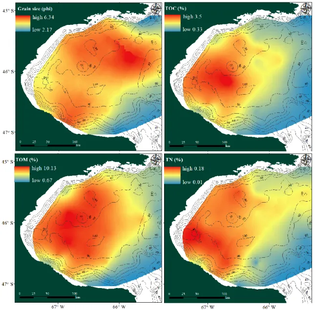
Grain size distribution in San Jorge Gulf (Fig. 2) showed that close to headlands coarse sediments predominated while in the central region fine sediments were present. This distribution pattern of environmental variables followed the spatial variation in depths. In this context, total organic matter, total organic carbon and total nitrogen presented higher proportions associated with fine sediment in the central region while they radially decreased towards the headlands.
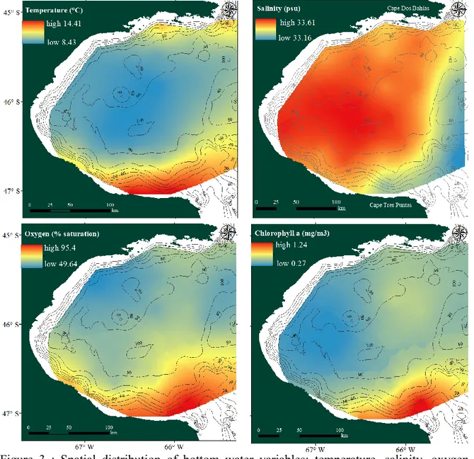
Considering bottom water variables distribution in San Jorge Gulf, a depth-related spatial pattern was also observed (Fig. 3). In the central region, temperatures presented low values that increased towards the headlands, while salinity followed the opposite pattern. Particularly, bottom water in the South close to Cape Tres Puntas showed higher temperature and lower salinity. The mouth of the SJG also presented lower salinity values. Oxygen concentrations were highest close to headland in the South and decreased with depths. Chlorophyll a presented the highest concentrations close to Cape Tres Puntas.
22
Figure 2 : Spatial distribution of sediment variables: gran size, total organic matter (TOM), total organic carbon (TOC) and total nitrogen (TN). Bathymetry is indicated by isolines.
Figure 3 : Spatial distribution of bottom water variables: temperature, salinity, oxygen availability and chlorophyll a. Bathymetry is indicated by isolines.
24
CORRELATION BETWEEN ENVIRONMENTAL VARIABLES
The PCA for INIDEP data highlighted two dimensions that might explain together 81.6% of the total variability (Fig. 4 and Table 2). The PC1 axis explained 71.7% while the second dimension explained 9.9% of the variability. Oxygen, chlorophyll a and TOM were associated with the first PCA axis, while temperature, depth, bottom current, TN, salinity, grain size and TOC showed a closer association with the second PCA axis. Particularly, TOC and TN showed similar direction as descriptors. These variables might be highly correlated.
Figure 4 : Principal component analyses plots with the first two axes for INIDEP data. Stations (objects) and environmental variables (descriptors) are represented. Vectors indicate the direction and strength of environmental variables.
Regarding stations (objects) and environmental variables (descriptors), it was possible to observe that stations close to Cape Tres Puntas (indicated with red circle)
these stations presented higher concentrations of oxygen and chlorophyll a. Stations close to the coast in the inner part of the gulf (indicated with orange circles) presented fine sediments, high TOM and TOC concentrations, temperature and oxygen availability. Stations offshore (indicated with green circle) were positively associated with depths and salinity. Stations in the central region (indicated with blue circle) present fine sediments, high concentrations of TOM, TOC and TN, and bottom water is cold with low availability of oxygen and chlorophyll a concentration (Fig. 4).
Table 2 : Results from PCA considering INIDEP environmental data.
PC 1 PC 2 Eigenvalues 7.17 0.991 Variance explained (%) 71.7 9.9 Eigenvectors Depth -0.293 0.487 TOM -0.349 -0.181 TOC -0.325 -0.322 TN -0.330 -0.375 Temperature 0.343 -0.194 Salinity -0.336 0.161 Oxygen 0.343 -0.102 Chlorophyll a 0.294 0.076 Grain size -0.289 -0.379 Bottom current 0.244 -0.512
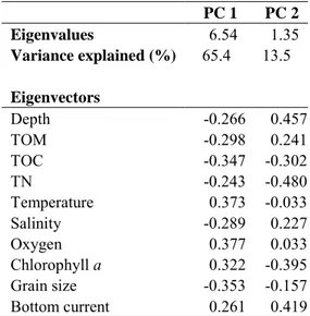
The PCA for MARES data highlighted two dimensions that explained together 78.9% of the variability (Fig. 5 and Table 3). The PC1 axis explained 65.4% while the second axis explained 13.5% of the variability. Oxygen, temperature and grain size were associated with the first PCA axis while TN, TOC, depth, chlorophyll a, bottom current and TOM were associated with the second PCA axis. Particularly, salinity and TOM showed similar direction as descriptors. These variables might be highly correlated.
26
Figure 5 : Principal component analyses plots with the first two axes for MARES data. Stations (objects) and environmental variables (descriptors) are represented. Vectors indicate the direction and strength of environmental variables.
Regarding stations (objects) and environmental variables (descriptors), higher heterogeneity was observed among stations from MARES mission than from the INIDEP data. The station close to Cape Tres Puntas (indicated in red circle) presented coarse sediments, high concentrations of chlorophyll a and high temperature (Fig. 5), following the pattern described for stations in this area in Figure 4. Stations in the mouth (indicated purple circle) appeared to be related with bottom current and oxygen concentrations. The rest of the stations were associated with fine sediments and cold bottom waters with less availability of chlorophyll a, but they showed high heterogeneity (Fig. 5). Stations close to coasts (indicated with orange circles) were associated with similar gran size and TOC conditions. Stations in the central region (indicated with blue circle) present fine sediments,
chlorophyll a concentration (Fig. 5).
Table 3 : Results from PCA considering MARES environmental data.
PC 1 PC 2 Eigenvalues 6.54 1.35 Variance explained (%) 65.4 13.5 Eigenvectors Depth -0.266 0.457 TOM -0.298 0.241 TOC -0.347 -0.302 TN -0.243 -0.480 Temperature 0.373 -0.033 Salinity -0.289 0.227 Oxygen 0.377 0.033 Chlorophyll a 0.322 -0.395 Grain size -0.353 -0.157 Bottom current 0.261 0.419
1.5.2BENTHIC DIVERSITY AND RELATIONS WITH BENTHIC ENVIRONMENT
Results are presented for epifauna taxonomic and functional diversity, and then for infauna taxonomic and functional diversity. In addition, the relations between assemblages and environmental variables are indicated in each section.
TAXONOMIC EPIFAUNA DIVERSITY
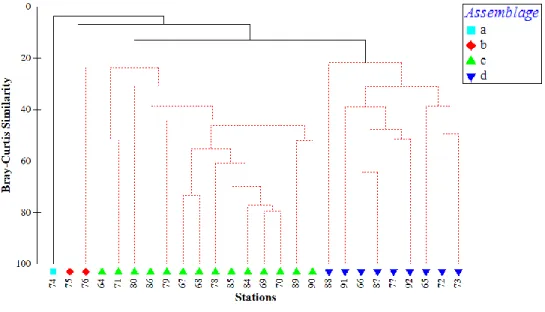
Cluster and SIMPROF analysis on epifauna data identified four groups (Fig. 6). Assemblage a has been identified with data from only one station, at the southern coast (Fig. 7). Assemblage b was found close to Cape Tres Puntas. Assemblage c was present in
28
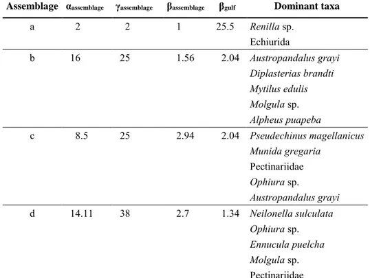
the central and western area. Assemblage d was found in the North, close to the mouth and southern coastal area (Mazarredo). The γgulf diversity identified 51 epifauna taxa (Table 4; see Table S3 for assemblages’ composition). Differences between assemblages were mainly explained by presence or abundance of Pseudechinus magellanicus, Neilonella
sulculata, Ennucula puelcha, Munida gregaria, Renilla sp., Austropandalus grayi, Mytilus edulis and Diplasterias brandti (Table S4).
Figure 6 : Taxonomic cluster based on Bray-Curtis Similarity matrix using epifauna taxonomic abundance by station. The taxonomic epifauna assemblages are represented with different colors.
Assemblage a showed the lowest diversity, with only two taxa, Echiurida and Renilla sp. (Table 4). Assemblage b presented the highest αassemblage. However, the βassemblage indicated that the variation between stations from this assemblage was high. Assemblage b was characterised by A. grayi, D. brandti, M. edulis, Molgula sp. and Alpheus puapeba. The SIMPER analyses indicated that D. brandti, A. grayi, Cirolana sp., Hemioedema
spectabilis, Carolesia blakei and Boltenia sp. contributed 93.62% to the average similarity
Figure 7 : Location of epifauna taxonomic assemblages in the SJG.
Assemblage c was characterised by high abundances of P. magellanicus, M.
gregaria, Pectinariidae sp., Ophiura sp. and A. grayi. The SIMPER analyses indicated that P. magellanicus, M. gregaria, Pectinariidae, Notiax brachyophthalma and Pterysgosquilla armata armata contributed 90.68% to the average similarity of 41.22 (Table S4).
Assemblage d presented the highest γassemblage. This assemblage was characterised by
high abundances of N. sulculata, Ophiura sp., E. puelcha, Molgula sp. and Pectinariidae. The SIMPER analyses indicated that N. sulculata, E. puelcha, Molgula sp., M. gregaria, P.
armata armata, Pandora cistula, N. brachyophthalma and Peachia sp. contributed 90.49%