Université de Montréal
Bayesian Modeling of Biological Motion Perception in
Sport
Modélisation bayésienne de la perception du mouvement
biologique dans le sport
par Khashayar Misaghian
École d’optométrie
Thèse présentée
en vue de l’obtention du grade de doctorat en Sciences de la Vision
option Neurosciences de la vision et psychophysique
Janvier 2020
Résumé
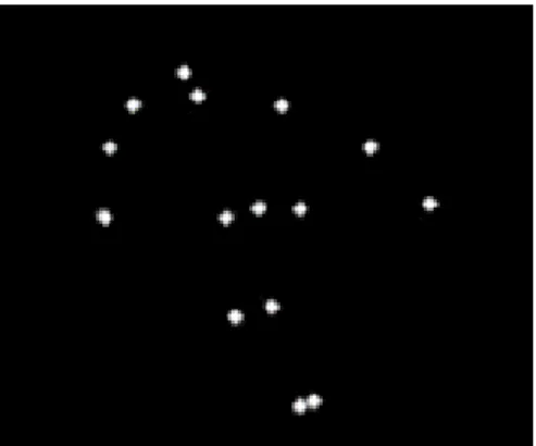
La perception d’un mouvement biologique correspond à l’aptitude à recueillir des informations (comme par exemple, le type d’activité) issues d’un objet animé en mouvement à partir d’indices visuels restreints. Cette méthode a été élaborée et instaurée par Johansson en 1973, à l’aide de simples points lumineux placés sur des individus, à des endroits stratégiques de leurs articulations. Il a été démontré que la perception, ou reconnaissance, du mouvement biologique joue un rôle déterminant dans des activités cruciales pour la survie et la vie sociale des humains et des primates. Par conséquent, l’étude de l’analyse visuelle de l’action chez l’Homme a retenu l’attention des scientifiques pendant plusieurs décennies. Ces études sont essentiellement axées sur informations cinématiques en provenance de différents mouvements (comme le type d’activité ou les états émotionnels), le rôle moteur dans la perception des actions ainsi que les mécanismes sous-jacents et les substrats neurobiologiques associés.
Ces derniers constituent le principal centre d’intérêt de la présente étude, dans laquelle nous proposons un nouveau modèle descriptif de simulation bayésienne avec minimisation du risque. Ce modèle est capable de distinguer la direction d’un ballon à partir d’un mouvement biologique complexe correspondant à un tir de soccer.
Ce modèle de simulation est inspiré de précédents modèles, neurophysiologiquement possibles, de la perception du mouvement biologique ainsi que de récentes études. De ce fait, le modèle présenté ici ne s’intéresse qu’à la voie dorsale qui traite les informations visuelles relatives au mouvement, conformément à la théorie des deux voies visuelles. Les stimuli visuels utilisés, quant à eux, proviennent d’une précédente étude psychophysique menée dans notre
et en ajustant une série de paramètres, le modèle proposé a été capable de simuler la fonction psychométrique ainsi que le temps de réaction moyen mesurés expérimentalement chez les athlètes.
Bien qu’il ait été établi que le système visuel intègre de manière optimale l’ensemble des indices visuels pendant le processus de prise de décision, les résultats obtenus sont en lien avec l’hypothèse selon laquelle les indices de mouvement sont plus importants que la forme dynamique dans le traitement des informations relatives au mouvement.
Les simulations étant concluantes, le présent modèle permet non seulement de mieux comprendre le sujet en question, mais s’avère également prometteur pour le secteur de l’industrie. Il permettrait, par exemple, de prédire l’impact des distorsions optiques, induites par la conception de verres progressifs, sur la prise de décision chez l’Homme.
Mots-clés : Mouvement biologique, Bayésien, Voie dorsale, Modèle de simulation
Abstract
The ability to recover information (e.g., identity or type of activity) about a moving living object from a sparse input is known as Biological Motion perception. This sparse input has been created and introduced by Johansson in 1973, using only light points placed on an individual's strategic joints. Biological motion perception/recognition proves to play a significant role in activities that are critical to the survival and social life of humans and primates. In this regard, the study of visual analysis of human action had the attention of scientists for decades. These studies are mainly focused on: kinematics information of the different movements (such as type of activity, emotional states), motor role in the perception of actions and underlying mechanisms, and associated neurobiological substrates.
The latter being the main focus of the present study, a new descriptive risk-averse Bayesian simulation model, capable of discerning the ball’s direction from a set of complex biological motion soccer-kick stimuli is proposed.
Inspired by the previous, neurophysiologically plausible, biological motion perception models and recent studies, the simulation model only represents the dorsal pathway as a motion information processing section of the visual system according to the two-stream theory, while the stimuli used have been obtained from a previous psychophysical study on athletes. Moreover, using the psychophysical data from the same study and tuning a set of parameters, the model could successfully simulate the psychometric function and average reaction time of the athlete participants of the aforementioned study.
Although it is established that the visual system optimally integrates all available visual cues in the decision-making process, the results conform to the speculations favouring motion cue importance over dynamic form by only depending on motion information processing.
As a functioning simulator, the present simulation model not only introduces some insight into the subject at hand but also shows promise for industry use. For example, predicting the impact of the lens-induced distortions, caused by various lens designs, on human decision-making.
Keywords : Biological motion, Bayesian, Dorsal pathway, Hierarchical simulation model,
Table des matières
RÉSUMÉ ... 2
ABSTRACT ... 4
TABLE DES MATIÈRES ... 6
LISTE DES TABLEAUX... 9
LISTE DES FIGURES ... 10
LISTE DES SIGLES ... 15
REMERCIEMENTS... 17
INTRODUCTION ... 18
EARLY INSPIRATIONS FOR COMPUTATIONAL BRAIN MODELS ... 18
HOW TO TACKLE THE PROBLEM OF COMPUTATIONAL MODELING? ... 18
Implementation Level ... 20
Representational and Algorithm Level. ... 20
MODELING CIRCUIT MECHANISMS AND NEURAL DYNAMICS OF DECISION-MAKING ... 21
Decision Making as a Proof of Life ... 21
There Will Be Uncertainty ... 22
Brain: Our Statistical Decision-Making Machine ... 23
More Practical Definition of Decision-Making ... 23
Modeling of Decision Making ... 24
Neural Correlates of Decision Making ... 27
Signal Detection Theory and Sequential Analysis ... 27
Where Is This Log LR in the Brain? ... 28
It Is Teamwork and It Is Hierarchical to Form the Decision Variable. ... 31
Bounded Integrator Models in Implementation Level. ... 33
It Runs on Inter-Inhibition, Intra-excitation, and Leakage. ... 34
State-Space Interpretation. ... 35
Hypotheses on Modeling SAT at the Implementation Level. ... 37
Modulation of the encoding of evidence. ... 38 Modulation of the Integration of Evidence, Encoded by the Previous Stage This class of hypotheses has three sub-classes: 1. Modulation of the rate of integration, 2. Modulation of the onset of integration, and 3. Modulation of
Modeling Behaviour. ... 42
PRESENT STUDY ... 42
Why Biological Motion? ... 42
Present State of Modeling of Biological Motion? ... 44
Present Work. ... 46
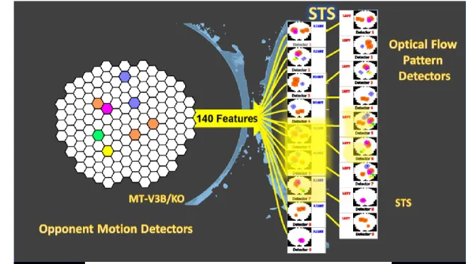
The Anatomy of the Model. ... 47
Local motion energy detectors. ... 48
Opponent-motion detector ... 48
Complex global optic flow patterns. ... 50
Complete biological motion pattern detectors. ... 51
SAT and Our Model. ... 52
ARTICLE 1 ... 53
ABSTRACT ... 54
INTRODUCTION ... 55
MODEL ... 57
Local Motion Energy Detectors. ... 58
Opponent-motion detectors. ... 58
Complex Global Optical-Flow Patterns. ... 59
Complete Biological Motion Pattern Detectors (Motion Pattern Detectors). ... 61
Robust Mutual Inhibition Model. ... 62
Modeling of the Internal Noise. ... 63
METHODS ... 65
Stimuli and Data. ... 65
Local Motion Energy and Opponent Motion Neurons. ... 66
Optic Flow Pattern Neurons. ... 66
Motion-Pattern Neurons. ... 67
Simulating Human Behaviour. ... 69
RESULTS ... 69
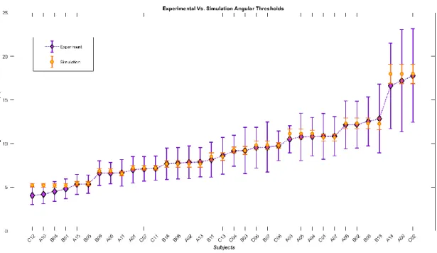
Human Results Vs. Simulation Results. ... 72
DISCUSSION... 75
FUNDING ... 76
ARTICLE 2 ... 77
ABSTRACT ... 78
MODEL ... 81
Local Motion Energy Detectors. ... 82
Opponent-Motion Detectors. ... 82
Complex Global Optic Flow Pattern Detectors. ... 83
Complete Biological Motion Pattern Detectors (Motion Pattern Detectors). ... 83
Robust Mutual Inhibition Model with Adaptation. ... 84
Modeling Internal Noise. ... 85
METHODS ... 86
Local Motion Energy and Opponent Motion Neurons. ... 87
Optic Flow Pattern Neurons. ... 88
Motion Pattern Neurons. ... 88
Operating the Simulator. ... 88
RESULTS ... 89
Extended Model Reaction Time Output. ... 89
Integration of Rotation Detection in Opponent Motion Hierarchy Level. ... 92
Human Results Vs. Simulation Results. ... 93
DISCUSSION... 95
FUNDING ... 96
CONCLUSION ... 97
ONLINE LEARNING ... 98
MORE ON AUTISM ... 101
REACTION TIME APPROXIMATION ... 101
APPLICATIONS OF THE EXTENDED DESCRIPTIVE RISK-AVERSE BAYESIAN MODEL ... 102
ANNEX I: MODEL OUTPUTS FOR RANGES OF ALL PARAMETERS ... I ANNEX II: MODELS SCHEMATICS ... I
Liste des tableaux
Table02-1: by tuning the 𝑘, 𝜏 and 𝛿 Parameters the angular thresholds (75%) and the slopes of athletes’ psychometric functions have been simulated……….… .59 Table03-1: For 𝜏𝑎 = 1.22, the angular threshold and slope of the psychometric function and the average reaction time of the model for different values of 𝜏 and 𝑘, for two noise levels (𝛿 = 0.030 and 𝛿 = 0.034) have been calculated and reported below………78 Table03-2: by tuning the 𝑘, 𝜏, 𝛿 and 𝜏𝑎 the angular thresholds (75%) and the slopes of athletes’ psychometric functions along with their average reaction times have been simulated………..81
Liste des figures
Figure 1-1: Marr's levels of analysis (Commons, 2018) ... 19
Figure 1-2: Example graph of accumulation of evidence in a Drift-Diffusion Model, with a source at 100% noise (Commons, 2017) ... 26
Figure 1-3: The ball is the current state of the system, and the curve is the energy landscape of the neural model, T is the target the low-energy, attractor and D is the other low-energy attractor, the distractor. The vertical arrow represents the onset of the stimulus and how this change could drive the system towards each of these steady-state attractors (Standage et al., 2014) ... 36
Figure 1-4: From left to right, 1. The evidence-encoding stage, 2. The integration stage, 3. The Thresholding Stage (Standage et al., 2014) ... 36
Figure 1-5: Modulation of the encoding of the evidence (Standage et al., 2014) ... 38
Figure 1-6: Modulation of the rate of integration of evidence (Standage et al., 2014) ... 39
Figure 1-7: Modulation of the onset of integration (Standage et al., 2014)... 40
Figure 1-8: Modulation of the Sensitivity to the Evidence (Standage et al., 2014) ... 40
Figure 1-9: Modulation of the non-integrator signal into the thresholding circuitry (Standage et al., 2014) ... 41
Figure 1-10: Connectivity Modulation between Integrators and Thresholding stage (Standage et al., 2014) ... 41
Figure 1-11: A frame from a soccer kick biological motion stimulus ... 43
Figure 1-12: Schematics of how the stimuli were produced. The connecting lines or the ball were not present at the actual stimuli (Romeas & Faubert, 2015) ... 47
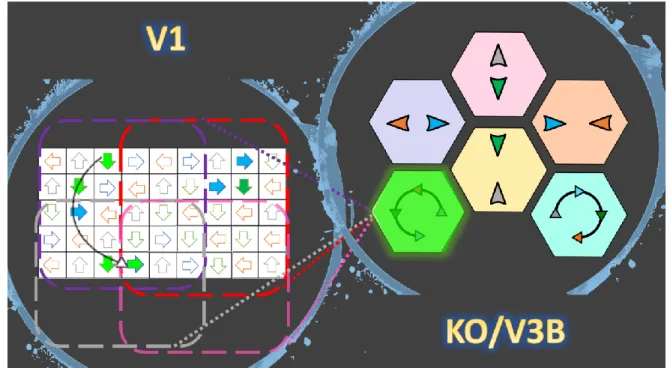
Figure 1-13: Each white square with an arrow represents a neuron sensitive to the direction that its arrow direction. Two areas show the reflection of two moving dots on the retina and, therefore, on V1. As the dots pave their paths, if there exists a sensitive neuron would fire and get deactivated as the stimulus passes. Here, for the sake of demonstration, we kept all the stimulated neurons active on the right side of the picture. ... 48 Figure 1-14: The color-filled arrows in the white square boxes demonstrate the activated local motion detectors at one point in time. The hexagons on the right represent an ensemble of opponent motion detectors at a higher level in the visual system. The counter clock-wise
(depicted by dotted lines) are experiencing the anticipated motions at this point in time, in this example. ... 49 Figure 1-15: On the right, there is an exemplary 140-element feature vector made by opponent motion neurons in which white means no activity and colors represent different quantities (sparse for the demonstration purposes). On the right, there are 18 complex global flow pattern detectors 9 for the right kicks and 9 for the left kicks inside each of these neurons; there is a template stored. The more similar the input is to the templates the larger is the feed-forward input of that neuron (depicted by neon yellows of different intensity). From the picture one could assume that the presented feature vector represents the seconds 41 to 50 of the right side kick stimulus sequence (the detector 4 of the right kick group has the most intense yellow) while the detector 4 of the left kick group falsely shows some activity. It is up to the thresholding stage to receive the integrated evidence to make the final decision. ... 51 Figure 1-16: The anatomy of the interaction between two decision making neurons (or group of neurons). The round headed shape connections (blue and pink) represent the existing mutual inhibitions. “R” marks the neuron (or group of neurons) that gets activated if the decision is “to the right” and “L” marks the neuron (or group of neurons) that gets activated in case the decision is “to the left”. ... 52 Figure 2-1: Schematic of the model in one hypothetical point in time, from left to right: (a) the reel of biological motion stimulus (b) local motion detectors as ensemble of 1116 neurons positioned in a 36 by 31 arrangement, are firing due to the motions they have experienced during two consecutive frames, represented by the cells with filled-color arrows (blue: right, orange: left, grey: up, and green: down), the larger, two-headed, colorful arrows were drawn to display the types of opponent motions that would be sensed on the next level (cyan: horizontal expansion, orange: vertical expansion, and magenta: vertical contraction) (c) opponent motion detectors, the ensemble of 100 neurons to detect horizontal expansion, horizontal contraction, vertical expansion, and vertical contraction, the activated detectors are marked with color-filled hexagons with their corresponding color (cyan: horizontal expansion, orange: vertical expansion, and magenta: vertical contraction), (d) optical-flow pattern detectors, an arrangement of 18 neurons following a one-dimensional mean-field dynamics, each neuron incorporates a statistical template (displayed as colorful map) that represents a specific part of the manifold of the kicking sequences (for example neuron number 2 contains a template for the seconds 11 to
20 of the kick-to-right sequence, while neuron number 10 would have a larger instantaneous input for the seconds 1 to 10 of the kick to the left stimulus). Green arrows are highlighting the contribution of two cells to the evidence integration at that hypothetical point due to the similarity of the evidence signal and their template (e) thresholding stage, two decision neurons for the right and left decisions (marked by capital letters R and L on the square cells with soft edges) are following our mutual inhibition dynamics receiving their corresponding inputs from integration stage, the straight and curve lines with rounded heads highlight the inhibitory interaction between the neurons and the auto-inhibition, respectively. No activity could be seen by either of the neurons since at that hypothetical point in time, neither made a decision yet. 64 Figure 2-2: The activity of these neurons in the absence of the internal noise to the stimulus representing a kick with 9°degrees of deviation to the right. Neurons 1 to 9 are responsive to the right-side kicks and neurons 11 to 18 are sensitive to the left-side kicks. ... 67 Figure 2-3: The neuron responsive to the right-side kick (blue) is highly activated, while the inhibition in the other neuron is evident. ... 68 Figure 2-4: The psychometric function angular thresholds resulted from running the model for exemplary ranges of neuronal latency ( 𝜏 = 0.024, 0.025, 0.03, 0.033, 0.037 𝑠𝑒𝑐) and inhibitory gain (𝑘 = 2, 4, 8, 16, 32) for three noise levels (𝛿 = 0.028, 0.030, 0.034) ... 70 Figure 2-5: The psychometric function slopes resulted from running the model for exemplary ranges of neuronal latency ( 𝜏 = 0.024, 0.025, 0.03, 0.033, 0.037 𝑠𝑒𝑐) and inhibitory gain (𝑘 = 2, 4, 8, 16, 32) for three noise levels (𝛿 = 0.028, 0.030, 0.034) ... 71 Figure 2-6: diamonds represent the angular thresholds (75%) calculated from the psychometric function of the subjects in the experimental tests and the black dots display the angular thresholds generated by simulation. ... 74 Figure 2-7 : Diamonds represent the slopes of the subjects’ psychometric functions while black dots demonstrate the simulated slopes ... 74 Figure 3-1: Schematic of the model in one hypothetical point in time, from left to right: (a) the reel of biological motion stimulus (b) local motion detectors as ensemble of 1116 neurons positioned in a 36 by 31 arrangement, are firing due to the motions they have experienced during two consecutive frames, represented by the cells with color-filled arrows (blue: right, orange:
display the types of opponent motions that would be sensed on the next level (cyan: horizontal expansion, orange: vertical expansion, magenta: vertical contraction, green: counter-clockwise rotation, and yellow: clockwise rotation) (c) opponent motion detectors, the ensemble of 140 neurons to detect horizontal expansion, horizontal contraction, vertical expansion, and vertical contraction, the activated detectors are marked with color-filled hexagons with their corresponding color (cyan: horizontal expansion, orange: vertical expansion, magenta: vertical contraction, green: counter-clockwise rotation, and yellow: clockwise rotation), (d) optical-flow pattern detectors, an arrangement of 18 neurons following a one-dimensional mean-field dynamics, each neuron incorporates a statistical template (displayed as colorful map) that represents a specific part of the manifold of the kicking sequences (for example neuron number 2 contains a template for the seconds 11 to 20 of the kick-to-right sequence, while neuron number 10 would have a larger instantaneous input for the seconds 1 to 10 of the kick to the left stimulus). Green arrows are highlighting the contribution of two cells to the evidence integration at that hypothetical point due to the similarity of the evidence signal and their template (e) thresholding stage, two decision neurons for the right and left decisions (marked by capital letters R and L on the square cells with soft edges) are following our mutual inhibition dynamics receiving their corresponding inputs from integration stage, the straight and curve lines with rounded heads highlight the inhibitory interaction between the neurons and the auto-inhibition, respectively. No activity could be seen by either of the neurons since at that hypothetical point in time, neither made a decision yet. Also, the dotted curved arrows and the circle with the letter D, are the representatives of the disremembering mechanism. ... 85 Figure 3-2 : Subfields in one clockwise rotation receptive field of our model... 87 Figure 3-3: The reaction times resulted from running the model for exemplary ranges of neuronal latency ( 𝜏 = 0.024, 0.025, 0.03, 0.033, 0.037 𝑠𝑒𝑐) and inhibitory gain (𝑘 = 2, 4, 8, 16, 32) for three noise levels (𝛿 = 0.028, 0.030, 0.034) ... 90 Figure 3-4: Diamonds represent the average reaction time of athlete sub-groups performing the tasks in the psychometric experiment (Romeas & Faubert, 2015) while dots demonstrate the average reaction times acquired from the model simulating those sub-groups. ... 95 Figure 4-1 : A simple example of one episode of the Q-learning algorithm for a 3 state system with an absorbing goal ... 100
Figure 4-2 : From left to right: animated visual input, the lens design model, local motion detection layer, opponent motion detection layer, global pattern detection layer, complete biological motion detection layer... 103 Figure 4-3 : Above are three frames from one stimulus and below are the corresponding aberrated frame with barrel aberration of 2.3 diopters ... 104
Liste des sigles
3D : Three Dimensional
STS : Superior Temporal Sulcus V1/2 : Visual Areas 1 and 2 MT : Medial Temproal Area MST : Medial Superior Temporal KO : Kinetic Occipital
V3B : Ventral 3 Area B SD: Standard Deviation
Remerciements
First off, I would like to express my deepest gratitude to my advisor Prof. Jocelyn Faubert for his trust and continuous support, none of this would have had happened without him. His mentorship not only helped me in my research but also guided me in all other areas of my life. I could not have imagined having a better advisor and mentor for my PhD study.
Additionally, I must thank my other dear advisor, Dr. Eduardo Lugo, for his encouragement, patience and specifically his immense knowledge. His counsel was integral to the existence of the present study.
Maman, Baba and Parisi, thanks for all the love you have given me since Day One, Without your support, doing this doctorate would not have been possible. I love you all.
I will be forever grateful to the fellows from the lab for their support, especially: Dr. Delphine Bernardin, Raphael Doti, Vadim Sutyuchev, Marie Maze, Sergio Mejia, Yannick Roy, Thomas Romeas, Robyn Lahiji, Laura Mikula. Also, friends and fellows from the department: dearest Umit Keysan, Bruno Oliveira, Nelson Cortes, Sabine Demosthènes, Sylvie Beaudoin.
Last but not least, my greatest love and appreciation to my friends who were there for me during this journey: Marie-Claude Légaré, Sajjad Ghaemi, Amir Pourmorteza, Ali Seyedi, Behzad Barzegar, Reza Maghsoudi.
Introduction Early Inspirations for Computational Brain Models
In 1973 Alan Newell argued that the scientific trend in the field of psychology and cognitive science must reach beyond mere reductionism. Despite all functional aspects of reductionism, he believed that endeavours should lead to a unified knowledge integrated into a unified human-information processing model that could perform generalized tasks and could explain the exploitation and the synergy of the brain’s sub-functions (Kriegeskorte & Douglas, 2018; Newell, 1994).
On the other hand, the advent of ground-breaking imaging techniques like fMRI gave rise to the field of cognitive neuroscience, which succeeded in mapping the global functional layout of the brain, initially by associating task-related activations to the brain regions.
Despite its high importance, one could not discover the related cognitive mechanism and subfunctions of the brain using such experimental manipulations in imaging. The reason is implicit in the reverse-inference problem which states that, since a variety of processes could be employed in the brain to accomplish a particular task, one could not infer the underlying cognitive processes based on an experimental manipulation or, in simple words, there is more than one cause for the same effect (Poldrack, 2006). So, no matter how advanced or high resolution the brain maps are, they could not unveil the underlying computational mechanisms due to the nature of the reverse-inference problem.
Ultimately, a computational brain model could be envisioned as a model made up of biologically plausible components, which perform complicated cognitive tasks to re-enact behavior while using data from cognitive science or psychophysical experiments as criteria to corroborate, reject or fine-tune its foundations and functions.
How to Tackle the Problem of Computational Modeling?
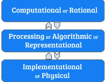
Marr introduced the notion of levels of analysis, stating that the analysis (?) of a complex system should be conducted at different levels: computational, algorithmic and at an implementation level. Also, Marr believed that one should not proceed to a higher (?) level of
At the computational level, the concern is focused on the function of the system (definition of the task) and why it is necessary to execute such a function or performance (the goal of computation). Then, at the algorithmic or representational level, one must investigate how the system executes what it executes, in other words, how inputs are being represented and then manipulated to the outputs. Furthermore, at the implementation level, the question is how to materialize what we learned on the algorithmic level to replicate the function of the system (Kriegeskorte & Douglas, 2018; Marr & Poggio, 1976).
Generally, Marr’s taxonomy provided a robust framework for intuitively describing models of perception and cognition. This is because, first, the insights from a higher level keep the researcher from pursuing redundant questions on lower levels and, second, studying the system on all levels in this way embodies the connection between experimental and theoretical findings in neuroscience (Poggio, 2012).
Subsequently, Poggio, the coauthor of the original hypothesis, made an amendment to the tri-level manifesto of the late Marr, arguing that to understand and be able to describe how an organism learns from its experience in the real world might be even more critical and insightful than the characterization of what that organism has learned in detail. Therefore, he proposed a new level to be added above the computational level, called learning (Poggio, 2012).
Implementation Level
In order to create a realistic neural code from this viewpoint, one must consider the fact that neurons work together. So, to discover a neural code close to realism means to reveal how these neurons co-function. Observations of stereotyped patterns across the cortex which lead to the theory of repeated motifs of cortical microcircuits (Creutzfeldt, 1977) inspired some models that tried to explain the dynamics of a population of neurons, namely, mean field and neural mass models which were, in fact, systems of ordinary differential equations (Coombes, 2010). One of the more recent and more realistic neural-population dynamic models of this kind is the canonical microcircuit model that incorporates more details such as local recurrences in its dynamic (Bastos et al., 2012).
One common exciting fact about all these models, from the most simple to the most complex, is the importance of the balance of inhibition and excitation between neurons which appeared to be a theme in the more recent studies, suggesting that an efficient neural code essentially requires a tight excitation and inhibition balance (Denève & Machens, 2016).
However population-dynamics models are not showing much promise when it comes to explaining the interactions between cortical regions. Therefore, neuroscience resorts to connectivity models such as structural connectivity and functional connectivity models from which the graph-theoretic measures could be generated using thresholding, which shows the connection hubs between different regions of the brain. However, such models can not include latencies as well as indirect connectivities between brain regions (Sporns, 2007).
Finally, effective connectivity methods are biologically plausible; they take latencies and indirect inter-regional connections into account. The idea is that one biophysical model like the canonical microcircuit and one measurement model like lead field model (if we are dealing with EEG data) is being assigned to each region under investigation, and from that a wide range of dynamics in EEG, fMRI and other forms of data could be described or generated. Nonetheless, they are built on mean overall activations of the regions and generally are not suitable to perform actual cognitive tasks (Stephan & Friston, 2010).
to cognitive processes, responses or even stimuli. In other words, the objective is how neurons represent and process the information. In that regard encoding and decoding models exist: encoding models use the features from the stimuli to predict the brain responses, whereas decoding models try to predict the aspects of the stimuli from brain activation patterns. Other than stimulus reconstruction, a decoding model could contribute to understanding the representational content of a fine grain pattern or shed light on which areas between task and response contain mutual information (Diedrichsen & Kriegeskorte, 2017).
Moreover, algorithm-based models like, neural network models, reinforcement learning, Bayesian models also belong to this level of analysis. Neural networks have been used as brain computational models in recent years to explain or predict human behaviour and brain activity data and to perform high-level tasks (Kriegeskorte, 2015). The convolutional recurrent network which incorporated long-range connections into its architecture inspired by structural connectivities in the brain to model object recognition in the visual system (Nayebi et al., 2018), and canonical microcircuit based models within Bayesian framework in the work of (Moran, Pinotsis, & Friston, 2013) are two more recent examples.
Modeling Circuit Mechanisms and Neural Dynamics of Decision-making Decision Making as a Proof of Life
Biologists make the assertion that “life is irritable.” Therefore, an entity is considered a living organism as long as it creates a purposeful response to the environment’s stress that impacts it. One thoughtful, resolute response to a situation indeed entails the concept of decision making. According to this view, the act of decision making is one common thing among all living things (Dobransky, 1999).
Unlike a rock that does nothing actively in response to its surroundings, a frog decides to hop away from the predator, a tree grows its branches towards light and not the shade, and these are all decisions made in response to what presented by the environment. On the human level, decisions are what renders each person’s identity without equal on earth and that identity comes from nothing but the sum of all and every single decision ever made until that time point by that person (Dobransky, 1999).
The above could shed some light on the importance of decisions and, consequently, their mechanisms in every aspect of the lives of living organisms.
There Will Be Uncertainty
Decision-making could be viewed as an act of finding a solution to a problem (presented by the environment). The solution has to be satisfactory or even better: optimal. Such a process could be based on the agent’s knowledge of explicit or tacit nature, while the result would be rational or irrational (Brockmann & Anthony, 2002). Furthermore, finding a solution could be construed as a simple act of choosing an alternative among multiple alternatives. Reality dictates that different circumstances could lead to different results and, the more of them there are, the less certain would the agent be about the outcomes. So, one could say that the nature of the events in our universe begets uncertainty in making a decision, and that is why choice under uncertainty is the core of decision theory.
Decision theory dates back to the 17th century when Pascal introduced the notion of expected value as a criterion for making a decision in the sense that, by knowing the value of each outcome and its probability and by multiplying these two numbers, one has the expected value of each result and could simply choose the one with the highest value as the winning alternative. In the following century, Bernoulli, using the St. Petersburg Paradox, argued that such a solution to the problem of decision making is suboptimal and, to resolve this conundrum, he introduced the expected utility hypothesis which asserts that only counting on expected value would not suffice and other factors like the agent’s wealth, the diminishing marginal benefit and the cost of entering the game must be taken into consideration in the form of one utility function. Thereupon, the agent could make an optimal decision (Schoemaker, 1982).
The resurfacing of the Bayesian probability theory in the 20th century extended the capacities of the expected utility theory and “expected utility maximization” was able to explain some rational behaviours, (Von Neumann, Morgenstern, & Kuhn, 2007). Later, Maurice Allais and Daniel Ellsberg demonstrated systematic deviation from expected-utility maximization in many human behaviors. After that, the prospect theory renewed the experimental economic behavior studies, introducing three distinct regularities in human decision making (Allais &
2. The agent has more focus on changes in the utility rather than the actual utilities 3. The initial piece of information offered to the agent at the beginning of the process critically affects its estimation of subjective probabilities
Ultimately, it is safe to say that the process of decision making is a statistical phenomenon and any effort to explain or model such a process must indeed capture its essence of randomness.
Brain: Our Statistical Decision-Making Machine
So far, we believe that our nervous system, with the brain as its chief, is in charge of the decisions that we make. Even though establishing decision-making as a statistical process does not entail that decision-making happens in the same fashion in the brain, a wide range of evidence and the hypotheses built upon it consolidates the idea that the brain is, in fact, a statistical computation machine. For instance, using the logarithm of the likelihood ratio of alternatives as a single quantity that could incorporate many aspects of a statistical decision variable over time, researchers have proposed neural computations that could explain the categorical decisions about sensory stimuli and their substrata in the brain based on electrophysiological studies (Gold & Shadlen, 2001, 2007).
As another example, one recent study suggests that the feeling that one gets after making any decision is called “confidence” in the decision. The results indicate that despite the subjective essence of this notion of confidence, as a matter of fact, it depends on objective statistical calculations (Sanders, Hangya, & Kepecs, 2016).
These are just two primary examples of how the neural computations taking place in the brain are parallel to statistical calculations. Therefore, not only that uncertainty is a significant natural element embedded in the decision-making process but, also, the agent, being the brain, calculates probabilities to achieve a final decision. Considering these notions, the path to model the decision making on any level is clearer. However, to make a good start, one should examine the process on a deeper level.
More Practical Definition of Decision-Making
When it comes to defining the process of decision-making, everyone automatically recalls only the act of choosing, but this process in living creatures in its entirety is a concept beyond that. A good explanation of the organic process of decision-making is: forming a
judgment about an issue of certain difficulty under various conditions of exigency and risk. In other words, the decision-maker happens to make the right decision about an identical problem for a different range of urgency and risk situations. For example, one has to cross a highway with fast-moving cars while being chased by wild dogs or has to pass the very same road with the same fast cars being rewarded for the most nimble performance at its best convenience. Moreover, a long history of behavioral studies corroborates this intuitive notion that decisions are less accurate when conditions side with speed and are more accurate when they favour accuracy, also referred to as speed-accuracy trade-off (SAT)(Fitts, 1966; Standage, Blohm, & Dorris, 2014; Wickelgren, 1977). At the same time, there is often the element of risk involved in every quotidian decision and, not surprisingly, has been a matter of investigation in a whole diverse spectrum of subjects from cognitive studies to neuro-economics (Braun, Nagengast, & Wolpert, 2011; Dayan & Niv, 2008; Nagengast, Braun, & Wolpert, 2010; Niv, Edlund, Dayan, & O'Doherty, 2012; Shen, Tobia, Sommer, & Obermayer, 2014).
The more elaborate the definition is, the clearer are the features that need to be addressed by proposed models. It also shows what would be the next step towards a more general model beyond what already exists.
Having a rather good definition of the decision-making process facilitates discussion of the ways to model it. First, at the representational level and from there, we could gradually proceed to the implementation level.
Modeling of Decision Making
Given levels of abstraction in modeling, models of decision making are accordingly categorized into algorithmic (representational) and implementation levels (Marr, 1982). Intuitively, all proposed models always fall somewhere between these two ends of the modeling spectrum (Standage et al., 2014). Moreover, interestingly, analytic studies demonstrate that under certain conditions and assumptions, implementation-level models could be deemed equivalent to algorithmic models, which provides a massive degree of flexibility when it comes to having a neural code (Bogacz, Brown, Moehlis, Holmes, & Cohen, 2006).
aggregating total meets a criterion level. The aggregating amount is referred to as a decision variable, while the criterion level is referred to as bound. A higher bound allows for a longer time of evidence integration, which could lead to more accurate decisions due to more information. More precisely, integration low-pass filtering quality helps with averaging the accumulating evidence in the presence of noise either in the neural processes or the evidence itself. So, clearly the more prolonged the integration time, the better the average and the higher the chance of accurate decision (Bogacz, Wagenmakers, Forstmann, & Nieuwenhuis, 2010; Ratcliff & McKoon, 2008; P. L. Smith & Ratcliff, 2004; Standage et al., 2014).
It was mentioned previously that the integration of evidence from alternatives by the model could be conducted in different fashions and that is one ground on which the families of bounded integration algorithmic models are categorized;
• Race models: when the evidence of each alternative is integrated independently from the others
• Drift diffusion models (DDM): when the evidence for each choice serves as evidence against the other (two alternative tasks) (Fig 1-2).
• Competing accumulator models: considered as arbitration between models above; this time, each decision variable associated with its respective alternative gets subtracted by other weighted decision variables.
Only by changing the weights in Competing accumulator models, one could transition from pure race models to absolute DDMs. More importantly, this class of models incorporates multi alternative tasks while it serves as a gateway where the algorithmic level could be interpreted into implementation level (Standage et al., 2014).
It is beneficial to emphasize several points before moving further with the bounded integration modeling at the implementation level: Firstly, the decision variable is not necessarily made up of the input associated with evidence, and, in reality, there exist other inputs besides evidence. For example, inputs that modulate prior probabilities of the evidence. This notion elucidates the distinction between the decision variable and the amount of integrated modulated evidence, albeit the implications in defining the bounded integration framework in which evidence of an alternative and the decision variable seemed interchangeable (Standage et al., 2014); Secondly, it was mentioned that the integration helps with noise reduction but, in reality,
noise is not always white. In other words, the autocorrelation of the noise signal, in reality, is not zero and there would be a correlation time, that could only mean that the benefits of integration depend on the timescale of noise correlations (Standage et al., 2014). Finally, although integration operation pertains to the continuous-time domain, for simplicity here, accumulation of evidence in discrete time is being referred to as integration.
Figure01-2: Example graph of accumulation of evidence in a Drift-Diffusion Model, with a source at 100% noise (Commons, 2017)
Now that some light has been shed on the body of work trying to characterize the computations underlying decision making (Ratcliff & McKoon, 2008; P. L. Smith & Ratcliff, 2004), the leading existing hypotheses on identification of neural correlates of these computations may be examined further (Gold & Shadlen, 2007; Kable & Glimcher, 2009; Schall, 2001).
Neural Correlates of Decision Making Signal Detection Theory and Sequential Analysis
It has been highlighted above that multiple pieces of evidence shall come together in time, for an agent, in order to pick an alternative. This could be all substantiated within sequential analysis as an extension to signal detection theory. According to signal detection theory, to infer whether the signal is present or not makes up two hypotheses: ℎ1, the signal is
present, and ℎ2, the signal is not present. Now, evidence 𝑒 bears on the likelihood of each ℎ1 and ℎ2 to be true. Likelihood of ℎ1 states how likely it is that the ℎ1is true, given 𝑒, (𝑃(ℎ1|𝑒)).
The good news is that, in order to decide which hypothesis is true, we do not necessarily need the exact level of likelihood, but that only the ratio of the two likelihoods, 𝐿𝑅, would suffice to come up with a decision (Gold & Shadlen, 2001, 2007).
(1.1) 𝐿𝑅1,2|𝑒 =
𝑃(ℎ1|𝑒)
𝑃(ℎ2|𝑒)
Therefore, if 𝐿𝑅1,2|𝑒 > 1 , the agent would decide that the signal is present and it is not present,
if the other way around (in case 𝐿𝑅1,2|𝑒 = 1, it will randomly pick one of the hypotheses). Now, if there exists any knowledge on the likelihood of the events prior to the presence of evidence or, in general, any external factor that affects the likelihoods, it is best to adjust the previous formula into a general one (sequential analysis formalization) capable of incorporating such factors. Therefore, the decision goes to ℎ1if (Gold & Shadlen, 2001, 2007):
(1.2) 𝐿𝑅1,2|𝑒 𝑃(ℎ1) 𝑃(ℎ2) = 𝑃(ℎ1|𝑒)𝑃(ℎ1) 𝑃(ℎ2|𝑒)𝑃(ℎ2) > 1
where 𝑃(ℎ1) and 𝑃(ℎ2) are the prior probabilities of the two hypotheses before presenting the agent with any evidence. More interestingly, the rule allows for the integration of multiple independent observations (𝑒1, 𝑒2, …, 𝑒𝑛) (Gold & Shadlen, 2001, 2007):
(1.3) 𝐿𝑅1,2|𝑒1,𝑒2,…,𝑒𝑛 = 𝐿𝑅1,2|𝑒1∙ 𝐿𝑅1,2|𝑒2. … ∙ 𝐿𝑅1,2|𝑒𝑛
Ultimately, to factor in the cost or benefits affiliated with the choices, one would choose the ℎ1 when (Gold & Shadlen, 2001):
(1.4) 𝐿𝑅1,2|𝑒 >
𝑉22− 𝑉21
𝑉11− 𝑉12
where, 𝑉𝑖𝑗is the expected cost of choosing ℎ𝑗 when ℎ𝑖 is true (when 𝑖 = 𝑗 it is a positive reward, and it is a negative cost when 𝑖 ≠ 𝑗). Combining all three equations above that incorporate prior knowledge and cost computing into the process of decision making, the result is (Gold & Shadlen, 2001; D. M. Green & Swets, 1966):
(1.5) 𝐿𝑅1,2|𝑒1∙ 𝐿𝑅1,2|𝑒2∙ … ∙ 𝐿𝑅1,2|𝑒𝑛∙ 𝑃(ℎ1) 𝑃(ℎ2) ∙𝑉11− 𝑉12 𝑉22− 𝑉21 > 1
Here the left side of the equation is what we mathematically refer to as the decision variable and, as one can see, it is not only comprised of likelihood ratios of pieces of evidence.
It is worth mentioning that the formalization is not only limited to two-choice tasks. Instead, it applies to multi-alternative scenarios by calculation and comparison of all the likelihood ratios (D. M. Green & Swets, 1966).
Furthermore, given that applying a monotonic kernel holds the inequality, taking the logarithms of the previous equation yields:
(1.6) 𝑙𝑜𝑔𝐿𝑅1,2|𝑒1+ 𝑙𝑜𝑔𝐿𝑅1,2|𝑒2+ ⋯ + 𝑙𝑜𝑔𝐿𝑅1,2|𝑒𝑛+ 𝑙𝑜𝑔 [𝑃(ℎ1)
𝑃(ℎ2)] + 𝑙𝑜𝑔 [
𝑉11− 𝑉12 𝑉22− 𝑉21] > 0 This form of the decision rule shows how pieces of evidence could be accumulated towards a final decision by simple summation. That is to say, while a positive value is in favour of accepting the ℎ1 , a negative value weakens this hypothesis.
To summarize, the LR allows for information from various sources to combine and accumulate over time, making up the evolving decision variable (besides other terms). Given a criterion value, the decision-making agent arrives at a perceptual judgment upon the act of comparison with criterion value (Carpenter & Williams, 1995).
Where Is This Log LR in the Brain?
𝑓(𝑒| ℎ1) and 𝑓(𝑒| ℎ2) characterize the neuron’s output under two conditions of the presence (ℎ1) or absence of light (ℎ2); therefore, to have an output instance of the neuron (or the group
of neurons), 𝑦, would mathematically suffice to decide whether there were light or not, but implementational-wise, it predicates on neurons stored knowledge of the two distributions that open doors to a whole lot other new conditions and distributions that the brain must know.
It would be much easier to have an equivalent decision rule that circumvents the dependency on the probability distribution functions. Following that logic and remembering that using monotonically changing kernels (i.e., log()) will not affect the decision rule, let us assume that a sensory neuron (or batch of neurons) respond to two conditions (ℎ1: light, ℎ2: no light) with different rates of discharge following two normal distributions of different means, 𝜇1 > 𝜇2, and the same standard deviation, 𝜎, respectively. Subsequently,(Gold & Shadlen, 2001):
(1.7) 𝐿𝑅1,2|𝑦 = exp [− 1 2𝜎2(𝑦 − 𝜇1)2] exp [− 1 2𝜎2(𝑦 − 𝜇2)2]
𝑦, being the spike rate response of the neuron (or pool of neurons), then: (1.8) 𝑙𝑜𝑔𝐿𝑅1,2|𝑦 = − 1 2𝜎2[(𝑦 − 𝜇1) 2− (𝑦 − 𝜇 2)2] = − 1 2𝜎2[2𝑦(𝜇2 − 𝜇1) + 𝜇1 2− 𝜇 22]
Now, it is clear that the log LR is linearly related to the output activity of the neuron, the decision rule ( log LR > 0 then ℎ1 is true ) would become, 𝑦 >(𝜇1+𝜇2)
2 then ℎ1 is true.
As one could see, the rule comes down to comparing the neuron’s response with criterion value. It is true that there is no necessity to know the probability densities but yet with this new criterion, (𝜇1+𝜇2)
2 , the brain has to know the averages and consider any changes that affect them,
which is not very probable.
There must be a better biological solution to this, and there is: the antagonistic acting neuron (or group of neurons) which responses exactly in opposite manner of the original neuron (or group of neurons), these neurons that have been dubbed “antineurons” by Gold and Shadlen, respond with an average rate of 𝜇2 when ℎ1is the condition and with an average rate of 𝜇1 when ℎ2 is the case.
A good example would be the combination of a sensitive to the rightward motion neuron and its antineuron, a left-motion-sensitive neuron. Hereafter, the log LR of the antineuron with the output spike rate, 𝑦′, in favor of ℎ
1would be(Gold & Shadlen, 2001):
(1.9) 𝑙𝑜𝑔𝐿𝑅1,2|𝑦′ = −
1 2𝜎2[2𝑦
′(𝜇
1− 𝜇2) + 𝜇22− 𝜇12]
Now, the log LR given two outputs would be the summation of the two log LRs: (1.10) 𝑙𝑜𝑔𝐿𝑅1,2|𝑦,𝑦′ =
𝜇1− 𝜇2
𝜎2 (𝑦 − 𝑦′)
With the new output 𝑦′, the decision only depends on whether the sign of (𝑦 − 𝑦′) is positive
or negative because it is the only decisive term for the decision rule (𝑙𝑜𝑔𝐿𝑅1,2|𝑦,𝑦′ > 0 then ℎ1 is
true) (Gold & Shadlen, 2001).
Therefore, introducing adversarial evidence from another group of neurons eliminated the need to know the distributions or averages and being responsive to all the factors that affect them by the brain.
So far, the introduced platform explains how a categorical decision is being made through the calculation of the decision variable, which is the estimate of the natural logarithm of the likelihood ratio of one hypothesis over another one or all other hypotheses. Moreover, the nature of the logarithm provides a framework that allows the incorporation of sensory evidence from different sources and different time points, in combination with prior and expected costs or rewards. After that, it has been shown under normal (distribution) assumption for likelihoods the estimate of logLRs would reduce to a comparison between spike rates from two pools of sensory neurons, each favouring one of the hypotheses (Gold & Shadlen, 2001).
There is experimental evidence that neurons in action-planning structures in the brain calculate the aforementioned decision variable. The sensory information essential to form the decision variable lies in the responses of neurons in these structures. Additionally, the body of evidence shows that prior knowledge, along with costs and rewards, affect the neural responses in those structures (Gold & Shadlen, 2001).
It Is Teamwork and It Is Hierarchical to Form the Decision Variable.
The neural processing stages required to form a perceptual decision could not be fewer than two levels. For at least, sensory neurons must encode the stimulus information and a second group of neurons must be capable of computing the decision variable from the responses of the previous group. It is worth emphasizing that the two stages are the minimum number required while, in reality, there are hierarchies of neural processing for most tasks (Graham, 1989).
It turns out that the special neuron groups residing in the sensory cortex are doing a pretty good job encoding sensory stimuli: extrastriate visual cortex neurons sensitive to motion and somatosensory cortex neurons responsive to the vibration frequency in a tactile stimulus are examples found through lesion and electrophysiological studies (Albright, 1993; Britten, Shadlen, Newsome, & Movshon, 1992; Mountcastle, Talbot, Sakata, & Hyvärinen, 1969; Newsome & Pare, 1988; Parker & Newsome, 1998; Romo, Hernández, Zainos, Brody, & Lemus, 2000; Romo, Hernández, Zainos, & Salinas, 1998; Salzman, Murasugi, Britten, & Newsome, 1992). Yet, the neural responses from the sensory neurons are merely momentary, when, in fact, making decisions relies on a more continuous type of neural activity; that is to say, there is a demand for the accumulation of the sensory responses from sensory neuronal pools over time that apparently is not occurring in those very sensory neurons (Deneve, Latham, & Pouget, 1999; Johnson, 1980a, 1980b; Recanzone, Guard, & Phan, 2000; Seung & Sompolinsky, 1993; Shadlen & Newsome, 1996).
For instance, representational models of motion discrimination tasks are only able to explain the performance accuracy by the accumulation of the moment-to-moment responses of sensory neurons (Gold & Shadlen, 2000; Parker & Newsome, 1998; Shadlen & Newsome, 1996). Also, explaining the discrimination of sequential stimuli could only be achieved when there exists a more persistent representation of sensory information (Boussaoud & Wise, 1993; Miller, Erickson, & Desimone, 1996; Romo, Brody, Hernández, & Lemus, 1999).
The neuronal signal of such a sustained nature that bears sensory representations in addition to forthcoming action planning information has been detected in parietal and frontal lobes of the association cortex through physiological and anatomical studies (Bruce & Goldberg, 1985; Colby & Goldberg, 1999; Schall & Bichot, 1998; Snyder, Batista, & Andersen, 2000). One good example would be the recordings from frontal eye field (FEF) neurons in monkeys
shifting their gaze towards visual targets; these single-neuron responses not only discriminate the target from the distractor but also carry information due to the onset of saccadic movements (Bichot & Schall, 1999). All in all, these qualities made these type of neurons eligible to be hypothesized as evidence accumulators in the decision-making process (Gold & Shadlen, 2001). Thus far, the discussion has focused on how neural responses representative of sensory evidence contribute to the formation of a decision, but as discussed before, a decision variable also encompasses psychological aspects such as priors and anticipated costs. Fortunately, under the Log LR regime, it is only a question of adding those factors to the sensory representations to contain those aspects. Thus, it is not difficult to assume that the same circuits which process sensory pieces of information would also encode those other factors involved in a decision variable (Gold & Shadlen, 2001).
Neural correlates modulating prior probabilities have been reported in the oculomotor-signal-generating circuits in visually guided eye movement tasks. By biasing the frequency of target appearance in specific locations in blocks of trials (Dorris & Munoz, 1998; Platt & Glimcher, 1999) or tampering with the number of possible target locations (Basso & Wurtz, 1997, 1998), neurons in LIP (Platt & Glimcher, 1999) and superior colliculus (Basso & Wurtz, 1997, 1998; Dorris & Munoz, 1998) have shown offset in their responses before and during saccade target presence.
Similarly, it turns out that varying the reward according to the responses in visual tasks would affect the activity of neurons in LIP (Platt & Glimcher, 1999). Comparable to the function of agonist and antagonistic sensory neurons for estimating the Log LR, a continuous evaluation of the difference between the predicted reward and actual reward could count for the calculation of the term, 𝑙𝑜𝑔 [𝑉11−𝑉12
𝑉22−𝑉21], in our previous decision rule equations (Gold & Shadlen, 2001).
Despite the effectiveness and reliability of this framework on explaining the neural code of decision variables and how pieces of evidence accumulate in time, it is still missing some elements to account for the mechanisms which ultimately could explain the decision process in its wholeness which must be able to implement the SAT (Standage et al., 2014) or explain how the commitment to choice is manifested at the neuronal level.
Bounded Integrator Models in Implementation Level.
The bounded integration framework must be further explored in order to have a more inclusive code at the implementation level. It is helpful to define the counterparts of the bounded integration parameters in the neuronal terms, beforehand:
1. Noisy evidence: The response of the sensory neurons to task-relevant stimuli, i.e.,
neurons’ response in the medial temporal area (MT) of monkeys to the movement of the dots in RDM tasks (Britten et al., 1992; Britten, Shadlen, Newsome, & Movshon, 1993).
2. Decision variable: the activity of down-stream neuron populations that are believed to
integrate the stimuli-relevant activity of the sensory neurons or other factors, a more detailed definition of decision variables at the neuronal level will be discussed in the next section; i.e., the building up type activity in lateral intraparietal area (LIP) which responds to the chosen target, namely, target-in neurons (Churchland, Kiani, & Shadlen, 2008; Roitman & Shadlen, 2002), activities of the same nature also have been recorded in dorsolateral prefrontal cortex (dlPFC) (Kim & Shadlen, 1999) and the frontal eye fields (FEF) (Ding & Gold, 2012) cortical areas.
3. The starting point of the decision variable: the baseline level activity of the integrator
neurons before the onset of evidence is deemed to be the starting point of the decision variable (Bogacz et al., 2010).
4. The Decision criterion: the rate of the activity of the integrator neurons at the time of
commitment to a choice (Bogacz et al., 2010).
Also, the fact that MT area projects to LIP gives rise to the idea that the building up activity in LIP is the integration of the modulated evidence that has been supplied by MT and will successively project to the circuits which mediate the movements of the eyes or, in other words, action circuitry. It is worth noting that, at the implementation level, different stages of the process are taking place in different physical stages as well (Gold & Shadlen, 2007; Shadlen & Kiani, 2013).
Previously, it was asserted that one category of bounded rationality, the competing accumulator model is the gateway from algorithmic to implementation level; therefore, for the next step, it would be beneficial to find the correspondences of that framework within the implementation level. While the rate of activity in neurons responsive to the chosen target
(target-in neurons) is high, the neurons that are responsive to the not chosen target (target-out neurons) demonstrate noticeably lower than target-in activity before commitment to choice (Bollimunta & Ditterich, 2011; Ding & Gold, 2012; Roitman & Shadlen, 2002). This dynamic of enhanced activity in the target-in and suppressed activity in the target-out neurons could be construed as an interaction between decision variables that have a competitive nature (Albantakis & Deco, 2009; Standage & Paré, 2011; Usher & McClelland, 2001; X. J. Wang, 2002).
It Runs on Inter-Inhibition, Intra-excitation, and Leakage.
Such a dynamic could be interpreted as a competing accumulator model: for each alternative, a population of neurons would act as the evidence accumulator or the implementation-level decision variable, while the degree of inhibition between these groups could be thought of as the weight of subtraction in the competing accumulator model (Standage et al., 2014).
Nevertheless, to incorporate only the inhibition parameter would not suffice to make this neural code function. That is, the competing accumulator model needs more parameters to achieve decision-making capability in neural terms. While the inhibition parameter is about the interplay between target-in and target-out groups of neurons, leakage and recurrent excitations govern the dynamics within each of those groups.
First, the membrane potential and synaptic activation decline over time; this is known as leakage. The leakage-time constants are of the order of tens of milliseconds, whereas it takes around 500 to 1200 milliseconds to accomplish a perceptual decision. Such short time-constants could not maintain the temporal integration of hundreds of milliseconds (Standage et al., 2014). The above arguments necessitate the existence of some other dynamics to render the long integrations possible. That dynamic is believed to be composed of the recurrent excitations between individual neurons of a population responsive to a given alternative, which occurs through synaptic connectivities (X. J. Wang, 2002). Therefore, the strength of recurrent excitation from other neurons within a population along with the leakage and inhibitory synaptic currents as the linear inputs of the individual neuron could administrate the length of time for
It is the network dynamics of the competing neural population that regulates the time length over which the evidence could be integrated. However, it is the local-circuit dynamics that put a constraint on how long a population could maintain integration (Standage et al., 2014).
State-Space Interpretation. From the state-space perspective, the rise of activity of the winning integrator population to the final high-rate state concurrent with the suppression of the other populations associated with not-chosen alternatives through recurrent inhibition corresponds to the network’s state transition from an unstable steady state (emergent of the onset of evidence as an initial condition) to one possible attractor of the system (picture below) (Standage et al., 2014).
System attractors are the stable states of one system that the state of that system will eventually transit to and stay there under a set of conditions unless the conditions change. Usually, the state evolves slowly from the unstable steady state, which is in accord with the demand for a longer interval for integration. We refer to this time over which the integration is maintained, as the effective time constant of the network (Wong, Haith, & Krakauer, 2015).
As discussed before, it is the recurrent dynamics that support the time for integration, and the strength of the dynamics would control the effective time constant. Unsurprisingly, with very weak recurrent dynamics, the effective time constant of the system would decline to the order of neurons’ leakage time constants (Standage et al., 2014).
Figure 1-3: The ball is the current state of the system, and the curve is the energy landscape of the neural model, T is the target the low-energy, attractor and D is the other low-energy attractor, the distractor. The vertical arrow represents the onset of the stimulus and how this change could drive the system towards each of these steady-state attractors (Standage et al., 2014)
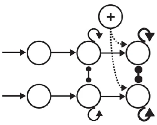
The Processing Stages of Decision Making. In the preceding section, we mentioned that a perceptual decision could not be formed with less than two stages: one stage for encoding the stimulus information and one stage for computing the decision variable from the first stage (Graham, 1989); But a more elaborate way to categorize the successive processing stages of decisions is depicted below:
From left to right:
1. The first stage is the evidence-encoding stage, comprised of groups of target-responsive or distractor-target-responsive populations of neurons (Target and distractor stimuli are specified with letters T and D in the picture above, respectively). Weak recurrent dynamics prevail on this level, which means the effective time constant is governed by leakage (leakage regime), which is far shorter than the time constant required to support evidence integration.
2. The integration of encoded evidence by integrator neural populations occurs at the second stage: there exist moderate to strong dynamics (recurrent excitatory connectivities and inhibition between populations), which set the stage to support the integration of encoded evidence projected from the first stage. Moreover, to control the strength of the dynamics means controlling the SAT (decision regime).
3. The last stage is the choosing stage that has very strong dynamics (shown by thick connectivities), which has a short effective time constant (little support for evidence integration) to an input with a critical level in the winner-take-all fashion; also called thresholding circuitry (Simen, 2012).
These three stages composed of neuron populations with different dynamics embody the different phases of bounded rationalization in representational (algorithmic) level, which are: 1. to acquire pieces of evidence, 2. to integrate the pieces of evidence, and 3. finally, to commit to a choice (Standage et al., 2014).
Hypotheses on Modeling SAT at the Implementation Level.
In light of the three stages described above, it is time to advance to the hypotheses describing the speed-accuracy trade-off, as one salient feature of the perceptual decision-making process.
There are three classes of hypotheses on the implementation of the SAT, depending on which stage out of three is being modulated (Standage et al., 2014). There exist revealing electrophysiological data (Heitz & Schall, 2012) supporting the occurrence of all three classes
of hypotheses, which merely demonstrate that these hypotheses are not mutually exclusive (Standage et al., 2014).
Modulation of the encoding of evidence. Data from a study in 2012 show that the baseline rates of visual neurons regardless of being target-in or target-out were higher under speed and lower under accuracy conditions before the onset of the stimulus (Heitz & Schall, 2012). The hypothesis suggests that, under the speed condition, all visual neurons receive a spatially non-selective common excitatory cognitive signal that increases their baseline activity. The increase in the baseline rate is equivalent to having a lower decision threshold, and consequently, accuracy conditions call for a weaker common signal; such a mechanism is referred to as gain modulation in attractor models.
Figure01-5: Modulation of the encoding of the evidence (Standage et al., 2014) Modulation of the Integration of Evidence, Encoded by the Previous Stage This class of hypotheses has three sub-classes: 1. Modulation of the rate of integration, 2. Modulation of the onset of integration, and 3. Modulation of the sensitivity of the integration circuits.
Evidence for the first sub-class abounds, demonstrating the change in the rate of rising in the integrators according to speed or accuracy conditions (Heitz & Schall, 2012).
There are also two hypotheses explaining the modulation of the rate of integration:
a) A spatially non-selective stationary excitatory cognitive signal applied to the integrators controls the strength of recurrent dynamics (gain modulation). Expectedly, stronger
and the opposite happens for the weaker signals (Furman & Wang, 2008; Roxin & Ledberg, 2008).
b) A time-dependent ramp signal (linearly increasing as time elapses) called the urgency signal applied to the integrators would control the ramp of the sigmoid gain function associated with the recurrent dynamics governing the support for integration and affecting the effective time constant (Standage et al., 2014).
Figure01-6: Modulation of the rate of integration of evidence (Standage et al., 2014)
The other subclass, modulation of the onset of integration, states that one inhibitory gate adjusts the onset of the integration which, as mentioned, equates adjusting the bound (Purcell, Hair, & Mills, 2012).
Figure01-7: Modulation of the onset of integration (Standage et al., 2014)
Finally, the last subclass of this category assumes that, depending on speed or accuracy condition, integrators select different sub-populations of evidence-encoding neurons (black and gray arrows representing two separate sets of encoded-evidence for two-speed and accuracy conditions) (Scolari, Byers, & Serences, 2012).
Figure01-8: Modulation of the Sensitivity to the Evidence (Standage et al., 2014) Modulation of the Amount of integrated evidence Adequate for Commitment to Choice. The hypotheses in this class are categorized into two subclasses, 1. Adjustment to the cognitive input added to the thresholding circuit input, and 2. Modulation of the connectivity strength between integrators and thresholding circuitry (Standage et al., 2014).
1. Modulation of non-selective input to thresholding circuitry: such a top-down, spatially non-selective signal does not have the same effective time constant adjustment
the dynamics in thresholding circuits are already strong; instead, if to commit to a choice entails a fixed level of activity from the previous stage (integrators), then the amount of the non-selective signal dictates how much of integrated evidence is required to make a decision. Under speed conditions, a higher level of the top-down signal allows for a faster but less accurate decision due to less available information (Forstmann et al., 2010; Frank, 2006; N. Green, Biele, & Heekeren, 2012; Simen, Cohen, & Holmes, 2006).
Figure 1-9: Modulation of the non-integrator signal into the thresholding circuitry (Standage et al., 2014)
2. Adjusting the strength of connectivity between integrators and thresholding populations, is a hypothesis proposed in a biophisacally-based model for saccadic decisions (Lo & Wang, 2006).
Figure 1-10: Connectivity Modulation between Integrators and Thresholding stage (Standage et al., 2014)