Science Arts & Métiers (SAM)
is an open access repository that collects the work of Arts et Métiers Institute of Technology researchers and makes it freely available over the web where possible.
This is an author-deposited version published in: https://sam.ensam.eu
Handle ID: .http://hdl.handle.net/10985/10920
To cite this version :
Guillaume VERMOT DES ROCHES, Gabriel REJDYCH, Etienne BALMES, Thierry
CHANCELIER - The Component Mode Tuning (CMT) method. A strategy adapted to the design of assemblies applied to industrial brake squeal In: Eurobrake, France, 201405 Eurobrake -2014
Any correspondence concerning this service should be sent to the repository Administrator : archiveouverte@ensam.eu
EB2014-SA-018
THE COMPONENT MODE TUNING (CMT) METHOD, A STRATEGY
ADAPTED TO THE DESIGN OF ASSEMBLIES APPLIED TO
INDUSTRIAL BRAKE SQUEAL
1,2Vermot des Roches Guillaume*, 3Rejdych Gabriel, 1,2Balmes Etienne, 3Chancellier Thierry 1SDTools, France, 2Arts et Metiers ParisTech, France, 3Chassis Brakes International, France
KEYWORDS – parametric reduction, structural dynamics, coupling, robust design, updating ABSTRACT - Numerical prototyping is widely used in industrial design processes, allowing optimization and limiting validation costs through experimental testing. Industrial
applications nowadays focus on the simulation of complex component assemblies that are generally mass produced. Coupling properties thus have to be modelled, updated and
accounted for variability. For squeal applications, simulations still fail at robustly producing exploitable results due to the systems complexity, while experimentations are limited for diagnostic and design improvement.
This paper presents a new application of the Component Mode Tuning, an efficient model reduction method adapted to quick system level reanalysis as function of component free modes, to study the effect of coupling. The impact of component coupling stiffness and coupling surface topology is thus assessed on a drum brake subassembly which design is sensitive to squeal. It is shown that significant system differences can come from coupling surface variations with patterns close to experimental observations. This emphases the need for refined analyses to control coupling in the perspective of robust modelling.
INTRODUCTION
Automotive brake design is nowadays oriented towards an optimized weight/performance ratio which tends to generate noisy systems. High friction coupling at dissipation interfaces is responsible for self-sustained instabilities that can yield high vibration levels in the auditive frequency range. The noise generated, known as squeal between 1 and 16 kHz, can attain 120dB in the vicinity of the wheel and constitute the main customer warranty cost in the brake domain. Robust design of silent brakes is thus a current stake for the industry.
The study of brake squeal has become over the years a very active field of research, experimentally and numerically (1) (2) (3) (4) (5) (6) (7). The recent increase in
computational power made possible the study of complex industrial numerical assemblies with the Finite Element (FE) method. Squeal simulations are however still not fully predictive and their exploitation for design remains an open question. The problem faced here indeed involves modelling of strong interface non-linearities at several scales in systems subjected to variability (mass-production, friction lining process …).
The aim of the present paper is to present an efficient simulation methodology based on the Component Mode Tuning (CMT) method (5), providing relevant design information regarding component participation in assemblies. This reduction method allows generating very compact models with exact nominal modes, thus allowing quick reanalysis studies at the system level as function of local properties variation. Its application here targets the system sensitivity to component mode and coupling variation.
The method is applied to a drum brake subassembly for which experiments could characterize differences between noisy and silent systems output from the same mass production process. This paper first presents the CMT framework, the reduction method and the introduction of component free modes as explicit Degrees Of Freedom (DOF). Then formalization for sensitivity analysis regarding component or coupling property variations is discussed. A second section presents the case of study and illustrates the direct analyses that can be
performed with the CMT. The third and last section illustrates the coupling sensitivity studies performed to assess the system variability regarding coupling properties.
1. THE CMT : A MODEL REDUCTION METHOD EXPLICITLY USING COMPONENT FREE MODES IN ASSEMBLIES
Reduction of components with a physical interface using assembled system modes Traditional Component Mode Synthesis (CMS) methods (8) (9) divide structures into components and make assumptions on their coupling properties. The most widespread technique is the Craig-Bampton method that explicitly uses component interface DOF to couple components reduced with no a priori system knowledge, as illustrated in figure 1left. Advances in eigenvalue solver optimization and computational power allows computing fully assembled nominal modes of very large structures. Development of new reduction methods for parametric design studies thus becomes possible.
Figure 1. Interface representation. Left: coupling by displacement (primal). Right: coupling by energy (dual).
The CMT method assumes that a physical coupling occurs between components. With disjoint interfaces, components have fully distinct DOF, as illustrated in figure 1right. One thus distinguishes component and coupling matrices, such that the dynamic stiffness of the assembly presented in figure 1 (no coupling between component 2 and 3), can be written
0 0 00 0 0 0 0 0 0 0 0 0 0 0 0 (1)
with the elastic stiffness of component i, the coupling stiffness block of coupling matrix I between components k and l.
The principle of the CMT method is to perform a blockwise reduction by defining a set of Rayleigh-Ritz vectors for each component i, so that the reduction basis T is written
0 0 00
0 0 (2)
In this formalism, no interface DOF is explicitly kept and the resulting model is very compact as its size is only related to the number of shapes retained for each component. The reduced dynamic stiffness can indeed be written
0 0 0 0 0 0 + 0 0 0 0 0 + 0 0 0 0 0 (3)
The idea is then to choose the restriction of the fully assembled system modes to each
component as Rayleigh-Ritz vectors, noted Φ|. In such case, the nominal reduced system will have exact modes. The system modes are trivially recovered from a linear combination of their restriction to each subdomain. Interfaces are thus reduced without altering system modes. A convergence study of the method can be found in (5).
Introduction of component modes in the reduction basis
In design specification phase, the impact of single component behaviour on the system response is of main interest. Component redesign for vibration is commonly controlled by frequency and shape variations. Such information is however difficult to recover as no trivial link exists between the behaviour of a free component and its coupled behaviour in a system. The idea of the CMT method is to analyse the participation of component free modes
(frequency and damping) in the assembly. Each component reduction basis can then be generated using the component i free/free modes , combined for accuracy with the trace of the exact system modes Φ| as explained in the previous section,
= Φ| (4)
In general the enhancement part Φ| does not verify the orthogonality conditions at the component level. One generates an orthonormal basis of the subspace generated by the combination of the chosen shapes. The component free/free modes are not modified by the orthonormalization process as their definition imply their orthogonality.
As a result of the orthonormalization process the reduced elastic stiffness is diagonal with the first terms corresponding to the square of the component free/free modes pulsations. The interface matrices are populated with full blocks corresponding to coupling components. Due to the reduction basis choice of equation (4), each retained component free/free mode participation in each assembled mode is directly related to an explicit DOF. Ranking of the reduced response DOF as function of magnitude thus provides a sorted and quantified list of component free/free mode participation in an assembled mode.
Sensitivity analysis for component modes and coupling properties
The exploitation of the CMT in this paper is based on the study of the system sensitivity to component modes and coupling. For a given model of mass and stiffness , the j-th real mode Φ of pulsation verifies
− !Φ = 0 (5)
which can be derived as function of a parameter p, writing
"#$#%− #&#% −#'() #% * Φ = − − ! #+( #% = − ( ) #+( #% (6)
Equation (6) does not always have a solution, as Z is singular to modal frequencies. It has solutions if and only if the left hand side is orthogonal to Z kernel, spanned by the real modes,
Φ !#+(
#% 0 (7)
The orthogonality condition (7) thus defines the sensitivity as the left multiplication of the left hand side of equation (6) by Φ and assuming that the real modes are mass normalized yields
#'()
#% Φ .#$#% #&#%/ Φ (8)
To study the sensitivity of the system frequencies to a component mode frequency with the CMT model, matrix #$
#% only has a single non null value on its diagonal at the line
corresponding to the desired component mode – its projection is then trivial.
Over sensitivity study, reanalysis of modifications to the system can be performed on the CMT model, with the following techniques,
• Variation of a component free/free mode frequency requires the modification of a single value in the elastic coupling stiffness.
• Linear variations of stiffness coupling can be performed by applying a proportionality coefficient to the desired reduced stiffness matrix defined in equation (3).
• Mass modification, and coupling stiffness distribution modify the matrices properties in a non-trivial way. The non-reduced matrix variation must then be projected on the reduction basis (2) for reanalysis. This however generally concerns very sparse matrices over a few components at a time so that the block topology of the reduction basis can be exploited to obtain computationally cheap generation.
The reanalysis itself being performed on very small models, computation time ranges in seconds and the parameter intervals can be refined to perform an easy tracking of frequency evolution as function of the parameters.
2. CMT ANALYSIS OF A DRUM BRAKE ASSEMBLY
Presentation of the drum plate assembly with cable guide and wheel cylinder
This paper application concerns a recent drum brake system that had a bad exploitation return for squeal, but only part of the production was noisy. Experimental Modal Analysis (EMA) was thus undertaken on several instances of the main brake subassembly, presented in figure 2, in an attempt to characterize the difference between noisy and silent configurations.
Figure 2. The brake drum subassembly (left), composed, of a plate, a wheel cylinder fixed with a single pin (middle), and a cable guide riveted over a backplate (right).
Two major coupling areas are present in this assembly, illustrated in figure 3, between the main plate and wheel cylinder, and the main plate and the cable guide. Coupling is nominally modelled as a series of Multiple Points Constraints (MPC) between component interfaces. To allow coupling tuning and the application of the CMT, the MPC have been relaxed by the introduction of a penalized coupling strategy at the same locations. It was found that using a
constant stiffness coupling of 107 N/mm did not alter the first 100 modes of the system or its
numerical conditioning in comparison to the initial MPC. For each coloured area of figure 3, a separated coupling stiffness is considered in correspondence to the formalism of equation (1). For the wheel cylinder, two main areas will be investigated, the planar surface (in red) and the cylindrical surface (in green).
Figure 3. The nominal coupling areas represented as multiple point constraints connections by coloured areas for the cable guide (left) and the wheel cylinder (right)
Comparisons between noisy and silent systems pointed out that most differences in the frequency range of interest were concentrated on non-rigid modes #7 and #8 (modes #13 and #14 if rigid body modes are counted). It was found in particular that mode #8 has significant frequency variations (7.5%) and shape variation (loss of MAC correlation) between noisy and silent configurations. This results are synthetized in figure 4left and 4middle.
Figure 4. Left: Frequency differences between a noisy and a silent system. Middle: recombined MAC between experimental configurations. Right: recombined MAC between the silent configuration and the nominal numerical model.
Numerical shapes can be well correlated to experimental shapes of the silent configuration, as presented in figure 4right. The numerical frequencies however are at 1600 Hz instead of 1400 Hz, which should be explained by the lack of component updating. Updating the topology of the drum plate and material properties is known to generate significant frequency variations. The objective being to illustrate the fact that refined parametric simulations can reproduce the same trends, no further experimental correlation will be discussed in this paper.
Figure 5 and 6 respectively present numerical modes #13 and #14 paired to experimental modes #7 and #8. It can be seen, that both modes show a movement of the wheel cylinder while only mode #14 shows a significant movement of the cable guide.
Figure 5. Simulation mode #13 at 1615Hz.
Noisy2allmodes Frequency Damping 435 0.08% 477 0.10% 860 0.14% 921 0.79% 1187 0.37% 1257 0.91% 1458 0.73% 1597 0.37% 1823 0.24% 1950 0.55% NoNoisy11 allmodes Frequency Damping 438 0.04% 482 0.16% 865 0.16% 926 0.24% 1172 0.50% 1244 0.66% 1416 2.02% 1495 0.22% 1825 0.24% 1937 0.90%
Figure 6. Simulation mode #14 at 1651 Hz. The right view provides a zoom in on the cable guide movement.
System analysis with the CMT
The CMT formalism presented in section 1 allows a direct analysis of component mode sensitivity of the assembly by the application of equation (8). Figure 7 presents a visualization of each system mode sensitivity to component free modes. The rivets, backplate, screw and pin are here omitted as no sensitivity was found for these components.
Figure 7. Assembled mode sensitivity to component modes (including rigid body modes). From left to right, sensitivity to the plate modes, the cable guide modes, the wheel cylinder modes. Dashed lines separate rigid body modes from flexible modes.
For such assembly, most modes are driven by the drum plate, as seen in figure 7left. At higher frequencies a spread effect can be observed as coupling induces significant modal interactions between components. Sensitivity to the cable guide modes is presented in figure 7middle. It has a local effect due the small number of modes involved in the frequency range of interest. The wheel cylinder is a very rigid component with its first flexible mode around 30 kHz. The system modes are thus only locally sensitive to its rigid body modes. What is captured in such sensitivity is that the system vibration induces a rigid movement of the wheel cylinder, the resulting frequency and shape is then function of the coupling area and the component mass. Figure 8 proposes an alternative view extracted from the results of figure 7 for specific assembly modes. Figure 8left shows a coupled mode between the plate and cable guide. The movement is mainly based on mode #10 of the plate and #8 of the cable guide.
Figure 8. Assembled modes #12, #13, #14 sensitivity to component modes (including rigid body modes).
Figure 8middle and 8right show the component mode sensitivity of system modes #13 and #14 that are under investigation, and which are only sensitive to their main backplate mode. Such result is non intuitive as mode #14, presented in figure 6 clearly shows a flexible
deformation of the cable guide. The cable guide flexion frequency has little effect on the system resulting frequency, but the potential contact openings at the tip of the link between the cable guide and its backplate seems to indicate that such mode can be sensitive to coupling.
3. COUPLING VARIATION ANALYSIS OF THE DRUM BRAKE
Choosing a relevant coupling modelling strategy remains nowadays an open question. In particular the coupling surface topology and the interface stiffness remain difficult to characterize experimentally and can be function of only partially controlled. This section presents how such parameters can be numerically handled to study their variations. System mode variation as function of a coupling stiffness parameter
Figure 9 presents a coupling analysis from the CMT model by distributing the relative
coupling strain energies as function of the coupling matrix for each system mode. Such study determines which interface is solicited for each system mode. It can for example be seen that the coupling between the rivet base and the drum plate (bkpriv*) is never solicited excepted for system rigid body modes.
Figure 9. Global coupling strain energy distribution for each assembled mode. Wheel cylinder coupling is concerned by (wcbscr, screw, wc2dru, wc2dru1, wcpin2). Cable guide coupling is concerned by (bkpftp, bkpftp1, ftpcgp, fptcgp1, rivcgp, rivcgp1, bkpriv, bkpriv1).
Cable guide coupling is spread between interactions with the rivet and backplate (ftpcgp*), and between the drum plate and backplate (bkpftp*). Wheel cylinder coupling shows little interactions, a few modes have significant planar and cylindrical coupling energy (wcd2dru*). For mode #13, a clear interaction with the wheel cylinder is found, as shown in figure 10, and mainly concerns the planar coupling part. The first idea is then to analyse the effect of the stiffness coupling parameter. Such analysis is direct as it suffices to apply a varying factor to some of the coupling stiffness matrices of the CMT model.
Figure 10. Left: Coupling strain energy distribution of modes #7 to #17 (including RBM). wc2dru is the planar coupling and wc2dru1 is the cylindrical coupling. Right: frequency evolution as the coupling stiffness parameter applied to wcbscr, screw, wc2dru, wc2dru1, wcpin2.
Reanalysis is performed very quickly, (0.5s instead of 1000s for each point). Figure 10right however shows that not significant frequency variation in the range of physically acceptable coupling stiffness could be observed.
For mode #14, a clear interaction between the cable guide and backplate and rivet is observed in figure 11. The coupling stiffness variation study however comes to the same conclusion. No impact could be found in physical coupling stiffness ranges for modes #13 and #14.
Figure 11. Left: Coupling strain energy distribution of modes #7 to #17 (including RBM). rivcgp* is the
coupling between rivet and cable guide, ftpcgp* is the coupling between the cable guide and intermediate plane, and bkpftp* is the coupling between the main plate and the intermediate plate. Right: frequency evolution as the coupling stiffness parameter applied to ftpcgp*, bkpftp*.
Sensitivity as function of the coupling spatial distribution
Although brutal coupling stiffness variation did not provide relevant solutions, it is well known that coupling surface topology can show significant variations (roughness effect, non-planarity…). It is thus proposed to study the effect of the coupling topology on the system frequencies and in particular modes #13 and #14.
Figure 12. Coupling topology area of variation. From left to right, wheel cylinder coupling area, progressive increase of the coupling area with a 1mm step from the left back corner, cable guide coupling area, progressive coupling area with a 1mm step from the rivets right side.
For the wheel cylinder coupling area, presented in figure 12left, the fixation is maintained by a screw at a specific place. A uniform coupling on the whole surface of potential contact is thus unlikely to happen. It is suggested to discretize this surface, starting from the screw vicinity to a linear extension with a step of 1mm (materialized in figure 12 by the different node mark colours), and generating 33 coupling configurations. The coupling stiffness
matrices here need to be assembled on the full model and projected on the CMT model, which takes a little longer to compute (30s) but is still much quicker than a full simulation (1000s).
Figure 13. Frequency evolution as function of the progressively increasing wheel cylinder coupling area. Left: global view from 0 to 3 kHz. Middle: zoom in on modes #12 to #14. Right: Recombined MAC evolution for modes #13 and #14 (non-rigid #7 and #8) compared to the nominal configuration.
As function of the stick length (extension of the wheel cylinder coupling area), a clear frequency variation occurs for some modes, in figure 13left. Mode #13 shows a significant evolution (yellow curve of figure 13middle). A 200Hz variation is observed with a clear separation of modes #13 and #14 frequencies. A recombined MAC tracking to the nominal configuration, also shows that mode #13 shape significantly evolves when the stick length diminishes, with little effect on mode #14 until very low values.
For the cable guide coupling area presented in figure 12right, the fixation is maintained by two rivets, on a non-perfectly planar surface (see figure 6). It is experimentally known that the horizontality of the cable guide is not well controlled, such that the coupling area may be increased to the cable guide tip. Using a 1mm step to the cable guide coupling tip, 7 coupling configurations can be tested, with the results presented in figure 14.
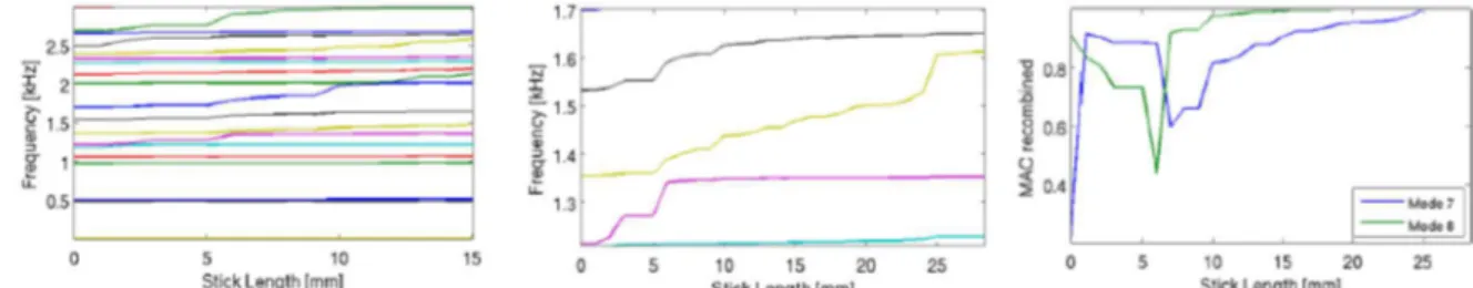
Figure 14. Frequency evolution as function of the progressively increasing cable guide coupling area. Left: global view from 0 to 3 kHz. Middle: zoom in on modes #12 to #14. Right: Recombined MAC evolution for modes #13 (non-rigid #7) and #14 (non-rigid #8) compared to the nominal configuration.
As function of the stick length, several modes show a frequency variation, seen in figure 14left. Figure 14middle shows that mode #14 has a 250Hz variation if the stick length is increased, with no effect on mode #13 frequency. The recombined MAC tracking to the nominal configuration also shows that mode shapes #13 and #14 are altered as function of the stick length with a specific length of 4mm where only mode shape #14 is altered.
Variation of the coupling surface topologies are thus capable of producing frequency and shape variations representative of what can be observed experimentally. Experimental correlation is however not perfect as the altered shapes obtained numerically did not show a better correlation to the noisy system. This may be due to the lack of component updating.
CONCLUSION
Numerical prototyping is nowadays widespread in the industry, but efficient exploitation for design remains a challenge for complex assemblies. Exploitable design rules must target component or coupling properties which are not directly linked to system level studies. The CMT framework presented in this paper allows making an explicit link between system modes and component free modes, so that each component mode participation in a system
mode can be analysed. The effect of component design variation on a system can then be quickly evaluated with an acceptable precision.
The effect of coupling in assemblies is most of the time not studied in details, although it is well known to have significant variation in mass produced systems. Studies adapted to the CMT strategy were here conducted regarding stiffness coupling coefficient and coupling surface topology variation. Although precise studies should involve non-linear tightening studies to obtain realistic stiffness distribution and topologies, basic studies can provide interesting variations and reproduce experimentally observed trends.
Component mode and coupling variation can be quickly reanalysed in the CMT framework with computations within seconds for nominal systems over 500,000 DOF. This permits refined parametric studies of the system local properties, allowing a proper mode tracking regarding frequency, shape and damping if necessary. Mode crossing patterns can also be analysed in details. Robust numerical design procedures can then become affordable. REFERENCES
(1) Fieldhouse, J. D., Newcomb, T. P., “Doubled pulsed holography used to investigate noisy brakes”, Optics and Lasers in Engineering, Volume 25 (6), pp. 455-494, 1996. (2) Giannini O., Akay, A, Massi, F, “Experimental analysis of brake squeal noise on a
laboratory brake setup”, Journal of Sound and Virbation, Volume 292 (1-2), 2006. (3) Ouyang, H., Nack, W., Yuan, Y., Chen, F., ”Numerical analysis of automotive disc
brake squeal: a review”, International Journal of Vehicle Noise and Vibration, 1, 3/4, pp. 207-231, 2005.
(4) Fritz, G, Sinou, J.-J., Duffal, M. and Jezequel, L. “Investigation of the relationship between damping and mode coupling patterns in case of brake squeal”, Journal of Sound and Vibration, Volume 307, pp.591-609, 2008.
(5) Vermot des Roches, G. “Frequency and time simulation of squeal instabilities.
Application to the design of industrial automotive brakes”, PhD thesis, Ecole Centrale Paris, CIFRE SDTools, 2010.
(6) Sinou, J.-J., Loyer, A., Chiello, O., Mogenier, G., Lorang, X. Cochetuex, F, Bellaj, S., “A global strategy based on experiments and simulations for squeal prediction on industrial railway brakes”, Journal of Sound and Vibration, Volume 331 (20), pp. 5068-5085, 2013
(7) Heussaff, A. Dubar, L. Tison, T., Watremez, M., Nunes, R. F., “A methodology for the modelling of the variability of brake lining surfaces”, Wear, Volume 289, pp. 145-149, 2012.
(8) Craig, R. Jr., “A review of Time-Domain and Frequency Domain Component Mode Synthesis Methods”, Int. J. Anal. and Exp. Modal Analysis, Volume 2, pp. 59-72, 1987.
(9) De Klerk, D., Rixen, D., Voormeeren, S. N., “General framework for dynamic substructuring: History, review and classification of techniques”, AIAA Journal, Volume 6 (5), pp. 1169-1181, 2008.