The Seasons of the True Size Anomaly
* Boris Fays1Georges Hübner2 Marie Lambert3 This draft: June 2020
Abstract
This paper employs a robust portfolio sorting procedure to factor size characteristics into returns. The US size anomaly boils then down to a pure seasonal effect, fully supporting the “tax-loss-selling” hypothesis. We build a long-short calendar trading strategy, easily reproducible by an asset manager, being long the Small-minus-Big (SMB) portfolio in January (or in Q1), staying in cash in Q2 and Q3, and shorting SMB in Q4. The strategy achieves a mean yearly return close to 11% from 1963 to 2019. It does not decay over time, remains steady across all subperiods, and resists to the detection of false discoveries.
Keywords: Size Premium, Fama-French Factors, DSN Factors, Calendar Anomaly, Turn-of-the-year Effect, January Effect.
* Marie Lambert and Georges Hübner acknowledge the financial support of Deloitte (Belgium and
Luxembourg). All remaining errors are ours.
1 Research Associate, University of Liège, HEC Liège, Belgium.
2 Corresponding author. Professor of Finance, University of Liège, HEC Liège, Belgium Tel: (+32) 4
2327428. E-mail: g.hubner@uliege.be. Mailing address: HEC Liège, 14 rue Louvrex, B-4000 Liège, Belgium.
Billions of dollars have been allocated to pure small-cap index funds since the size effect was initially discovered by Banz (1981). Nevertheless, the remuneration of the US size factor has considerably weakened over the last thirty years. The size factor has been predominantly measured as the excess return on a “small-minus-big” (SMB) portfolio constructed following the Fama and French (FF) (1993) guidelines1. Moreover, many papers have reported that these returns experience a sharp decline towards the end of the calendar year and then quickly recover during the first days of January (see Van Dijk (2011) for a complete review). However, a recent article on the CFA blog makes a “Case Against Small Caps” (CFA Blog)2 by showing that even when considering different ways to measure size in the US Stock Market or worldwide, it does not seem to be possible to boost its performance. In addition, the SMB portfolio returns of FF do not fully reveal the strong and steady seasonal pattern of the size premium. This might be because the underlying explanations of the calendar effect do not firmly hold or because the measurement issues with the FF premium do not allow us to identify the pattern. We believe that, despite all the efforts made thus far, the issue has not yet been fully addressed, not only regarding its existence but also whether it is, by nature, a reward for risk or a calendar anomaly.
In a methodological paper, Lambert et al. (2020) present an alternative methodology to FF (1993) with the aim of making the size and value premiums less prone to external and spurious influences, including their respective effects on each other. They call it the ‘dependent-symmetric-name’ (or, in short, DSN) procedure. Following their approach, we find evidence for the latter interpretation and exploit it through a seasonality-based trading strategy.
From an academic perspective, our research demonstrates that by measuring the size premium following this alternative method, we can identify a pure and strong seasonal pattern in the SMB portfolio return. In the next sections, we replicate the Lambert et al. (2020) procedure, apply it over a large time window, and unequivocally associate the size premium with the calendar effect. The behavior of the size premium indicates that the remuneration of the SMB portfolio only results from a seasonal effect and does not provide any additional reward for systematic risk: it exists, but as a market anomaly and not as a risk factor. Unlike most evidence published in the literature on alternative ways to measure the size premium, the calendar abnormal return evidenced in our paper does not decay or discontinue over time: the effect is alive and well, even at the moment of the writing of this paper. This is likely to result from the most convincing theoretical explanation of the effect, namely, the “tax-loss-selling” hypothesis for both individual and institutional investors. Its impact on stock returns is independent of market risk and will likely prevail as long as the U.S. tax system is not drastically reformed.
From a practical perspective, our results provide an opportunity for portfolio managers to exploit this calendar anomaly. We show that a mechanical trading strategy, by simply conditioning portfolio rebalancing on past and public information, can deliver abnormal returns over any period of time and would be exempt from any systematic risk. However, the effectiveness of this mechanical strategy hinges on how the SMB portfolio is constructed. An asset manager who uses the original FF portfolio compositions will not obtain satisfactory results. Rather, it is crucial for her to adopt the DSN procedure described in this paper. However, if she manages to replicate the composition of the DSN size
portfolio, the reward is worth the effort. Simply going long on the SMB portfolio in January (or in Q1), subsequently remaining in cash, and eventually shorting the SMB portfolio during the last quarter of the year achieves outstanding results for the whole 1963-2019 period. The average Sharpe ratio of this strategy exceeds 0.6 and remains very steady over time, with very few negative occurrences (as low as 2% of instances) on all possible rolling 5-year holding periods (613 in total). For portfolio managers who are not willing or allowed to adopt short positions, we show that a long-only strategy of buying small caps in Q1, then the market in Q2 to Q4 also achieves very satisfactory results. Nevertheless, since the Q4 effect only impacts small-cap stocks, the long-only strategy cannot exploit that part of the calendar anomaly.
1. Literature
The existence of seasonality in the size premium, known as the “turn-of-the-year effect”3
, has been widely documented in the literature since the initial study of Rozeff and
Kinney (1976). Nevertheless, the literature has long assumed that the size factor can survive the removal of this calendar effect because it reflects a reward for some source of risk inherent to small-capitalization stocks. In Table 1, we present a nonexhaustive list of academic references that debate the theoretical effects behind the size premium.
[Insert Table 1 here]
Overall, the seasonal behavior of the size premium bears two potential theoretical explanations: the “window-dressing” hypothesis and the “tax-loss-selling” hypothesis.4 The later hypothesis remains, however, a simple, robust and persistent tax-related distortion
in the behavior of large groups of investors to explain the seasonality of the size premium. The tax-loss-selling hypothesis not only explains the average monthly pattern of quintile portfolios sorted on firm size but also predicts a very strong persistence of the effect over time and independent of market conditions. 5 However, the current sets of findings (remuneration of a size factor and unstable seasonal effects) seem to cast doubt on the persistence of a steady January effect associated with small-cap stocks.
According to Ockham’s razor, before looking for sophisticated alternative explanations of the size effect, one should check whether this parsimonious type of explanation should not simply prevail. This motivates our investigation of a novel way of constructing the SMB portfolio.
2. The Factor Construction Method: Dependent, Symmetric Name
Breakpoints (DSN) Sort
For more than a quarter of a century, the mimicking portfolios for size and book-to-market risks developed by FF (1993), followed by the momentum factor of Carhart (1997), have firmly stood as the predominant standard in constructing fundamental risk factors. The authors consider two ways of partitioning U.S. stocks, i.e., a sort on market equity and a sort on book-to-market, and construct six value-weighted, two-dimensional portfolios at the intersections of the rankings.
We adopt the modified factor construction approach of Lambert et al. (2020) that jointly analyzes the three empirical risk dimensions (size, book-to-market, and momentum). This approach differs from the original FF methodology in three respects:
1. We replace the FF “independent” sort with a “dependent” sort, i.e., a multistage stock sorting procedure. Specifically, we successively perform three sorts. The first two sorts operate on “control risk” dimensions, followed by the risk dimension to be priced. We use the momentum effect documented by Jegadeesh and Titman (1993) and introduced in empirical asset pricing models by Carhart (1997) as the first control risk dimension6 and then use either the size or book-to-market as the second control, depending on whether one wants to isolate the book-to-market or size risk premium.
2. We adopt a symmetric sorting procedure: at each point in time, the full sample is divided into three portfolios of equal size. Then, every portfolio is itself split into three subportfolios of equal size. The last step finally partitions each of the nine subportfolios further in three parts to create a total of 27 equally weighted portfolios. 3. We perform a systematic and comprehensive sort on all listed stocks of the three U.S.
exchanges (NYSE-NASDAQ-AMEX), while FF only perform a heuristic split of the U.S. stocks according to the New York Stock Exchange (NYSE) as a reference point. These differing choices from FF underlie the so-called DSN procedure (a dependent sort that starts with the control variables and makes symmetric splits on the all-name sample breakpoints) to construct the size and value premiums. The aim of the DSN procedure is to detect whether, when controlling for two out of the three risk dimensions, there is still sufficient return variation related to the third risk criterion.
The DSN sorting produces 27 (3x3x3) portfolios capturing the return relating to a low, medium, or a high level of the risk factor, conditional on the levels registered on the two control risk dimensions. Taking the simple average of the differences between the
portfolios’ highest and lowest scores on the risk dimension to be priced while scoring at the same level for both control risk dimensions, we obtain the return variation related to the risk under consideration. To obtain the risk premium corresponding to dimension X, after sequentially controlling for dimensions Y and Z, the factor return can be computed as follows: 𝑋𝑌,𝑍,𝑡= 1 9[ ∑ ∑ 𝑅𝑡(𝐻𝑋|𝑏𝑌|𝑐𝑍) 𝑐=𝐻,𝑀,𝐿 𝑏=𝐻,𝑀,𝐿 − ∑ ∑ 𝑅𝑡(𝐿𝑋|𝑏𝑌|𝑐𝑍) 𝑐=𝐻,𝑀,𝐿 𝑏=𝐻,𝑀,𝐿 ] (1)
where 𝑅𝑡(𝑎𝑋|𝑏𝑌|𝑐𝑍) represents the return of a portfolio of stocks ranked a on dimension X, among the basket of stocks ranked b on dimension Y, themselves among the basket of stocks ranked c on dimension Z. Dimensions X, Y and Z stand for the factor to be priced and its control while H, M and L stand for high, medium and low, respectively. For instance, when dimension X corresponds to market cap, the premium is defined as low size (LX) minus high size (HX), or in short as SMB, as in FF.
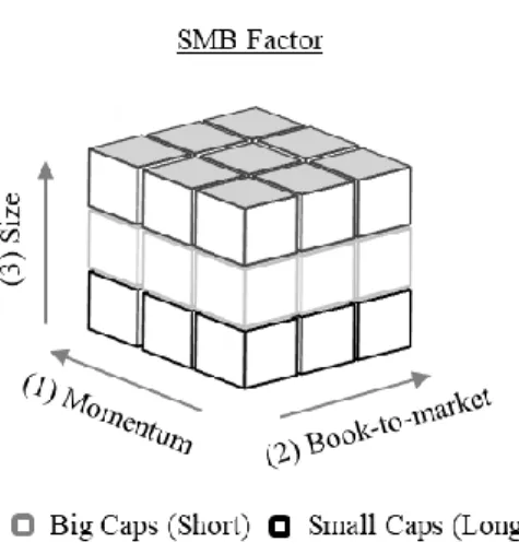
We illustrate the methodology with the construction of the SMB factor. We start by breaking up the NYSE, AMEX, and NASDAQ stocks universe into three groups according to the momentum criterion (first control). We then successively scale each of the three momentum portfolios into three classes according to their book-to-market fundamentals (second control). By splitting each of these nine portfolios once again to form three new subportfolios according to their market capitalization (variable to be priced), we end up with 27 value-weighted portfolios. The rebalancing is performed on an annual basis at the end of June of year y. An analogy could be made to a cubic construction, displayed in
Figure 1: each year, any stock integrates one slice, then one row, then one cell of a cube and thus enters one and only one portfolio. Among the 27 portfolios inferred from the DSN sorted risk factors, we retrieve only the 18 that score at a high or a low level on the risk dimension corresponding to the last sort performed, i.e., big-small. The nine self-financing portfolios are then created from the difference between high- and low-scored portfolios displaying the same ranking on the value and momentum dimensions (used as control variables). Each portfolio return is obtained as the value-weighted average of its components’ returns.7 Finally, the SMB risk factor is computed as the arithmetic average of these nine portfolios.
[Insert Figure 1 here]
3. Data
To construct the DSN portfolios and compare them with the FF portfolios, we use a single data set for both sets of factors. Our sample contains returns and accounting data for U.S. equities from the merger of the Center for Research in Security Prices (CRSP) tapes and Compustat data obtained from the XpressFeed Global database available on Wharton Research Data Services (WRDS). Our U.S. equity data include all available common stocks on the merged CRSP/Compustat data between July 1963 and July 2019.8 The stock selection criteria are as follows: a valid CRSP share code (SHRCD) of 10 or 11 at the beginning of month t, an exchange code (EXCHCD) of 1, 2 or 3 available shares (SHROUT) and price (PRC) data at the beginning of month t, available return (RET) data for month t, at least 2 years of listing on Compustat to avoid survival bias and a positive
book-equity value at the end of December of year y-1. We include delisting returns when available in the CRSP Event file.
We define the book value of equity as the Compustat book value of stockholders' equity (SEQ) plus the balance-sheet deferred taxes and investment tax credit (TXDITC). If available, we decrease this amount by the book value of the preferred stock (PSTK). If the book value of stockholders' equity (SEQ) plus the balance-sheet deferred taxes and investment tax credit (TXDITC) is not available, we use the firm's total assets (AT) minus its total liabilities (LT).
Book-to-market equity (BTM) is the ratio of the book value of equity for the fiscal year ending in the calendar year y-1 to market equity. Market equity is defined as the price (PRC) of the stock times the number of shares outstanding (SHROUT) at the end of June
y to construct the size characteristic and at the end of December of year y-1 to construct the
B/M ratio. Momentum is defined as in Carhart (1997), i.e., based on a t-2 until t-12 cumulative prior monthly return.
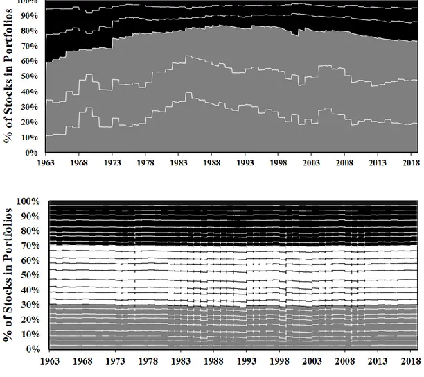
The DSN procedure corrects a major drawback of the FF factor construction method. By taking the intersection of two alternative partitions of the universe of stocks, the FF method does not ensure that each portfolio features an equal number of stocks. This may lead to some highly concentrated portfolios whose lack of diversification could alter their risk-return tradeoff. The DSN approach, through its sequential portfolio construction rules, guarantees the same number of stocks in all portfolios. In our sample, Figure 2 shows the impact of the difference between the two construction approaches throughout the years.
The upper graph shows that the FF procedure results in large time variations in the number of stocks and sometimes a very high concentration in the big portfolio, especially during the 1980s and 1990s. From a mean-variance efficiency perspective, this creates a disadvantage vis-à-vis the small portfolio regarding the diversification effect. By contrast, the DSN method ensures a constant proportion of stocks in each portfolio. Even though the midcap layer (in white on the graph) is discarded, each leg of the SMB portfolio has a reasonable and equal number of constituents at any time. Furthermore, by taking the arithmetic mean of nine portfolio returns, the small and big portfolios benefit from an additional averaging effect that reduces the potential impact of specific risk in each subportfolio.
4. Results
4.1. The Diverging Statistical Properties of the FF and DSN
Portfolios
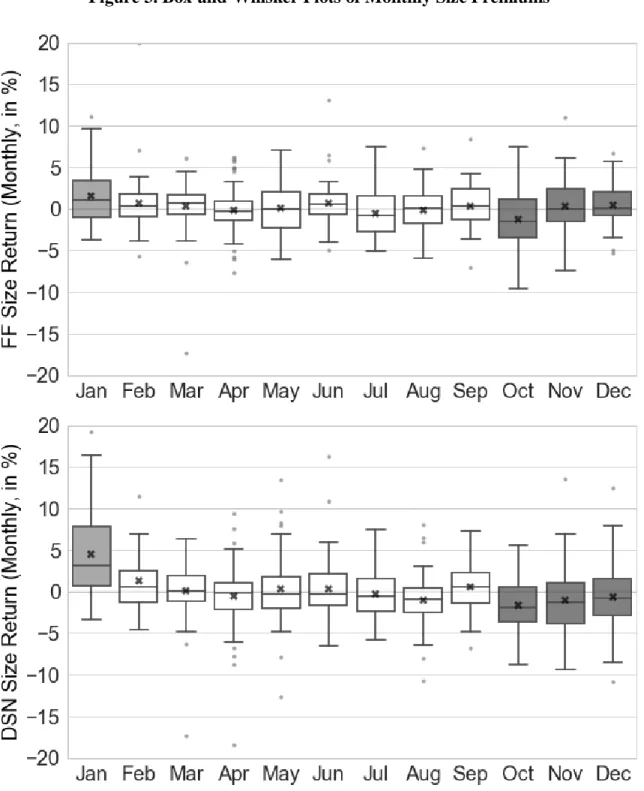
The inspection of the month-by-month behavior of the size factors over time reveals their seasonality. In Figure 3, we show the box-and-whisker plot of the FF and DSN monthly hedge portfolio returns. As already documented previously, the January return is generally higher than that of every other month. For the FF premiums, the lowest monthly return is observed in October, but the dispersion is very large. In the DSN graph, the pattern becomes much more contrasting: the distribution of the January returns tilts towards very positive values, whereas all three months of the last quarter have negative means and medians, and they also show the lowest first quartile in the sample.
The pronounced seasonality of the DSN size factor is a very distinctive property of the monthly, and even quarterly, distribution of returns. Calendar effects mostly appear around the turn of the year. To check their properties, we distinguish four periods: the month of January (Jan), the rest of the year (Feb.-Dec.), i.e., the eleven months from January to December, the first quarter (Q1), and the last quarter (Q4). The summary statistics of the FF and the DSN premiums are displayed in Table 2.
[Insert Table 2 here]
The results not only lend strong support to the visual impressions arising from the inspection of Figure 3 but also reveal other very insightful seasonal properties of the hedge portfolios.
The January effect. First, the January premium is especially strong under the DSN method: with a monthly mean return close to 5% (4.54% exactly), it translates into a very unusual annualized mean greater than 54%, without any negative outlier in more than half a century. The beta is almost nil, and the Sharpe ratio almost reaches a “Madoff-like” value of 3. The only downside of these outstanding statistics is the erosion rate of 59.94 basis points. This means that the excess return decreases by 5.0 bps in January every year. Over the 56 years of the sample period, this results in a reduction of 2.8% of the premium due to time decay. Thanks to the high volatility of the premium, this is not statistically significant but might be a source of concern when one wants to implement a longstanding calendar strategy.
Second, although the seasonal effect is also present in the FF January size premium, its statistical features are much less appealing. The SMB portfolio yielded an average of
1.61% in January every year, but the negative trending effect also eroded it by 7.6 bps every year: in total, the cumulative erosion factor totaled 7.6 bps x 56 years = 4.26%. This effect is highly significant and confirms the gradual disappearance of the January size effect emphasized in the literature (Medhian and Perry, 2002).
The rest-of-the-year effect. The rest-of-the-year (from February to December) size effect is very small and steady in the FF world. It is negative under the DSN method. Taking the beta into account, the SMB portfolio delivers a strongly negative and significant alpha. The first-quarter (Q1) effect. The first-quarter statistics show much weaker results than when considering the January effect alone. The FF size premium alpha, while still positive, becomes insignificant. The DSN premium remains high, but its alpha also sharply decreases. Overall, the January effect does not extend to February and March, but the DSN Sharpe ratio remains relatively high with a decay factor (32 bps/year) nearly half that of January (60 bps/year).
The last-quarter (Q4) effect. The last quarter is particularly insightful regarding the DSN premiums. The clustering of negative returns displayed in Figure 4 results in a large negative return. When the positive beta of the premium is taken into account, the alpha turns out to be very negative and significant. This quarterly negative risk premium does not appear to erode over time. In addition, although the figures are not as impressive as the January effect, they have the advantage of covering one quarter every year. For instance, considering the alpha, its value for January is 50.34%/12 = 4.19% per year. For the last quarter, it is equal to -21.40%/4 =-5.36% on average per year. Thus, shorting the SMB portfolio in fall is on average more profitable than being long this portfolio in January only.
Of course, nothing precludes the simultaneous adoption of a strategy of going long on the size portfolio in January and shorting it during the last quarter.
The analysis of this new strategy for the 1963-2019 period is conducted in the next section.
4.2. Taking Full Advantage of the Calendar Anomalies
We adopt the perspective of an equity market-neutral asset manager. For both the FF and the DSN hedge portfolio construction methods, our aim is to implement a simple long/short (L/S) size-calendar portfolio strategy to exploit the size premium and leave the beta low or close to zero. Since we work in-sample over the full time window of 56 years, such a strategy should not condition the investment decisions on any statistical estimate retrieved from the sample but rather on simple heuristic rules based on the suspicion of a stable seasonal pattern. Therefore, for each of the SMB portfolio construction methods, we test four simple rebalancing strategies that are represented in Table 3.
[Insert Table 3 here]
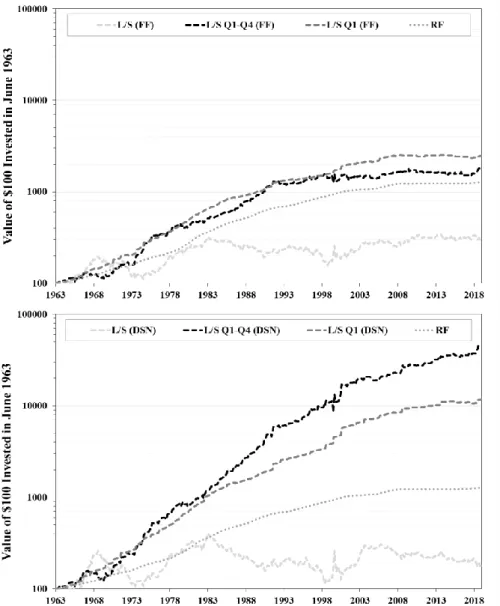
The results of the implementation of the L/S size-calendar strategies are represented in Figure 4. The logarithmic scale enables visualization of how steady the CAGR of the portfolios remains. As the portfolios are meant to remain market neutral, their minimal target should be the thin dotted line representing the risk-free investment over time. It is clear from the upper graph that the implementation of a calendar strategy with the FF size portfolios does not produce notable results. The January effect was effective during the seventies, but since then, the cumulative return of the L/S portfolios has evolved, at best,
in parallel to the riskless investment curve. Since the beginning of this century, shorting the size portfolio in Q4 (the continuous lines) would have destroyed value. The uselessness of attempting to time the size premium in the last quarter of the year probably explains why there has never been any real interest in this type of strategy in the literature. Since the FF size premium does not reveal any “fall” (Q4) effect, no one should truly care about it when implementing portfolio strategies.
[Insert Figure 4 here]
The lower graph of Figure 4 shows a drastically different picture. The January (or Q1) effect persists quite well over time, although the erosion of this calendar effect is observable in the recent period. However, if an investor combines a long position at the beginning of the year with a short one at year-end, the results become truly impressive as the exponential behavior of the curve persists over time. The gap with the riskless investment continually deepens, especially when the investor considers quarterly portfolio rebalancing: long SMB in Q1, remain neutral in Q2-Q3, and short it in Q4. The terminal value of an investment of $100 made in July 1963 would have yielded $45,056 in June 2019 (fifty-six years later). This represents a compound rate of return of 11.53% per year.
To further verify the properties of the long/short size-calendar strategies, we report in Table 4 the summary statistics of the eight portfolios tested above.
[Insert Table 4 here]
Although their mean excess returns and alphas are positive, the results for the strategies based on the FF factors support the observations drawn from Figure 4. Regarding the strategies based on the DSN premiums, thanks to the low beta of the SMB portfolio and
the long periods of no investment, the beta of all strategies is almost nil and totally insignificant: we can safely discuss equity market-neutral strategies. Thus, their alpha is almost equal to their mean excess return. The Sharpe ratios are all above 0.5, and the time trends are relatively close to zero, especially for the two strategies that involve shorting the size premium in Q4. However, there is one downside: with the exception of the pure January strategy, the minimum return is quite low. The long leg was reached in March 2000. This corresponds to the burst of the dot-com bubble, after its peak in February 2000, which hit small-cap stocks very hard. The short leg occurred in November 1999, before the peak of the same bubble. Note that during the highly volatile semester encompassing Q4-1999 and Q1-2000, three of the four size-calendar strategies remained profitable: +18.45% for L/S Jan, +33.85% for L/S Q1 and +6.61% for L/S Q1-Q4. Only strategy L/S Jan-Q4 delivered -8.79%. Thus, the low minima of the strategies are not particularly serious when considered in their broader context.
4.3. Does it Also Pay to be Long-Only?
Many asset managers could retort that their ability to benefit from the calendar anomaly would remain very limited. The hindrance lies in their long-only constraint. As the SMB portfolio means “small-minus-big”, being long or short, this hedge portfolio must involve shorting one of its legs, which is a luxury that asset managers cannot afford. Therefore, it is worth considering alternative strategies that allow the manager to be directionally exposed to the stock market at all times.
Being long, the small size portfolio means, in this context, making an equally weighted allocation to the 9 subportfolios represented in the bottom of the second cube in Figure 1.
That is, for all momentum terciles (left horizontal axis), then all book-to-market terciles (right horizontal axis), take the nine portfolios corresponding to the first size tercile (vertical axis). The same principle holds for an investment in the big portfolio but now focuses on the rear side of the same cube. When the portfolio is invested in neither the small- nor the large-cap DSN portfolio, we track the market.9 The outcome of the long-only strategies is presented in Table 5.
[Insert Table 5 here]
The benchmark of the long-only size-calendar portfolio is the market portfolio whose compound rate of return is 10.25% over the whole period. Moreover, the most profitable strategy would have been to invest in Q1 in the small portfolio, then track the market for the remaining 9 months. An investment of $1 in 1963 would have resulted in a final amount of $8,822, which is more than three times the market return, with a compound return of 17.61% per year. The table confirms that when one is constrained to remain long-only, switching from the market to the big portfolio in Q4 is useless. The highest alphas and Sharpe ratios are reached when the investor merely swaps the market for small caps in January or, even better, throughout the first quarter. As the graph clearly shows, remaining invested in small caps during the remaining three quarters destroys value. Finally, the time trends of all four strategies are positive but insignificant: there is no evidence that the Q1 small-cap effect vanishes over time.
Thus, the results for the long-only size-calendar strategies confirm the outcome of their long/short counterparts regarding the seasonal anomaly of small caps in Q1. Nevertheless, the failure to achieve equally good results by going long on large-cap portfolios in Q4
reveals that the end-of-year effect emphasized in the L/S analysis is largely due to a negative small-cap effect rather than a positive one on large caps. The whole quarterly seasonality that we have emphasized (SMB excess return is positive in Q1, negative in Q4) is attributable to the cyclicality of the small-capitalization stock returns, provided that these small-cap stocks are identified using the DSN procedure, not the original FF procedure.
5. Robustness test: The Persistence of Seasonality over Shorter Periods
No (or very few) investors have a horizon that encompasses the sample period of 56 years. In reality, not only do asset managers and their clients have shorter investment horizons, but they also enter and exit the market at different points in time. From a practical perspective, the whole analysis of the size-calendar strategies that we have performed thus far is of limited use if we do not take into account these two types of realistic constraints.
5.1. Considering subperiods
To reflect different financial cycles, we adapted the analysis to examine subperiods. If a calendar strategy truly exploits a market anomaly, it should resist various market conditions. Since we have a large sample time window at our disposal, we can split it in different ways to maximize the likelihood of observing different kinds of market cycles. In Table 6, we propose two partitions with different cycles: four windows of 14 years (the pivots are 1977, 1991 and 2005) and seven windows of 8 years (the pivots are 1971, 1979, 1987, 1995, 2003 and 2011).10 Table 6 reports the annualized mean return and Sharpe ratios of the four long/short size-calendar strategies with the DSN premiums along with the market portfolio for comparison purposes.
The series of mean returns clearly show a decreasing trend over time. This pattern logically follows from the strategies’ neutral investment in the riskless asset, whose evolution had been steadily decreasing since the 1980s. The pure January or Q1 strategies suffer the most from the post-2008 period, since they invest during 11 and 9 months per year in Treasury securities, respectively.
Despite the recent low interest rate environment, the L/S Jan-Q4 strategy posts an average yearly return that exceeds 5% for all subperiods, without exception. Except for the very first period of 8 years (1963-1971), this strategy can always provide a Sharpe ratio above 0.50. When a very long period of 14 years is considered, the Sharpe ratio of the L/S Jan-Q4 strategy is very stable, ranging from 0.60 to 0.86, always exceeding the market. By comparison, for the same subperiods, the Sharpe ratio of the global stock market ranges from 0.14 to 0.60.
Examining the most and least supportive stock market conditions is also insightful. The two most bullish subperiods were 07/1979-06/1987 (before the October crash) and 07/2011-06/2019. In both cases, the Sharpe ratio of the stock market exceeded one of the most profitable size-calendar strategies, namely, L/S Jan-Q4, by ca. 0.10, i.e., 10 basis points per unit of volatility. In contrast, during most bearish markets (07/1971-06/1979 and 07/2003-06/2011), while the stock exchange posted an average Sharpe ratio of 0.15, the same L/S Jan-Q4 strategy achieved an average of (1.15+0.72)/2 = 0.89, i.e., 0.01. six times the market’s reward-to-volatility ratio. The L/S Q1-Q4 strategy, slightly more profitable but also more volatile on average, shares a similar pattern and is even more countercyclical than the strategy of only going long on the SMB portfolio in January and shorting in Q4.
5.2. 5-year investment horizon
Our second adaptation of the global analysis is an examination of the profitability of the strategies in a sliding window environment. We adopt the perspective of an investor who wishes to stay invested for a medium horizon of 5 years but does not choose her entry and exit points. Thus, there are 613 possible verdicts of the portfolio management process, from June 1968 to June 2019. Focusing on the Sharpe ratio achieved by the “random entry” asset manager, we provide a summary of the results in Panel A of Table 7.
[Insert Table 7 here]
Once again, the best performing strategy is the L/S Jan-Q4. It delivers an average Sharpe ratio of 0.79. In approximately one third of cases, the Sharpe ratio exceeds 1.0 and is only negative in 2.1% of cases, namely, during 13 of the 613 periods considered. Once again, this strategy performs closely to but slightly better than L/S Q1-Q4.
The two strategies that both short the SMB portfolio in Q4 substantially outperform the strategies that focus on January or the first quarter only. However, this statement could be challenged from two perspectives: (i) the resilience of the outperformance to the ‘false discoveries’ phenomenon and (ii) the persistence of the outperformance over time.
(i) Resilience. The first way to challenge calendar-based trading strategies is to adopt a critical perspective on the testing of multiple portfolios. Starting from the series of 5-year Sharpe ratios, we can consider that our rolling strategy is equivalent to 60 consecutive situations in which the investor initially enters the market at a certain moment between July 1963 and June 1968, holds the strategy for 5 years, immediately starts over again for a new period of 5 years, and so on until the end of the time window. For each situation, we have
11 or 10 nonoverlapping series of 5-year portfolio returns11 that correspond to the different entry points and that, under the null hypothesis of no abnormal performance, correspond to a sequence of multiple strategies.12 The simplest approach to evaluate the performance of these strategies is to use the Student t-test. However, Harvey and Liu (2014) criticize this approach when testing multiple strategies because one of them will mechanically exhibit the best statistical performance simply because of chance. This is the phenomenon of “false discoveries” emphasized by Barras et al. (2010). To limit the issue of Type I error (rejecting the null hypothesis when it is true), they suggest two kinds of approaches: the familywise error rate (FWER) and the false discovery rate (FDR) families of tests, but they differ in their severity. The FWER deems it unacceptable to make a single false discovery, while the FDR accepts a certain fraction of mistaken rejections of the null hypothesis.
When 𝐾 strategies are tested and their associated p-values are ranked from the best (lowest) one with index 𝑘 = 1 to the worst (highest) one with index 𝑘 = 𝐾, the easiest FWER approach is the Holm criterion:
FWER: 𝑅𝐻0 if 𝑝𝑘 < 𝛼
𝐾+1−𝑘 (2)
where 𝛼 is the critical significance level. Regarding the FDR approach, we adopt the following rejection criterion:
FDR: 𝑅𝐻0 if 𝑝𝑘 < (𝐾+1−𝑘)𝛼 𝐾 ∑ 1 𝑖 𝐾 𝑖=1 (3)
In Panel B of Table 7, we show the proportions of series of DSN long/short portfolio returns with Sharpe ratios that significantly differ from zero and from 0.40. The latter figure is more relevant for the assessment of outperformance, as it corresponds to the average
Sharpe ratio of the market portfolio throughout the period. The first two calendar strategies fail to deliver convincing levels of outperformance. The strict FWER test diagnoses that the January calendar strategy never reaches any significant Sharpe ratio, and the figures are hardly better for the L/S Q1 strategies. Although the L/S Jan-Q4 strategy achieves better figures historically, it appears that it does not dominate the L/S Q1-Q4 strategy in terms of significance. In particular, when the investor is very demanding regarding outperformance and wishes to ensure that her strategy is able to beat the market (with Sharpe ratio greater than 0.4) without any hesitation (with the FWER test), she can be confident that this will happen more than 10% of the time. This means that, starting the strategies in the 1960s and ending 56 years later, the L/S Q1-Q4 calendar strategy will surely beat the market once.
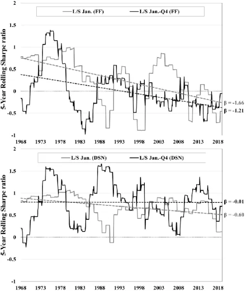
(ii) Persistence. Regarding the persistence of the strategies’ performance, the DSN portfolios that short the SMB portfolio in Q4 are also noteworthy. Figure 5 contrasts the 5-year rolling Sharpe ratios of the two January-based L/S size-calendar strategies for the premiums generated with the FF and DSN procedures.
[Insert Figure 5 here]
The decaying tendency of the calendar strategies with the original FF premiums is clearly visible in the upper graph. The trend is especially clear for the Jan-Q4 strategy after 1987. The lower graph shows that the January-only strategy with the DSN size factor almost always delivers positive and even comfortable Sharpe ratios, with two exceptions: the 1980-1992 period (looking 5 years back for the computation of the ratios), which corresponds to the inception of the decreasing interest rate trend, and the 2015-2019 period, which again corresponds to a downside rally on the interest rate market. For the L/S
Jan-Q4 strategy, the trajectory appears to be more cyclical but without trend and with oscillations that typically range from above 0.0 to above 1.0, with a long-run average of 0.79, as shown in Panel A of Table 7.
Overall, the acid test of different investment horizons and entry points does not disprove the favorable diagnosis of a simple calendar strategy applied to the SMB portfolio, provided that this portfolio is designed using the DSN procedure. Clearly, the addition of shorting this portfolio during the last quarter of each year brings additional value. More important, the phenomenon does not seem to fade away over time, and even an investor with a limited investment horizon is very likely to reap the calendar premium at many points in time, and even almost surely at one point in time as it were a pure unnoticed anomaly.
5.3. Transaction costs
The transaction costs associated with the liquidity of small caps might be another concern for the L/S strategies presented in this study. To account for transaction costs, we use the methodology from Hasbrouck (2009), who develops individual stock estimates from Gibbs sampling. When the estimate is missing for one stock, we follow the approach of Novy-Marx and Velikov (2016) and interpolate this estimate with the valid estimate of the stock, which possesses - at the same date - the closest Euclidean distance between size and idiosyncratic volatility to the stock with a missing estimate. Each time a position is entered into or exited, we assume that half of the effective bid-ask spread is paid, as in Chen and Velikov (2018).
Table 8 reports the performance of the L/S strategies net of estimated transaction costs. Despite that the strategies present, by design, high turnover (i.e., turning over the long and short legs of the SMB factor at least twice a year), the abnormal return (αCAPM) of all strategies remains positive and significant with, at least, a 95% confidence level. Any mitigation techniques similar to that found in Novy-Marx and Velikov (2016) might thus help to fully exploit the intrinsic qualities of the size-based seasonal strategies that combine information on the first and the last quarters of the year.
6. Concluding Remarks
The first important takeaway of our paper refers to the debate over the interpretation of the size premium and its practical importance: is it a risk factor, a calendar effect, or neither? This debate has certainly been fueled by the imperfections surrounding the construction of the benchmark in this field, namely, the FF small-minus-big portfolio. By adapting their methodology with a dependent, symmetric and full name-breakpoint sorting procedure (the so-called DSN approach of Lambert et al. (2020)), we provide a clear and unambiguous answer that has potential far-reaching implications for informational market efficiency and active portfolio management: the “size” effect is, according to our findings, a pure and strong seasonal anomaly. It is consistently positive in January and negative during the last quarter of the year, and this is true for more than half a century. Beyond that effect, we find no remuneration for size risk. This result, combined with the absence of specific remuneration for large-cap stocks during the last quarter of the year, lends strong support to the “tax-loss-selling” selling hypothesis that explains the small-cap effect through the tax-driven trades of institutional and individual investors around year-end.
With such an explicit answer to the size premium debate, we have adopted the practical perspective of an asset manager who applies a consistent trading strategy. The outcome accords with our expectations. We managed to create a very simple portfolio rebalancing rule, with long/short trades on value-weighted stock allocations, whose results confirm the claim made above, even when using different investment horizons and entry points. More important, the phenomenon does not seem to fade away over time, and even an investor with a limited investment horizon is very likely to reap the calendar premium at many
points in time, and even almost surely at one point in time as if it were a pure unnoticed anomaly.
Naturally, professional asset managers may retort that this still represents a desktop exercise, and the practical implementation of the strategies presented in this paper could severely weaken its actual results. We do not believe that the potential trading limitations of the calendar strategy are too restrictive, as we show that the strategies are still viable after accounting for estimated transaction costs even without applying any cost mitigation technique. Additionally, the long/short size-calendar strategy builds on past and public information and only induces portfolio rebalancing once per month, and its adoption of value-weighted portfolios mitigates the “microcap” issue already emphasized in the literature. Furthermore, the strategy does not come out of the blue: it is a natural consequence of simple, widely documented, and very rational tax-related investment behavior. All that is needed was to find the right way of measuring the size effect – this is the merit of the DSN approach that we applied in this paper.
7. References
Arnott, Robert D., Jason Hsu, and Philip Moore. 2005. “Fundamental Indexation.”
Financial Analysts Journal 61 (2): 83–99.
Asness, Clifford S., Andrea Frazzini, Ronen Israel, Tobias J. Moskowitz, and Lasse H. Pedersen. 2018. “Size Matters, If You Control Your Junk.” Journal of Financial
Economics 129 (3) 479–509.
Banz, Rolf W. 1981. “The Relationship between Return and Market Value of Common Stocks.” Journal of Financial Economics 9 (1): 3–18.
Barras, Laurent, Olivier Scaillet, and Russ Wermers. 2010. “False Discoveries in Mutual Fund Performance: Measuring Luck in Estimated Alphas.” Journal of Finance 65 (1): 179–216.
Berk, Jonathan B., Richard C. Green, and Vasant Naik. 1999. “Optimal Investment, Growth Options, and Security Returns.” Journal of Finance 54 (5): 1553–1607. https://doi.org/10.1111/0022-1082.00161.
Carhart, Mark M. 1997. “On Persistence in Mutual Fund Performance.” Journal of Finance 52 (1): 57–82. https://doi.org/10.2307/2329556.
Chen, Andrew Y., and Mihail Velikov. 2018. “Accounting for the Anomaly Zoo: A Trading Cost Perspective.” Working Paper. https://doi.org/10.2139/ssrn.3073681. Daniel, Kent, Sheridan Titman, and K. C. John Wei. 2001. “Explaining the Cross-Section
of Stock Returns in Japan: Factors or Characteristics?” Journal of Finance 56 (2): 743–66. https://doi.org/10.1111/0022-1082.00344.
Easterday, Kathryn E., Pradyot K. Sen, and Jens A. Stephan. 2009. “The Persistence of the Small Firm/January Effect: Is It Consistent with Investors’ Learning and Arbitrage Efforts?” Quarterly Review of Economics and Finance 49 (3): 1172–93. https://doi.org/10.1016/j.qref.2008.07.001.
Fama, Eugene F., and Kenneth R. French. 1993. “Common Risk Factors in the Returns Stocks and Bonds.” Journal of Financial Economics 33 (1): 3–56. https://doi.org/10.1016/0304-405X(93)90023-5.
Grinblatt, Mark, and Tobias J. Moskowitz. 2004. “Predicting Stock Price Movements from Past Returns: The Role of Consistency and Tax-Loss Selling.” Journal of Financial
Economics 71 (3): 541–79. https://doi.org/10.1016/S0304-405X(03)00176-4.
Gu, Anthony Yanxiang. 2003. “The Declining January Effect: Evidences from the U.S. Equity Markets.” Quarterly Review of Economics and Finance 43 (2): 395–404. https://doi.org/10.1016/S1062-9769(02)00160-6.
Harvey, Campbell R., and Yan Liu. 2014. “Evaluating Trading Strategies.” Journal of
Portfolio Management 40 (5): 108–18. https://doi.org/10.3905/jpm.2014.40.5.108.
———. 2019. “Lucky Factors.” Working Paper. https://doi.org/10.2139/ssrn.2528780. Hasbrouck, Joel. 2009. “Trading Costs and Returns for U. S. Equities: Estimating Effective
Costs from Daily Data.” Journal of Finance 64 (3): 1445–77. https://doi.org/10.1111/j.1540-6261.2009.01469.x.
He, Jia, Lilian Ng, Qinghai Wang, Lilian Ng, and Qinghai Wang. 2004. “Quarterly Trading Patterns of Financial Institutions.” The Journal of Business 77 (3): 493–509.
Jegadeesh, Narasimhan, and Sheridan Titman. 1993. “Returns to Buying Winners and Selling Losers: Implications for Stock Market Efficiency.” Journal of Finance 48 (1): 65–91.
Keim, Donald B. 1983. “Size-Related Anomalies and Stock Return Seasonality: Further Empirical Evidence.” Journal of Financial Economics 12 (1): 13–32. https://doi.org/10.1016/0304-405X(83)90025-9.
Lakonishok, Josef, Andrei Shleifer, Richard Thaler, and Robert Vishny. 1991. “Window Dressing by Pension Fund Managers.” The American Economic Review 81 (2): 227– 31.
Lambert, Marie, Boris Fays, and Georges Hübner. 2020. “Factoring Characteristics into Returns: A Clinical Study on the SMB and HML Portfolio Construction Methods.”
The Journal of Banking and Finance 114, 105811.
https://doi.org/10.1016/j.jbankfin.2020.105811.
Mehdian, Seyed, and Mark J. Perry. 2002. “Anomalies in US Equity Markets: A Re-Examination of the January Effect.” Applied Financial Economics 12 (2): 141–45. https://doi.org/10.1080/09603100110088067.
Ng, Lilian, and Qinghai Wang. 2004. “Institutional Trading and the Turn-of-the-Year Effect.” Journal of Financial Economics 74 (2): 343–66. https://doi.org/10.1016/j.jfineco.2003.05.009.
Novy-Marx, Robert, and Mihail Velikov. 2016. “A Taxonomy of Anomalies and Their Trading Costs.” The Review of Financial Studies 29 (1): 104–47. https://doi.org/10.1093/rfs/hhv063.
Reinganum, Marc R. 1983. “The Anomalous Stock Market Behavior of Small Firms in January.” Journal of Financial Economics 12 (1): 89–104. https://doi.org/10.1016/0304-405X(83)90029-6.
Rozeff, Michael S., and William R. Kinney. 1976. “Capital Market Seasonality: The Case of Stock Returns.” Journal of Financial Economics 3 (4): 379–402. https://doi.org/10.1016/0304-405X(76)90028-3.
Sikes, Stephanie A. 2014. “The Turn-of-the-Year Effect and Tax-Loss-Selling by Institutional Investors.” Journal of Accounting and Economics 57 (1): 22–42. https://doi.org/10.1016/j.jacceco.2013.12.002.
Van Dijk, Mathijs A. 2011. “Is Size Dead? A Review of the Size Effect in Equity Returns.”
Journal of Banking and Finance 35 (12): 3263–74.
Vassalou, Maria, and Yuhang Xing. 2004. “Default Risk in Equity Returns.” The Journal
Table 1
Milestones in the Explanation of the Size Premium
Authors Journal13 Evidence on the size effect
Banz (1981) JFE The size effect, small stocks outperform large stocks, is distinct from the market beta.
Keim (1983) JFE The size effect is associated with the returns observed in January.
Reinganum (1983) JFE The seasonal behavior of the size premium relates to the “tax-loss-selling” hypothesis. Lakonishok et al. (1991) AER The seasonal behavior of the size premium relates to the “window-dressing” hypothesis. Fama and French (1993) JFE The size factor (SMB) is introduced in asset pricing
models.
Berk et al. (1999) JF The stock returns related to firm size are associated with real options.
Daniel et al. (2001) JF The size factor might be a proxy for the investors’ biases in decision making.
Gu (2003) QREF The size turn-of-the-year effect is volatile and tends to fade away over time.
Grinblatt and Moskowitz (2004) JFE Individual investors' behavior feed the “tax-loss-selling” hypothesis.
He et al. (2004) JB Institutional investors' behavior feeds the “window-dressing” hypothesis. Ng and Wang (2004) JFE The tax-based selling behavior extends to the whole last
quarter of the year.
Vassalou and Xing (2004) JF The size premium is associated with a default risk. Arnott et al. (2005) FAJ The size effect might arise from noise in stock prices due
to trading or microstructure.
Easterday et al. (2009) QREF An arbitrage portfolio based on the size effect might deliver insufficient wealth effect.
Van Dijk (2011) JBF The size premium as a source of systematic risk seems to contradict empirical evidence.
Sikes (2014) JAS Institutional investors' behavior also supports a global tax-related explanation for the seasonality of the size effect. Asness et al. (2018) JFE Controlling for corporate quality effects revives the size
Table 2
Summary Statistics of the Seasonal Size Premiums, July 1963-June 2019
Jan. - Dec. Jan. Feb. - Dec. Q1 Q4
SMBFF Mean (an.) 2.46% 19.38% 1.21% 10.63% -1.88% Std (an.) 10.40% 11.82% 10.81% 11.03% 10.58% Min -17.38% -3.66% -21.92% -9.13% -12.90% Max 20.01% 11.07% 27.35% 15.55% 13.04% Skew 0.43 0.76 0.15 0.2 0.42 Kurt 4.99 0.24 -0.08 -0.29 0.29 βCAPM 0.21** 0.17* 0.27** 0.25** 0.29** αCAPM -3.44%** 12.63%* -5.09%** 3.74% -9.93%** SR -0.2 1.26 -0.33 0.56 -0.62 Exc. Return Trend (an.) 0.20 bps -91.23 bps ** 9.92 bps -31.16 bps* 18.35 bps Obs. 672 56 55 56 56 SMBDSN Mean (an.) 1.99% 54.44% -1.88% 23.72% -12.79% Std (an.) 14.51% 17.06% 17.45% 14.66% 14.96% Min -18.37% -3.35% -34.33% -6.78% -23.20% Max 33.68% 19.26% 52.83% 28.52% 24.62% Skew 1.16 0.88 0.9 0.72 0.73 Kurt 8.2 0.61 1.64 0.43 2.87 βCAPM 0.04 -0.02 0.45** 0.19 0.34** αCAPM -2.86% 50.34%** -9.20%** 4.75%** -21.40%** SR -0.18 2.93 -0.38 1.32 -1.17 Exc. Return Trend (an.) -0.36 bps -59.94 bps -0.60 bps -32.19 bps 5.36 bps Obs. 672 56 55 56 56
Note: The abbreviation “FF” refers to the Fama-French (1993) sorting method, whereas the abbreviation “DSN” refers to the dependent, symmetric on all names breakpoint sorting method. * and ** indicate statistical significance at the 0.05 and 0.01 levels, respectively.
Table 3
Design of the Long/Short Size-Calendar Strategies
L/S Strategies Q1 Q2 - Q3 Q4
Jan. Feb. Mar. Apr.-Sep. Oct. Nov. Dec.
L/S only +SMB
L/S Jan +SMB +RF
L/S Q1 +SMB +RF
L/S Jan-Q4 +SMB +RF S
Table 4
Summary Statistics of the Long/Short Size-Calendar Strategies, July 1963-June 2019 L/S Jan L/S Q1 L/S Jan-Q4 L/S Q1-Q4 SMBFF Mean (an.) 5.81% 6.13% 5.13% 5.44% Std (an.) 3.69% 5.99% 6.37% 7.93% Min -3.66% -17.38% -10.95% -17.38% Max 11.07% 20.01% 11.07% 20.01% Skew 4.76 1.54 0.51 0.46 Kurt 37.94 46.06 8.75 15.96 βCAPM 0.02* 0.04** -0.05** -0.03 αCAPM 1.11%** 1.30% 0.86% 1.05% SR 0.34 0.26 0.09 0.11 Exc. Return Trend (an.) -0.63 bps ** -0.60 bps -0.53 bps -0.50 bps Obs. 672 672 672 672 SMBDSN Mean (an.) 8.73% 9.40% 10.88% 11.55% Std (an.) 6.36% 8.99% 9.07% 11.06% Min -3.35% -17.37% -13.59% -17.37% Max 19.26% 33.68% 19.26% 33.68% Skew 5.75 4.6 1.58 2.17 Kurt 39.6 50.88 11.44 22.06 βCAPM 0.01 0.01 0 0.01 αCAPM 4.11%** 4.74%** 6.31%** 6.94%** SR 0.64 0.53 0.68 0.62 Exc. Return Trend (an.) -0.41 bps -0.59 bps -0.03 bps -0.21 bps Obs. 672 672 672 672
Note: The abbreviation “FF” refers to the Fama-French (1993) sorting method, whereas the abbreviation “DSN” refers to the dependent, symmetric on all names breakpoint sorting method. * and ** indicate statistical significance at the 0.05 and 0.01 levels, respectively.
Table 5
Summary Statistics of the DSN Long-Only Size-Calendar Strategies, July 1963-June 2019
L-O Jan. L-O Q1 L-O Jan.-Q4 L-O Q1-Q4
Mean (an.) 16.21% 17.98% 15.58% 17.35% Std (an.) 17.22% 18.40% 17.47% 18.64% Min -22.64% -22.64% -23.64% -23.64% Max 29.04% 34.59% 29.04% 34.59% Skew 0.36 0.55 0.25 0.45 Kurt 3.88 4.97 4.01 4.98 βCAPM 1.02** 1.03** 1.03** 1.04** αCAPM 5.10%** 6.83%** 4.41%** 6.13%** SR 0.68 0.73 0.63 0.69 Exc. Return Trend (an.) 0.42 bps 0.09 bps 0.47 bps 0.14 bps Obs. 672 672 672 672
Note: The abbreviation “DSN” refers to the dependent, symmetric on all names breakpoint sorting method. * and ** indicate statistical significance at the 0.05 and 0.01 levels, respectively.
Table 6
Annualized Mean Monthly Return and Sharpe Ratios of the DSN Long/Short Size-Calendar Strategies, July 1963-June 2019
Partition: 4x14 years
Mean L/S Jan. L/S Q1 L/S Jan.-Q4 L/S Q1-Q4 Mkt 07/1963-06/1977 11.03% 12.19% 12.23% 13.39% 7.20% 07/1977-06/1991 10.57% 12.09% 13.98% 15.49% 15.18% 07/1991-06/2005 9.79% 9.65% 11.04% 10.89% 11.60% 07/2005-06/2019 3.54% 3.66% 6.28% 6.40% 9.87% Sharpe Ratio 07/1963-06/1977 0.85 0.81 0.73 0.75 0.14 07/1977-06/1991 0.59 0.69 0.82 0.91 0.42 07/1991-06/2005 0.70 0.44 0.60 0.44 0.54 07/2005-06/2019 0.52 0.47 0.86 0.80 0.60 Partition: 7x8 years
Mean L/S Jan. L/S Q1 L/S Jan.-Q4 L/S Q1-Q4 Mkt 07/1963-06/1971 9.74% 9.75% 8.16% 8.17% 9.00% 07/1971-06/1979 12.46% 15.49% 16.42% 19.44% 6.25% 07/1979-06/1987 11.92% 11.94% 12.85% 12.87% 19.21% 07/1987-06/1995 8.49% 9.57% 13.35% 14.43% 11.49% 07/1995-06/2003 11.05% 11.88% 14.36% 15.19% 10.12% 07/2003-06/2011 4.94% 4.15% 5.08% 4.30% 7.85% 07/2011-06/2019 2.54% 3.00% 5.96% 6.42% 12.82% Sharpe Ratio 07/1963-06/1971 0.81 0.63 0.36 0.32 0.33 07/1971-06/1979 0.89 1.07 1.15 1.31 0.02 07/1979-06/1987 0.59 0.44 0.52 0.45 0.63 07/1987-06/1995 0.53 0.62 0.91 0.97 0.41 07/1995-06/2003 0.72 0.46 0.72 0.56 0.33 07/2003-06/2011 0.65 0.40 0.52 0.35 0.39 07/2011-06/2019 0.45 0.49 0.90 0.92 0.98
Table 7
Statistics of 5-year Sharpe Ratios of the DSN Long/Short Size-Calendar Strategies, June 1968-June 2019
L/S Jan. L/S Q1 L/S Jan.-Q4 L/S Q1-Q4 Panel A: Descriptive Statistics
Mean 0.70 0.61 0.79 0.75 Std 0.25 0.33 0.45 0.52 Min -0.12 -0.22 -0.23 -0.14 Max 1.07 1.61 1.66 1.88 Pr(>1.0) 7.90% 8.40% 32.90% 27.80% Pr(<0.5) 14.70% 38.20% 29.40% 39.30% Pr(<0.0) 2.00% 3.80% 2.10% 6.00% Obs. 613 613 613 613
Panel B: Multiple Testing
𝑯𝟎: 𝑺𝑹 = 𝟎 Basic t-test 51.70% 31.80% 55.80% 44.20% FDR test 8.00% 11.30% 31.00% 26.40% FWER test 0.00% 4.10% 22.50% 21.70% 𝑯𝟎: 𝑺𝑹 = 𝟎. 𝟒 Basic t-test 0.00% 4.10% 23.00% 21.90% FDR test 0.00% 3.90% 13.50% 18.40% FWER test 0.00% 0.20% 3.30% 10.30%
Note: The abbreviation “DSN” refers to the dependent, symmetric on all names breakpoint sorting method. The significance of the Sharpe ratio tests in Panel B is based on a 5% one-tailed test.
Table 8
The DSN Long/Short Size-Calendar Strategies Net of Transaction Costs, June 1963-June 2019 L/S Jan. L/S Q1 L/S Jan.-Q4 L/S Q1-Q4 E[rgross] 8.73% 9.40% 10.88% 11.55% αCAPM 0.0411** 0.0474** 0.0631** 0.0694** TCs 2.12% 2.18% 3.57% 3.57% E[rnet] 6.61% 7.21% 7.32% 7.97% αCAPM 0.0214** 0.0269* 0.0281* 0.0336*
Note: As in Novy-Marx and Velikov (2016), the transaction costs are estimated using the Hasbrouck (2009) method, and TCs denote the average yearly transaction costs over the sample period. The results are displayed on an annual basis. * and ** indicate statistical significance at the 0.05 and 0.01 levels, respectively.
Figure 1. Construction of the DSN 3x3x3 Characteristics Portfolios
Figure 2. Evolution of the Compositions of the FF (upper graph) and DSN (lower graph) Size Portfolios
Note: The abbreviation “FF” refers to the Fama-French (1993) sorting method, whereas the abbreviation “DSN” refers to the dependent, symmetric on all names breakpoint sorting method. The black and gray areas reflect the proportion of total stock in the big (large caps) and small (small caps) legs of the SMB factor, respectively.
Note: The abbreviation “FF” refers to the Fama-French (1993) sorting method, whereas the abbreviation “DSN” refers to the dependent, symmetric on all names breakpoints sorting method. The light-shaded area corresponds to the interquartile range in January. The three dark-shaded areas correspond to October, November and December. The cross within the plot represents the mean return.
Figure 4. Cumulative Returns of the Long/Short Size-Calendar Strategies
Note: The abbreviation “FF” refers to the Fama-French (1993) sorting method, whereas the abbreviation “DSN” refers to the dependent, symmetric on all names breakpoint sorting method. The vertical axis uses a logarithmic scale. The portfolios invested only in Q1 are represented with dotted gray lines. The portfolios that are short the size premium in Q4 are represented with dotted black lines.
Figure 5. Rolling 5-year Sharpe ratios for the Long/Short Size-Calendar Strategies
Note: The abbreviation “FF” refers to the Fama-French (1993) sorting method, whereas the abbreviation “DSN” refers to the dependent, symmetric on all names breakpoint sorting method. The dotted straight line reflects the linear time trend on each graph.
Endnotes
1 Together with the “high-minus-low” (HML) book-to-market premium and the market excess return, this
constitutes the backbone of the so-called Fama-French (henceforth FF) three-factor model proposed in their 1993 article that has been cited more than 25,000 times according to Google Scholar and has become the undisputed benchmark for the assessment of the size and value effects.
2 https://blogs.cfainstitute.org/investor/2019/06/10/the-case-against-small-caps/#__prclt=cFN0bB6H 3 A positive January abnormal return and, to a certain extent, an associated negative December return
affecting small company stocks have been widely documented in the literature.
4 According the “window-dressing” hypothesis, institutional investors who wish to report attractive year-end
portfolio holdings to their clients buy stocks with positive prior returns and sell stocks with negative prior returns towards the end of the year, i.e., buy winners and sell losers. Since prior returns affect market capitalization, this momentum effect correlates positively, but not perfectly, with the size premium. The “tax-loss-selling” hypothesis posits that investors sell stocks that have declined in value to realize tax losses at the end of the calendar year (usually coinciding with the fiscal year) and buy them back during the first trading days of the next year. The influence of these tax-based sales is more pronounced for smaller stocks due to their lower liquidity and the larger price impact of these trades.
5Van Dijk (2011) consistently finds across papers that the remuneration of the size factor has considerably
weakened since the 1990s. Moreover, he emphasizes, with a simple comparison of pure quintile portfolio returns for the period 1927-2010, that the difference between the smallest and largest value-weighted decile portfolio returns exhibits a very strong seasonal pattern.
6 The aim of this “presorting” is to control for cyclical effects in the size and value premiums that arise from
momentum in returns. It also intends to neutralize the trend-following pattern intrinsic to traditional value-weighted portfolios.
7 As in the FF procedure, using value-weighted (VW) rather than equally weighted (EW) returns allows us
to avoid the undesirable microcap effect. Such stocks deliver particularly high average returns but are usually very illiquid. Therefore, it is practically not recommended to apply a trading strategy based on their weight in an EW portfolio (see, for instance, Novy-Marx and Velikov (2016) and Chen and Velikov (2018)).
8 CRSP provides the stock prices and returns until December 2018, and we thus use the price and return
information from Compustat/S&P Capital IQ for the periods thereafter.
9 Since the long/short strategy does not prove to be effective for the FF premiums, we do not further pursue
the analysis of the long-only strategies in that context.
10 Partitioning the sample into 8 windows of 7 years does not qualitatively change our results. The two splits
we propose have the advantage of providing different pivotal years and presenting very different cycle lengths.
11 Specifically, there are 11 periods for strategies whose starts range from July 1963 to July 1964 (13
occurrences) and 10 periods for strategies whose starts range from August 1964 to June 1969 (47 occurrences).
12 We are aware that this is not exactly a set of multiple trading strategies in the sense of Harvey and Liu
(2019). Nevertheless, adopting the perspective of the investor who initially enters the 5-year calendar strategy and holds it until the end of the sample period, her situation is that instead of testing 10 or 11 alternative strategies at a given point in time, she is indeed testing the same type of strategy at 10 or 11 alternative points in time. Thus, the spirit of the approach is similar.