Comparative study of numerical explicit schemes for impact problems
N. Nsiampa1,*, J.-P. Ponthot2, L. Noels2,** 1
Royal Military Academy, Renaissance 30, B-1000 Brussels, Belgium
2
University of Liège, LTAS - Continuum Mechanics & Thermomechanics, Chemin des Chevreuils 1, B-4000 Liège, Belgium
___________________________________________________________________________________ Abstract
Explicit numerical schemes are used to integrate in time finite element discretization methods. Unfortunately, these numerical approaches can induce high-frequency numerical oscillations into the solution. To eliminate or to reduce these oscillations, numerical dissipation can be introduced.
The paper deals with the comparison of three different explicit schemes: the central difference scheme which is a non-dissipative method, the Hulbert Chung non-dissipative explicit scheme and the Tchamwa-Wielgosz non-dissipative scheme. Particular attention is paid to the study of these algorithms’ behavior in problems involving high-velocity impacts like Taylor anvil impact and bullet-target interactions. It has been shown that Tchamwa-Wielgosz scheme is efficient in filtering the high-frequency oscillations and is more dissipative than Hulbert Chung explicit scheme. Although its convergence rate is only first order, the loss of accuracy remains limited to acceptable values.
Keywords: Finite elements, dynamics, explicit scheme, numerical dissipation, impact.
___________________________________________________________________________________________________
1. Introduction
Problems like ballistic impacts, vehicle collisions, bird strike, blade loss in a turbo-engine … raise major concerns about safety. Therefore, there is an increasing need to understand such phenomena and numerical tools are used to predict, optimize or design systems for efficient protection.
Usually, spatial discretization and temporal discretization are prerequisite to solving the governing equations. Spatial discretization is solved by recourse of the finite element method, while this FE discretization is integrated in time using finite-difference schemes. Although there are two main time integration families [1-3] - the implicit family of iterative, unconditionally stable algorithms and the explicit family of non-iterative but conditionally stable algorithms - we will focus on explicit time integration schemes. Indeed, their non-iterative characteristic is well suited for highly non-linear impact problems as they avoid issues resulting from the lack of convergence in the Newton-Raphson iterations. Moreover, their time step size limitation, due to the conditional stability, is not restrictive for their efficiency as small time steps are required to capture the high frequency phenomena occurring during impact problems.
A problem encountered when dealing with numerical time integration is the presence in the solution of unphysical high-frequency oscillations resulting from a spatial discretization, which leads to the loss of accuracy in the solution. Indeed, even for stable integration schemes and in the absence of hourglass in the element formulations, the finite discretization introduces one eigen-mode by degree of freedom, most of them (the ones at high frequencies) being non-physical, but numerical. To control these spurious frequencies, numerical dissipation can be introduced in time integration schemes. Although numerical dissipation has been widely used in combination with implicit scheme to enhance
* Corresponding author. Tel: +32 2 742 6339, fax: +32 2 742 6320
E-mail address: [email protected]
the convergence of the iterations, some recent works have shown interest in numerical dissipation when dealing with explicit schemes and non-linear dynamics [4-12].
Since traditional central-difference explicit schemes cannot accommodate numerical dissipation, two new numerically-dissipative explicit schemes have recently been developed: the Hulbert-Chung explicit scheme [5, 6] and the Tchamwa-Wielgosz explicit scheme [7-11]. Although comparisons between these schemes have already been conducted [10], a comparison in the field of high-velocity impact is still lacking. It is the purpose of this work to investigate the behavior of these algorithms when considering bullet-target interactions.
The outline of the paper is the following. In section 2, a summary review of finite-element time-integration by finite difference schemes is presented. In section 3, the stability and accuracy of the Tchamwa-Wielgosz (TW), Hulbert-Chung (HC) and central difference (CD) schemes are studied. In order to compare the TW scheme with the other, stability conditions are derived in a new way, allowing expressing all the relations in terms of the spectral radius at bifurcation. Numerical examples involving high-velocity impacts are conducted with the three explicit schemes in section 4, demonstrating the excellent behavior of the Tchamwa-Wielgosz scheme in smoothing high frequencies without loss of accuracy.
2. Time integration of a finite-elements discretization
Let us assume that, as a result of finite element and time discretization process, the equations of motion for structural dynamics yield the nonlinear discrete equations
[
F (x ,x ,x ,x ) F (x ,x ,x ,x )]
M
x&&rn+1 = −1 rext rn &rn &rn+1 &&rn − rint rn &rn &rn+1 &&rn , (1) where M is the mass matrix, Fint
r
and Fext
r
are the vectors of nodal internal and external forces, respectively. Vectorsxr ,n x&n
r and
n
x&
&r refer to nodal displacements, velocities and accelerations at time t . n
They are respectively approximations of x(tn ) r ,x(t )
n
&r and x&&r(tn ), the corresponding exact values.
Given initial conditions xr(0)= xr0, x&r(0)=x&r0, the initial boundary values problem consists of finding the unknown displacement vector xr which satisfies Eq. (1) for all t∈[0,tf ], the time integration interval. To solve Eq. (1), additional relations, the so-called time integration scheme equations, which express relations between displacements, velocities and accelerations at the current time and at the next time are also needed. They should also be consistent [4,6-8]. This leads to the set of equations which constitute the system or the problem to be solved:
[
]
⎪ ⎪ ⎩ ⎪⎪ ⎨ ⎧ − = = = + + − + + + + + + ) x , x , x , x ( F ) x , x , x , x ( F M x ) x , x , x ( f x ) x , x , x , x , x ( f x n 1 n n n int n 1 n n n ext 1 1 n 1 n n n 1 n 1 n n 1 n n n 1 n &&r &r &r r r &&r &r &r r r &&r &&r &&r &r &r &&r &&r &r &r r r . (2)There exist different types of time integration schemes and the choice of an integration scheme for any given problem mostly depends on two main factors: the accuracy and the computational cost. These numerical schemes are generally grouped into two categories: the implicit schemes and the explicit schemes. Other types of classification exist: single-step or multi-step methods and single-stage or multi-stage methods [13].
In order to analyze the properties of the time integration scheme, it is advantageous to transform the system (2) into a set of coupled linear equations by a linearization process. These equations can be
uncoupled after a modal decomposition, resulting in a set of uncoupled one-degree-of-freedom equations. To highlight numerical effects on the solution, it is advantageous to study the free undamped system, which is a conservative system, and whose equation for one mode is given by
0 ) ( ) ( + 2 = t x t x&& ω . (3) Analytical solution of this free undamped system is given by
) t sin( c ) t cos( c x= 1 ω + 2 ω , (4) where constants c1and c2 are determined by the initial conditions. Numerical integration of system (3) by recourse of the set of equations (2) can be stated in the form
⎟ ⎟ ⎟ ⎠ ⎞ ⎜ ⎜ ⎜ ⎝ ⎛ = ⎟ ⎟ ⎟ ⎠ ⎞ ⎜ ⎜ ⎜ ⎝ ⎛ + + + n 2 n n 1 n 2 1 n 1 n x t x t x ) ( A x t x t x && & && & ∆ ∆ Ω ∆ ∆ , (5) where A
( )
Ω is the amplification matrix depending on the non-dimensional frequency Ω=ω∆t, ∆t being the time step size.Characteristics like stability, accuracy, order of convergence … can be deduced from the expression of this amplification matrix, and in particular from the expression of its eigenvaluesλ. The non-dimensional frequencyΩ , for which the two first complex conjugated eigenvalues b λ1,2becomes real, is called the bifurcation frequency. Obviously, if the non-dimensional frequency is larger than the bifurcation frequency, the algorithm is unable to provide a solution of the form (4), which leads to the first condition on the time step size:
ω Ω <
∆t b
. (6)
If this bifurcation condition is satisfied, the solution of the numerical scheme (5) has the general form
1 3 3 1 2 1 1 1
1 exp cos sin
+ + + + + ⎥⎦+ ⎤ ⎢⎣ ⎡ ∆ Ω + ∆ Ω ⎟ ⎠ ⎞ ⎜ ⎝ ⎛ ∆ Ω − = n n d n d n d d n t c t c t t c t t x ξ λ , (7)
wherec1,c2andc are constant and are determined by specifying the initial conditions, and where 3 λ3 is the spurious real root.
The numerical damping factor ξd appearing in Eq. (7) depends on the eigenvalues:
[
] [
]
{
}
d d d m e Ω ℑ + ℜ − = Ω − = 2 ) ( ) ( ln ) ln( 2 1 2 1 1 λ λ λ ξ , (8) where ⎟⎟ ⎠ ⎞ ⎜⎜ ⎝ ⎛ ℜ ℑ = ) ( e ) ( m arctan 1 1 d λ λΩ is the effective frequency. Clearly, from this solution, if ξd >0and
1 3 <
λ , the scheme is stable and the system numerically dissipates the energy, the scheme is
conservative if ξd =0and if λ3 =0 or 1, and for any other configurations, the scheme is unstable and
spectral radiusρdefined by i , , i max ) ( λ ρ 3 2 1 = =
Ω , which should remain lower or equal to 1 (ρ ≤1). In general, explicit algorithms are conditionally stable and one can define Ω the stability limit for s
whichρ(Ωs)=1, leading to the stability limit
0 , and , min crit ⎟ Ω Ω ≠ ⎠ ⎞ ⎜ ⎝ ⎛Ω Ω = ∆ < ∆ s b s b t t ω ω , (9)
In order to maximizing the integration range, and to provide high numerical dissipation for high frequencies, the two following conditions are generally required
b
s Ω
Ω ≥ and λ3 < λ1,2 . (10)
If the last condition is not satisfied, maximal numerical dissipation occurs for frequencies way below the bifurcation limit, which is not the purpose of a dissipative scheme. If this condition is satisfied, spectral radius ρ(Ω) is a decreasing function with respect ofΩ, and it decreases until the value at bifurcation 1ρb =ρ(Ωb)=ρ(Ωs)≤ is reached. This value characterizes the amount of energy that is dissipated by the integration algorithm. Accuracy of the algorithm is defined from the errors on the damping ratio and on the frequency, which are respectively defined by
( )
( )
3 2 d 3 2 d O d c e O b a e Ω Ω Ω Ω Ω Ω Ω Ω Ω ξ Ω ξ + + = − = + + = = . (11)If a= c =0, time integration is said accurate to the second order, if not, it is first order accurate.
3. Theoretical comparison of explicit schemes
In this section, the analysis provided in the previous section is carried out for the different explicit schemes under consideration. We will briefly introduce the CD and the HC schemes and will give an extensive study of the TW scheme.
3.1 Central difference explicit scheme
The equation of motion (1) is expressed at time tn+1, while the time integration equations (2)
correspond to a mid-point scheme:
⎪ ⎪ ⎪ ⎩ ⎪⎪ ⎪ ⎨ ⎧ − = + = + = + + + + + − + int 1 n ext 1 n 1 n 2 1 n n 1 n n 2 1 n 2 1 n F F x M x t x x x t x x r r &&r &r r r &&r &r &r ∆ ∆ . (12)
For the undamped system [1], the CD scheme is a second order non-dissipative scheme. Analysis of the corresponding spectral matrix leads to a conditionally stability of the scheme, with Ωb =Ωs =2, and under conditions (9), the maximum allowable time step or the critical time step is given by
ω γ ∆ s crit 2 t = , (13)
where ω is the maximal frequency of the system and γs, a security factor used to take into account nonlinearities. The CD scheme exhibits a period shortening [2].
3.2 Hulbert-Chung explicit scheme
The HC explicit scheme is a second order dissipative scheme aiming to maximize high-frequency dissipation and minimize low-frequency dissipation [5]. The equation of motion (1) is weighted at times t and n tn+1by recourse of the parameter αM, while the time integration equations (2) are
expressed in term of control parameters β andγ , which yields to the system
(
)
[
]
⎪ ⎪ ⎪ ⎩ ⎪⎪ ⎪ ⎨ ⎧ − − − − = + − + = + ⎟ ⎠ ⎞ ⎜ ⎝ ⎛ − + + = − + + + + + n M M int n ext n 1 M 1 n 1 n n n 1 n 1 n 2 n 2 n n 1 n x 1 F F M 1 1 x x t x t 1 x x x t x t 2 1 x t x x &&r r r &&r &&r &&r &r &r &&r &&r &r r r α α α ∆ γ ∆ γ ∆ β ∆ β ∆ . (14)The eigenvalues of the spectral matrix associated to the system (14) obey at bifurcation limits to the equation [5]:
(
λ+ρp)
2(
λ+ρs)
=0, (15)where ρp and ρs are respectively the opposite of the principal and spurious eigenvalues. It has been
demonstrated in [5] that the condition ρp = ρs leads to a maximization of Ωb, which in turns maximizes
the time step size. In order to lower the dissipation, the spectral radius at bifurcation is chosen as being
ρb = ρp= ρs [5]. In this particular case, the HC scheme is conditionally stable and the stability
conditions are fulfilled for
(
) (
)
2(1 ) 5 ; 2 1 3 5 ; 1 1 2 b b b 2 b b b b M ρ ρ γ ρ ρ ρ β ρ ρ α + − = − + − = + − = . (16)Expression of Ωband Ωs are given by
(
)
32 3 4 15 10 ) 2 ( ) 1 ( 12 2 1 b b b b b b s b b b ρ ρ ρ ρ ρ ρ ρ ρ − + − + − + = Ω ≤ − + = Ω . (17)The corresponding critical time step is then expressed by
ω γs b
crit
t = Ω
∆ . (18) It clearly appears that ρb controls the numerical dissipation: for ρb =0, the high-frequency response is
nearly annihilated in one step time, while for ρb =1, the scheme conserves energy. The HC scheme exhibits either period shortening or period elongation [5].
3.3 Tchamwa-Wielgosz scheme analysis
For the TW scheme [9], the equation of motion (1) is expressed at time tn+1, while the time
integration equations (2) are expressed in term of control parameters α ,β,γ ,λ , which yields the system: ⎪ ⎪ ⎩ ⎪ ⎪ ⎨ ⎧ + = + + + = = + + + + + + + n n 1 n 1 n n 2 n n 1 n ext 1 n int 1 n 1 n x t x x x t x t x t x x F F x M &&r &r &r &r &&r &r r r r r &&r ∆ λ ∆ γ ∆ β ∆ α . (19)
For the undamped linear system, one may write
⎟ ⎟ ⎟ ⎠ ⎞ ⎜ ⎜ ⎜ ⎝ ⎛ ⎟ ⎟ ⎟ ⎠ ⎞ ⎜ ⎜ ⎜ ⎝ ⎛ + − + − − + + = ⎟ ⎟ ⎟ ⎠ ⎞ ⎜ ⎜ ⎜ ⎝ ⎛ + + + n 2 n n A 2 2 2 1 n 2 1 n 1 n x t x t x ) ( ) ( 1 0 1 x t x t x && & 4 4 4 4 4 4 4 3 4 4 4 4 4 4 4 2 1 && & ∆ ∆ γλ β Ω γ α Ω Ω λ γλ β γ α ∆ ∆ . (20)
From this expression of the amplification matrix, the eigenvalues can be computed, which allows to express the errors (11) in term of the control parameters. It has been shown [10] that the algorithm requires 1γλ+β = to be at least first order accurate. This relation should be completed by λ(α +γ)=1 to be second order accurate. Consistency condition also requires [10] λ =1 and α+γ =1. These conditions allow rewriting the system in term of a single control parameter
γ β
φ = + . (21) The three eigenvalues associated to the new amplification matrix are
0 1 4 2 1 3 2 2 2 2 , 1 = − ± ⎟ ⎟ ⎠ ⎞ ⎜ ⎜ ⎝ ⎛ − = λ Ω φ Ω Ω φ λ . (22) From these expressions, the bifurcation limit Ω , for which b λ1,2 are no longer complex, is
φ 2 = Ωb , (23) while Ωs = 2
(
1+φ)
/φ, providing 1 ≥ φ . (24) Under this last assumption, conditions (10) are satisfied and the critical time step (9) becomesω γ φω γs s b t = = Ω ∆ crit 2 . (25)
The TW scheme is then stable and it conserves the energy whenφ =1 (Ωb =2). In this case, the scheme is second order accurate and is spectrally equivalent to the CD method [6-8]. The parameter φ
controls the numerical dissipation. Indeed, it can be expressed in terms of spectral radius at bifurcationρband of the bifurcation limit Ω (Fig. 1a). b
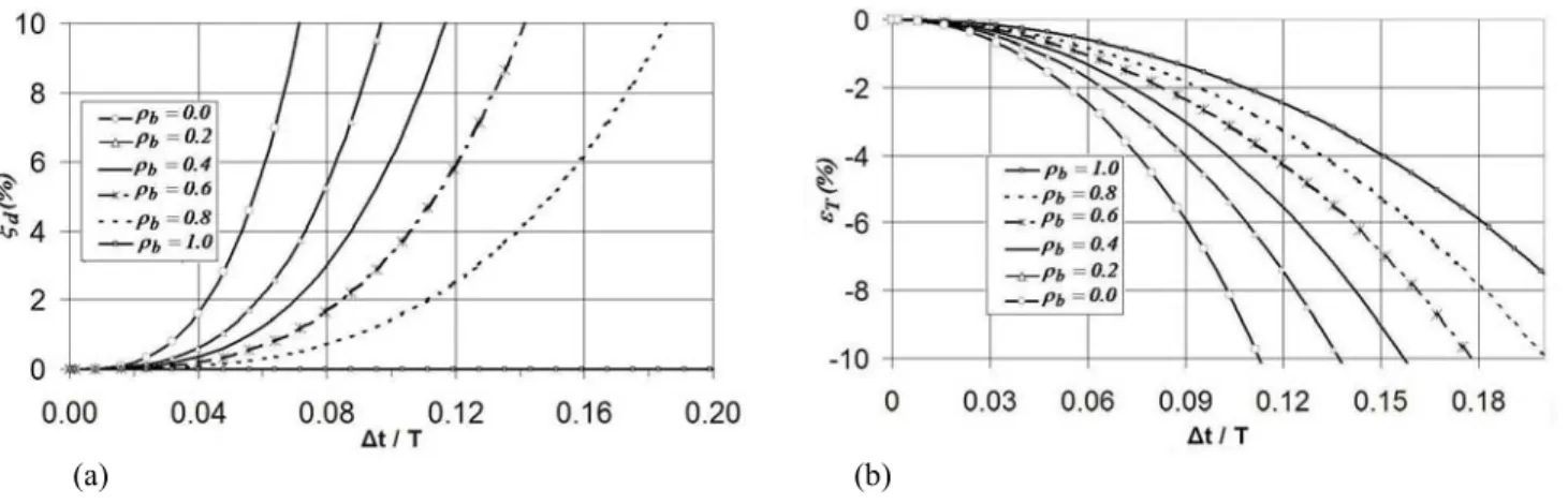
2 1 1 b b = +( −φ)Ω ρ and b ρ φ + = 1 2 . (26) (a) (b)
Figure 1: Numerical characteristics of the TWS scheme. (a) Parameter φ and the bifurcation limit Ωb function of the spectral radius at bifurcation ρb. (b) Evolution of spectral radius ρ in terms of Ω.
The spectral radius at bifurcation ρb has great importance as it is the one user parameter allowing
control of the numerical dissipation, so the characteristic curves are generally given as a function ofρb.
Figure 1b illustrates the variation in spectral radius as a function ofρb. Forρb =0, the high-frequency
response will be nearly annihilated in one step time.
(a) (b)
Figure 2: Errors associated to the TW scheme. (a) Numerical damping ratio. (b) Relative period error.
Because time integration schemes are approximation methods, they introduce errors on the amplitude and on the period of the solution. These errors (11) are reported in Fig. 2.
(
1)
( ); e ( )2 1
eξ = −φ Ω+Ο Ω2 Ω =Ο Ω2 . (27)
The relative period error is shown in the Fig. 2b for different values of ρb, and in function of the
non-dimensional time step ( T
t ∆
). It is interesting to note that for all values of ρb, the relative period error is negative (period shortening). The period shortening increases from a minimum value when
1 =
b
ρ to a maximum value when ρb =0. The TW scheme is second order accurate only if ρb =1, see
Eq. (27).
3.4 Summary of the different schemes
Table 1 summarizes the analysis of the three different time integration schemes (CD, TW and HC). For Ωb =2, TW scheme and HC scheme are spectrally equivalent to the CD method. Moreover, the TW critical time step is globally lower than the HC critical time step, which in turn, is globally lower than the CD critical time step.As a consequence, the TW method is globally the most expensive. The CD method being the reference non dissipative method, the difference between the internal forces of the TW or of the HC and the CD scheme for the free undamped system corresponds to the numerical damping. The TW and the HC schemes are low-pass filters as the relation (27) shows that the higher the frequency, the larger the damping (proportional to the square of the frequency). Another fact is that TW damping depends on the displacements while HC damping depends on the displacement difference. ) x x ( t K F F x t 2 1 K F F n 1 n 2 2 CD int HC int n 2 2 CD int TW int − = − ⎟ ⎠ ⎞ ⎜ ⎝ ⎛ − = − + ω ∆ β ω ∆ φ . (28)
As a consequence, the TW scheme is generally more dissipative than the HC scheme. Table 1:
Comparison between CD, TW and HC schemes Scheme Scheme
order
Control parameter
Period error Critical time step Modified balance equation Bifurcation pulsation CD 2 - shortening max s 2 ω γ no Ωb =2 TW (2 if φ1 =1) ρb(φ) shortening max s 2 φω γ no b = 2 ≤2 φ Ω HC 2 ρb(β,γ,αM ) shortening or elongation max s b ω γ Ω yes Ωb ≤2
5. Numerical examples
The three explicit schemes have been implemented in Metafor, which is an object-oriented finite element code. Interest in numerical dissipation is illustrated by numerical examples. Being a conservative non dissipative scheme, the CD scheme is taken as the reference.
5.1 Taylor impact test
The Taylor impact test consists of the impact of a cylindrical projectile against a rigid wall. Originally, it has been used as a means for determining the dynamical yield strength of metals. Now, it is mostly used as a means for validating plasticity models and time integration schemes. Length and diameter of the projectile are respectively L = 0.0324 m and D = 0.0064 m. The material characteristics of the projectile are: density = 8930 Kg/m³, Young Modulus = 117 GPa, Poisson coefficient = 0.35, yield strength = 0.4 GPa and linear hardening coefficient = 0.1 GPa. Initial velocity of the projectile is
227 m/s. Due to symmetry, only one quarter of the projectile is considered. The projectile is discretized by 48x12 elements. The simulation time is 80 sµ .
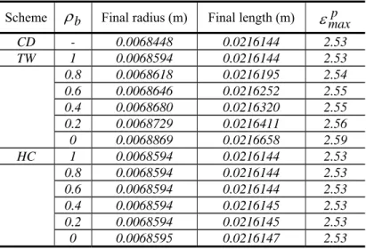
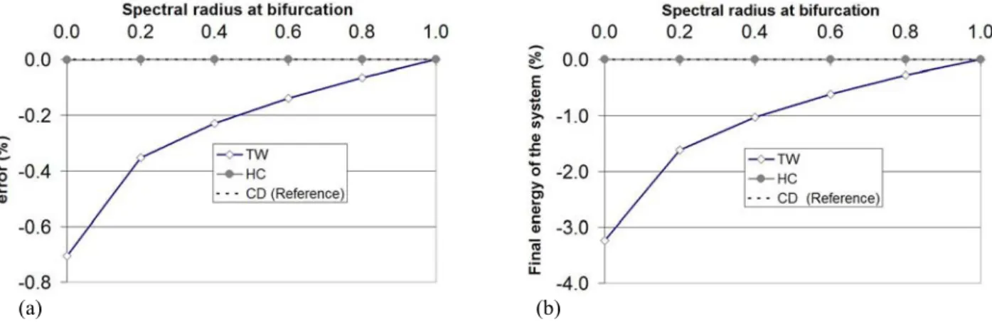
The results (Table 2) show that there is no significant difference in the final radius of the impact side after impact (maximal error=0.6% ), in the final length of the bar (maximum error = 0.2%) as well as in the corresponding final equivalent plastic deformation (maximal error = 2.4%).
The plastically dissipated energy (Fig. 3a) as well as the final elastic energy shows (Fig. 3b) that when the numerical dissipation increases, there is a low decrease in the system energy (plastically and elastic) only for the TW scheme (≤ 1 %) while there is no difference for the HC scheme.
Figure 4 illustrates that, in general, the computational time or the number of time steps increases as the dissipation increases. The CD and the TW schemes for ρb =1 bear the same results either for the number of time steps or the CPU time. In general case, the TW scheme is more expensive than the HC scheme since the bifurcation limit is lower, which induces more time steps.
Table 2:
Final results of the Taylor bar for different schemes and different ρb Scheme ρb Final radius (m) Final length (m) εmaxp
CD - 0.0068448 0.0216144 2.53 TW 1 0.0068594 0.0216144 2.53 0.8 0.0068618 0.0216195 2.54 0.6 0.0068646 0.0216252 2.55 0.4 0.0068680 0.0216320 2.55 0.2 0.0068729 0.0216411 2.56 0 0.0068869 0.0216658 2.59 HC 1 0.0068594 0.0216144 2.53 0.8 0.0068594 0.0216144 2.53 0.6 0.0068594 0.0216144 2.53 0.4 0.0068594 0.0216145 2.53 0.2 0.0068594 0.0216145 2.53 0 0.0068595 0.0216147 2.53
Let us now analyze the pressure histories (Fig. 5a) of the node A which is located at the center of the rear side of the bar and let us see the influence of the numerical dissipation. It appears that the TW scheme smoothes the high frequencies more than the HC scheme. Figure 5b illustrates the pressure history for the TW scheme and a spectral radius at bifurcation equals to 0.8. It appears that to obtain the same degree of high-frequency smoothing with a HC scheme, a lower spectral radius at bifurcation (0.2) has to be used. This demonstrates the high filtering capabilities of the TW scheme with regard to the HC scheme as it was already shown theoretically in section 3.4.
(a) (b)
Figure 3: Analysis of the energy balance for the Taylor’s impact problem (a) Relative error (%) on plastically dissipated energy. (b) Relative error on final reversible energy.
(a) (b)
Figure 4: Computational costs of the schemes for the Taylor’s impact problem (a) Comparison of the number of time steps. (b) Comparison of CPU time (Intel ®, Pentium 4CPU 2.20 GHz, 2.22 GHz, 1 GB of Ram).
(a) (b)
Figure 5: Comparison of high frequencies smoothing capabilities. (a) Smoothing at maximum capability for each scheme. (b) Same degree of smoothing with differentρb.
5.2 Impact of aluminum spherical projectile onto a steel target
Let us consider an aluminum spherical projectile impacting a steel target at a speed of 600 m/s. The projectile diameter is 9 mm. The target diameter and thickness are respectively 60 mm and 1 mm.
The target is made of steel (density = 7870 Kg/m³, Young Modulus = 210 GPa, Poisson coefficient = 0.3, Yield strength = 0.75 GPa, Linear hardening coefficient = 1.15 GPa) and the projectile is made of aluminum (density = 2710 Kg/m³, Young Modulus = 69 GPa, Poisson coefficient = 0.3, Yield strength = 0.29 GPa, Linear hardening coefficient = 0.055 GPa). Frictional contact is treated with a penalty scheme (normal and tangential penalty values are set to 1E+06). Spectral radii used in simulations are respectively 0.0, 0.6 and 1.0. DC is the reference scheme.
The material response at high velocity impact is analyzed for the different schemes. Figure 6 shows the simulation setup and the penetration process at two different times, corresponding to 50 and 100% of the kinetic energy plastically dissipated. The corresponding equivalent plastic strains are illustrated. Deformations are localized at the impact zone and the target underwent a great bulging phenomenon (Fig. 6c). Let us note that no failure model is used, which explain the large plastic strain observed to stop the projectile.
Considering the kinetic energy of the projectile (Fig 7a), except for the HC scheme with spectral radius equal to one, which exhibits a slight energy difference at the end, the energy, function of time is identical for all schemes: the initial kinetic energy is completely dissipated by plastic behavior.
(a) (b) (c)
Figure 6: Penetration mechanism (DC scheme) (a) t =0µs (b) t =6.5µs(50% of the initial kinetic energy dissipated (c) t =48µs(end of penetration mechanism, 100% of the initial kinetic energy dissipated
Let us examine the acceleration at the center of the bullet. For spectral radius equal to one (Fig. 7b), results are the same for the DC and for the TW, but the HC bears oscillations with higher amplitudes and higher frequency than the two other schemes. As dissipation increases, high frequency oscillations are attenuated. The TW presents the highest filtering capabilities (Fig. 7c,d) for the same spectral radius. In particular, it is worth noticing that numerical dissipation constrain the acceleration to negative values, while the DC scheme exhibits oscillations leading to positive values of the acceleration.
Table 3 gives the final displacement of the center node of the sphere in the impact direction and the final equivalent plastic strain. As dissipation increases, the equivalent plastic strain decreases but
there is no difference in the final displacement of the bullet center. Except for HC (ρb =1), the equivalent plastic strains are of the same order. From this observation it can be stated that the numerical oscillations result in an over-estimation of the plastic strains. Numerical dissipation can be used to reduce these oscillations and improve the accuracy of the solutions.
(a) (b)
(c) (d)
Figure 7: Comparison of different schemes - (a) Energy function of time; - Acceleration of the center node of the sphere respectively for (a) ρb =1 , (b) ρb =0.6 and (c) ρb =0.0
Table 3:
Final results for different schemes and different ρb
Scheme ρb
Final displacement of the center of the sphere (mm) p max ε CD - 10.267 4.24 TW 1 10.270 3.85 0.6 10.245 3.58 0.0 10.241 3.26 HC 1 10.284 30.00 0.6 10.260 4.11 0.0 10.260 3.33
6. Conclusions
In this paper, it has been shown that the TW scheme is a more powerful scheme for smoothing high frequencies than the HC scheme. For spectral radius different from one, although the TW is a first-order scheme contrarily to the HC which is a second-order scheme, it gives satisfactory results without losing accuracy. Nevertheless, numerical dissipation is a tool to be used with precaution as it can lead to a loss of accuracy when dissipation increases.
The TW scheme becomes more expensive than the HC scheme when the spectral radius at bifurcation departs from one, but this drawback is balanced by the fact that the same degree of dissipation is reached for a higher spectral radius with the TW scheme.
The TW scheme with spectral radius at bifurcation equal to one is a second order non-dissipative, conservative scheme and is as efficient as the CD scheme.
Numerical schemes have been studied to demonstrate the robustness and accuracy of the HC and TW schemes. For simulations of ballistic impact, numerical dissipation has been used extensively to reduce the oscillations due to finite-element spatial discretizations.
References
[1] Belytschko T. and Hughes T. Computational Methods for Transient Analysis. North Holland; 1983. [2] Hughes T. The Finite Element Method. Prentice Hall; 1987.
[3] Noels L. Contributions to energy-conserving time integration algorithms for non-linear dynamics (in French). PhD Thesis, University of Liège 2004.
[4] Chung J., Lee J.M. A new family of explicit time integration methods for linear and non-linear structural dynamics. Int J Numer Methods Eng 1994; 37:3961-3974.
[5] Hulbert G.M., Chung J. Explicit time integration algorithms for structural dynamics with optimal numerical dissipation. Comput Methods Appl Mech Eng 1996; 137:175-188.
[6] Daniel W.J.T. Explicit/implicit partitioning and a new explicit form of the generalized alpha method. Communication Numer Methods Eng 2003; 19:909–920.
[7] Noels L., Stainier L., Ponthot J.-P. Combined implicit/explicit algorithms for crashworthiness analysis. Int J Impact Eng 2004;30:1161–1177.
[8] Noels L., Stainier L., Ponthot J.-P. Combined implicit/explicit time-integration algorithms for the numerical simulation of sheet metal forming. J Comput and Appl Mathematics 2004; 168: 331-339.
[9] Tchamwa B. Contribution à l’étude des méthodes d’intégration directe explicites en dynamique non-linéaire des structures (in French). PhD Thesis, University of Nantes 1998.
[10] Soive A. Apports à la méthode des éléments finis appliqués aux calculs de structures en dynamique rapide et amortissement numérique (in French). PhD Thesis, University of Bretagne Sud 2003.
[11] Rio G., Soive A., Grolleau, V. Comparative study of numerical explicit time integration algorithms. Adv Eng Software 2005; 36:252 – 265.
[12] Nsiampa N. Comparison of explicit time integration schemes for impact problems (in French). Master Thesis, University of Liège 2006.
[13] Erwin S., de Borst R., Hughes T.J.R. editors. Encyclopedia of computational mechanics, vol. 2: Solids and structures, Wiley; 2004.