Simulation-based inference and nonlinear canonical analysis in financial econometrics

Thèse présentée à la Faculté des études supérieures

en vue de l’obtention du grade de Philosophiae Doctor (Ph.D.)

en sciences économiques

f évrier 2005

Simulation-based Inference and Nonlinear

Canonical Analysis

in

financial Econometrics

par

Pascale Valéry

Département de sciences économiques

Faculté des arts et des sciences

E,

u5’I

o

o

db

de Montréal

Direction des bibliothèques

AVIS

L’auteur a autorisé l’Université de Montréal à reproduire et diffuser, en totalité ou en partie, par quelque moyen que ce soit et sur quelque support que ce soit, et exclusivement à des fins non lucratives d’enseignement et de recherche, des copies de ce mémoire ou de cette thèse.

L’auteur et les coauteurs le cas échéant conservent la propriété du droit d’auteur et des droits moraux qui protègent ce document. Ni la thèse ou le mémoire, ni des extraits substantiels de ce document, ne doivent être imprimés ou autrement reproduits sans l’autorisation de l’auteur.

Afin de se conformer à la Loi canadienne sur la protection des renseignements personnels, quelques formulaires secondaires, coordonnées ou signatures intégrées au texte ont pu être enlevés de ce document. Bien que cela ait pu affecter la pagination, il n’y a aucun contenu manquant. NOTICE

The author of this thesis or dissertation has granted a nonexclusive license allowing Université de Montréal ta reproduce and publish the document, in part or in whole, and in any format, solely for noncommercial educational and research purposes.

The author and co-authors if applicable retain copyright ownership and moral rights in this document. Neither the whole thesis or dissertation, nor substantial extracts from it, may be printed or otherwise reproduced without the author’s permission.

In compliance with the Canadian Privacy Act some supporting forms, contact information or signatures may have been removed from the document. While this may affect the document page count, t does flot represent any Ioss of content from the document

©

Cette thèse intitulée

Simulatïon-based Inference and Nonlinear Canonicat

Analysis in Financial Econometrics

présentée par: Pascale Valéry

a été évaluée par un jury composé des personnes suivantes

Nour Méddahi: _{président-rapporteur}

(Université de Montréal) Jean-Marie Dufour: _{directeur de recherche}

(Université de Montréal) Christian G ouriéroux: _{codirecteur de recherche}

(University of Toronto) Sylvia Gonçalves: _{membre du jury}

(Université de Montréal) Lynda Khalaf: _{examinateur externe}

(Université Lavai) Christian Léger: _{représentant du doyen de la FES}

L’objectif de cette thèse est d’éttidier des techniques d’inférence, classiques et par simulation, en échantillons finis dans le contexte de modèles utilisés en finance.

Dans le premier essai nous introduisons une méthode d’estimation simple, dispo nible en forme fermée, fondée sur la méthode des moments pour une famille générale de modèles de régression à volatilité stochastique, qui rend possible l’implémentation de procédures d’inférence simulées relativement couteuses en calcul. L’estimateur dé veloppé dans cet essai est fondamentalement un estimateur des moments en 2 étapes, qui utilisent les résidus d’une regression préliminaire pour évaluer les conditions de moments de deuxième étape. Sous des conditions de régularité très générales, nous montrons que cet estimateur en 2 étapes est asymptotiquement normalement distribué et en particulier sa matrice de covariance asymptotique ne dépend pas de la distribution de l’estimateur de première étape.

Dans le deuxième essai, nous exploitons la forme fermée de l’estimateur des mo

ments proposé pour implémenter des techniques d’inférence simulée telles que la tech niques des tests de Monte Carlo [cf. Dwass (1957), Barnard (1963), Birnbaurn (1974)]. En particulier, les tests de Monte Carlo maximisés [cf. Dufour(2002)] autorisent des statistiques de tests dont la distribution dépend de paramètres de nuisance. Dans cette procédure, nous définissons une fonction p-value simulée comme fonction des para mètres de nuisance (sous l’hypothèse nulle), et nous montrons que maximiser cette dernière par rapport aux paramètres de nuisance rapporte un test exact, indépendam ment de la taille de l’échantillon et du nombre de réplications utilisées. En particulier, nous implémentons les trois procédures de tests classiques- le test de type Wald, le test

de type score et le test de type LR- ainsi que le test de type c(c) introduit par Neyman (1959). Nous proposons également un test de spécification pour le processus de volati lité qui distingue entre une spécification linéaire de la volatilité contreune spécification alternative à intégration fractionnaire.

Dans le troisième essai, nous estimons le modèle de volatilité stochastique par in férence indirecte [cf Srnith (1993), Gouriéroux, Monfort and Renault (1993)] sous des

n

conditions non regulières. En effet, la condition de rang du jacobien de la fonction de lien asymptotique n’est pas de plein rang en des valeurs isolées du paramètre d’intérêt, condition requise pour que la théorie distributionelle standard dérivée par Gouriéroux, Monfort and Renault (1993) reste valide. En particulier, l’estimateur auxiliaire entrant dans la fonction objectif du critère d’inférence indirecte est fondé sur des conditions de moment qui deviennent nonlinéairement redondantes sous l’hypothèse nulle d’ho moskédasticité du processus de volatilité. La matrice de covariance de l’estimateur auxiliaire ainsi que celle des statistiques de Wald et du score deviennent singulières et non inversibles au sens usuel. Pour remédier à ce problème, nous implémentons des techniques de régularisation dont celle proposée par Ltitkepohl et Burda (1997) qui consiste à prendre un estimateur de rang réduit pour la matrice de covariance de la sta tistique de Wald fondé sur l’inverse généralisée de Moore-Penrose. Les techniques de régularisation proposées permettent aux statistiques de test de rester calculables sous des conditions non régulières. Cependant, la théorie distributionnelle développée par Gouriéroux, Monfort et Renault (1993) n’est plus garantie sous des conditions non ré gulières. Par conséquent, nous combinons des techniques d’inférence par simulation telles que les tests de Monte Carlo maximisés aux statistiques de test modifiées pour rapporter une procédure inférentielle valide en présence d’estimateurs de covariance de rang réduit.

Dans le quatrième essai, nous caractérisons complètement les équations différen tielles stochastiques pour lesquelles les fonctions propres du générateur infinitésimal sont des polynômes dans la variable dépendante. En particulier, des transformations affines du processus d’Omstein-Uhlenbeck, du processus de Cox-Ingersoll-Ross et du processus de Jacobi appartiennent à cette famille d’équations différentielles stochas tiques. De tels processus exhibent une structure très particulière des fonctions de dérive et de volatilité de même qu’une forme particulière des valeurs propres.

Dans le cinquième essai, diverses méthodes d’estimation à partir de données dis crètes sont inspectées pour estimer un processus de Jacobi appartenant à la classe des processus de diffusion dont les fonctions propres sont des polynômes . Les propriétés

distributionnelles de ce processus autant que sa décomposition canonique non linéaire sous-tendent les méthodes d’estimation retenues. Plus précisément, nous proposons une procédure du maximum de vraisemblance approché fondée sur les fonctions propres. Cette méthode de quasi-vraisemblance est alors comparée à la méthode des moments de Kessler et Sorensen (1999). En effet, alors que nous approchons la fonction de tran sition inconnue de données discràtes provenant du processus de Jacobi, ces derniers utilisent la décomposition spectrale pour approcher la fonction score inconnue. Des méthodes d’estimation simulées sont aussi considérées parmi lesquelles la méthode des moments simulés et la méthode d’inférence indirecte. Les propriétés statistiques de ces divers estimateurs sont comparées dans des expériences de Monte Carlo.

Mots clés: volatilité stochastique; volatilité à intégration fractionnaire; méthode des moments; tests exacts; test c(c); inférence indirecte; inverses généralisées; processus dc diffusion; processus de Jacobi; analyse canonique non-linéaire.

$ummary

The objective of this thesis is to study standard and simulation-based inference techniques which are valid in finite samples for models used in finance.

In the first essay, we study a simple moment estimator, available in closed fomi for general regression models with stochastic volatility models This easy-to-use estimator allows for simulation-based inference techniques which can be computationally expen sive. Using residuals from a preliminary regression, the parameters of the stochastic volatility (SV) mode! are then evaluated by a method-of-moment estimator based on three moments (2S-3M) for which a simple closed-form expression can be derived. Under general regularity conditions, we show the two-stage estimator is asymptotically normally distributed. An interesting and potentially useful feature of the asymptotic distribution stems from the fact its covariance matrix does not depend on the distribu tion ofthe conditional mean estimator.

In the second essay, we exploit the closed-form expression of the moment esti mator for the parameters of the SV mode! to implement simulation-based inference techniques sucli as Monte Carlo (MC) tests

_[

see Dwass (1957), Barnard (1963), Bim baum (1974)]. More specifically, maxirnizedMC tests [see Dufour(2002)] allow for test statistics whose distribution may depend on nuisance parameters. In this procedure, we define a simulated p-value function which is not pivotal under the nuli hypothesis and we show that maximizing this p-value w.r.t. nuisance parameters does provide an exact test, irrespective of the sample size and the number of replications used. We imple ment the three standard tests- the Wald-type test, the score-type test and the likelihood ratio-type test- but a!so a c(a)-type test introduced by Neyman (1959). We also pro pose a specification test for the volatility process which discriminates between a Ïinear Gaussian specification for the volatility against afractionaÏÏy integrated Gaussian ai temative.

In the third essay, we estimate the SV model by indirect inference [sec Smith (1993), Gouriéroux, Monfort and Renault (1993), henceforth (GMR)] under nonregu!ar conditions. More specifically, the rank ofthejacobian ofthe asymptotic binding func

tion is flot of fuIl-columri rank at isolated values of the parameter of interest whereas this condition is required for the standard distributional theory dcrived by GMR(1993) to hold. Indeed, the auxiliary estimator which enters the second step objective ente-non in the indirect estimation procedure is based on moment conditions which become nonlinearly redundant under the nuil hypothesis of homoscedasticity of the volatility process. As a result, the covariance matrix become singular and non invertible in the usual sense. Therefore, we propose to regularize the covariance matnix by resorting to a reduced rank matrix estimator based on generalized inverse among which the Moore Penrose inverse proposed by Lutkepohl and Burda (1997). We also propose two slightly different regularization techniques among which one that displays good power proper tics. Furthcr, unlike the nonregularized test statistics, the modifled statistics can aiways be computed under nonregular conditions. However, although the regularization tech niques help in keeping the test statistics computable despite sorne singulanity issues, they do not ensure a 2 distribution for the modified statistics anymore. As a resuit, the distributional resuits developed by GMR (1993) become useless when thejacobian of the asymptotic binding function does not satisfy the required rank condition. One way to overcome this difficulty and stiil provide valid critical points and p-values, is to re sort on mctximized Monte Carlo tests which achieves in controïling for size distortions irrespective of nuisance parameters in the distribution of the test statistic.

In the fourth essay, we characterize the one-dimensional stochastic differential equations, for which the eigcnfunctions of the infinitesimal generator are polynomi als in y. In particular, affine transformations of the Omstein-Uhlenbeck process, the Cox-Ingersoll-Ross process and the Jacobi process belong to this stochastic differen tial equations family. Such processes exhibit specific pattems ofthe drift and volatility functions together with a particular form ofthe eigenvalues.

In the fifth essay, we consider a discretely sampled Jacobi process appropriate to specify the dynamics of a process with range [0,1], such as a discount coefficient, a regime probability, or a state price. The discrete time transition of the Jacobi process does not admit a closed form expression and therefore the exact maximum likelihood

G,

is infeasible. Wc first review a characterization ofthe transition function based on non linear canonical decomposition. They allow for approximations of the log-likelihood function which can be used to define a quasi-maximum likelihood estimator. The finite sample properties of this estimator are compared with the properties of other estima-tors proposed in the literature, such as the Kessier and Sorensen’s estimator which is a method of moments which also exploits the nonlinear canonical decomposition to approximate the unknown score function [sec Kessler and Sorensen (1999)]. It is also compared with generalized method of moments (GMM) estimator, simulated method of moments (SMM) estimator, or indirect inference estimator.

Key words: stochastic volatility; fractionally integrated volatility; moment estima tor; exact tests; c(c)-test; indirect inference; generalized inverses; diffusion processes; Jacobi process; nonlinear canonical analysis.

o

Remerciements

J’ai de nombreuses personnes et institutions à remercier. Tout d’abord mes direc teurs de recherche, Jean-Marie Dufour et Christian Gouriéroux. J’ai eu beaucoup de chance de pouvoir travailler avec des scientifiques et des personnes de cette envergure. Ces années passées sous leur enseignement m’ont apportée un enrichissement incom mensurable.

Je voudrai également remercier un de mes coauteurs, Eric Renault avec qui

j

‘ai eu beaucoup de plaisir à travailler. J’ai apprécié également son humour et sa grande personalité.

Je voudrai également remercier Nour Méddahi pour m’avoir prodiguée des com mentaires scientifiques très pertinents à plusieurs reprises ainsi que pour son soutien moral.

Je voudrai également remercier George Tauchen de m’avoir procurée les données utilisées dans cette étude.

Je voudrai également remercier les différents organismes qui m’ont accordée bourses et financements sans lesquels je n’aurai pu écrire cette thèse: conseil de recherche en sciences humaines du Canada (CRSH), fonds québécois de la recherche sur la na ture et les technologies, centre intemniversitaire de recherche en économie quantitative (CIREQ), le centre interuniversitaire de recherche en analyse des organisations (CI RANO), l’Institut de finance Mathématique de Montréal (1FM2). Je voudrai également remercier HEC-Montréal pour leur support lors de la rédaction finale de cette thèse.

Je voudrai remercier Abdoulaye Diaw pour son aide en informatique. Je voudrai remercier Jean-Pierre Gerbandier pour son soutien moral.

Je voudrai enfin remercier mon conjoint Sylvain Archambault de m’avoir supportée pendant toutes ces années... Je voudrai remercier finalement mes parents et ma soeur Isabelle de m’avoir encouragée tout au long de ce parcours...

Sommaire

Summaty iv

Remerciements viii

List ofDefinitions, Propositions and Theorems xvii

Introduction

1

Simulation-based Inference techniques

5

1. On a simple closed-form estimator for a stochastic volatility mode! 6

1.1. Introduction 7

1.2. Framework 9

1.3. Closed-form method-of-mornents estimator 11

1.4. Asymptotic distribution 14

1.5. Simu’ation study 19

1.6. Application to Standard and Poor’s price index 20

1.7. Conclusion 21

2. Finite and Large Sample Inferencefor a Stochastic Volatillty Mode!2 26

2.1. Introduction 27

‘This paper is co-authored with Jean-Marie Dufour. 2This paper is co-authored with Jean-Marie Dufour.

2.2. framework 31

2.3. Specification test 34

2.4. Tests and confidence sets 35

2.5. Monte Carlo testing 39

2.6. Simulation results 42 2.6.1. Size investigation 44 2.6.2. Power investigation 46 2.7. Empirical application 48 2.7.1. Data 48 2.7.2. Resuits 48 2.8. Concluding remarks 50

3. Monte Carlo Tests and Regularized Indirect Inference for a Stochastic

Volatïlity Model 57

3.1. Introduction 5$

3.2. Estimation by Indirect Inference 61

3.3. Singularity issues: example ofa stochastic volatility mode! 64

3.4. Regularized Inference 67

3.5. Monte Carlo testing 71

3.6. Simulation resuits 73 3.6.1. Size analysis 74 3.6.2. Power analysis 75 3.7. Empirical application 77 3.7.1. Data 77 3.7.2. Results 7$ 3.8. Concluding remarks 79

II.

Nonlinear Canonical Analysis

$4

4. Diffusion Processes with Polynomial Eigenfunctions4 60

4.1. Introduction 61

4.2. Characterization 62

4.3. Proofoftheproperties 65

4.3.1. The pattem ofthe drifi and volatility functions 65

4.3.2. Expression ofthe eigenvalues 66

4.3.3. The constraints on the parameters 67

4.3.4. Stationary distributions 68

4.3.5. Polynomial eigenfunctions 69

5. A quasi-likelihood approach based on eigenfunctions for a Jacobi

process 76

5.1. Introduction 77

5.2. Distributional properties ofthe Jacobi process . . . 80

5.2.1. lime deformation 80

5.2.2. Canonical decomposition 81

5.2.2.1. Spectral decomposition ofthe infinitesimal generator 81

5.2.2.2. The conditional expectation operator 83

5.2.2.3. Moment conditions 83

5.2.3. Marginal and conditional distributions ofthe Jacobi process 86

5.3. Estimation methods 86

5.3.1. (Approximate) Quasi-maximum likelihood 87

5.3.2. Method of moments 88

5.3.2.1. Selection ofthe moments 88

5.3.2.2. Identification issue $9

5.3.2.3. An exact indirect estirnator 90

5.3.2.4. Generalized-method-of-moments estimator . . . 90

5.3.2.5. Estirnating equations based on eigenfunctions . . 91

4This paper is co-atithored with Christian Gouriéroux and Eric Renault. 5This paper is co-authored with Christian Gouriéroux.

5.3.3. Simulated methods 95 5.3.3.1. The simulated method of moments 95 5.3.3.2. The indirect inference method 96

5.4. Simulation ofthe Jacobi process 97

5.4.1. A truncated Euler scheme 97

5.4.2. Simulation scheme based on time deformation 98

5.4.3. Simulated series 99

5.5. Comparison ofthe estirnators 102

5.5.1. The estimation methods 102

5.5.2. Marginal properties ofthe estimated coefficients 104 5.5.3. Joint distributional properties ofthe estimators ofband c . 111

5.6. Concluding remarks 113

Conclusions générales

14$

PartI 6

1.1 BIAS 23

1.2 VARIANCE 24

1.3 RIVISE 25

2.1 Size ofasymptotic and Monte Carlo tests, specification test 51

2.2 Size ofasymptotic and Monte Carlo tests,H0 a = O 51

2.3 Size ofasymptotic and Monte Carlo tests, H0 a = 0, r O . . . 51

2.4 Size ofasymptotic and Monte Carlo tests, H0 a O, r, = O . . . 52

2.5 Power ofasymptotic and Monte Carlo tests, specification test 52

2.6 Simulated critical values, under H0 : ci O 52

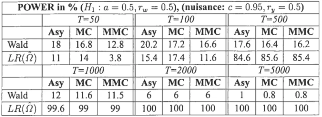
2.7 Power of size-corrected asymptotic and Monte Carlo tests 53 2.8 Power of asymptotic and Monte Carlo tests, fI1 ci = 0.5, ri,, = 0.5,

setl 53

2.9 Power of asymptotic and Monte Carlo tests, H1 ci = 0.5, r 0.5,

setll 54 2.10 Empirical application 54 2.11 Confidence sets 54 3.1 Size 81 3.2 Power 82 3.3 Empirical application $3 Part II 60 xlii

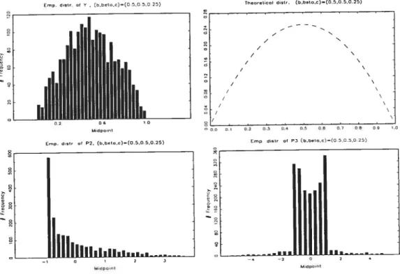
5.1 Summary statistics for y and beta distr 101

5.2 Summary statistics for P1,P2,P3 101

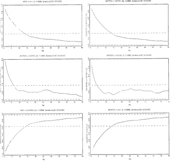
5.3 Sample and theoretical correlations for P1,P2,P3 102

5.4 Standardized variance 114

5.5 Non standardized skewness and kurtosis 115

PartI 6 2.1 Asymptotic and Monte Carlo Power functions, Wald and LR tests . . 55

2.2 Asymptotic and Monte Carlo Power functions, score and C(c) tests . 56

Part 11 60

5.1 Simulated paths, set I 117

5.2 Simulated paths, set II 118

5.3 Empirical marginal distributions, set I 119

5.4 Empirical marginal distributions, set II 120

5.5 Empirical correlations, set I 121

5.6 Cross autocorrelograms, set II 122

5.7 Cross autocorrelograms, set (0.1,0.5,0.03) 123

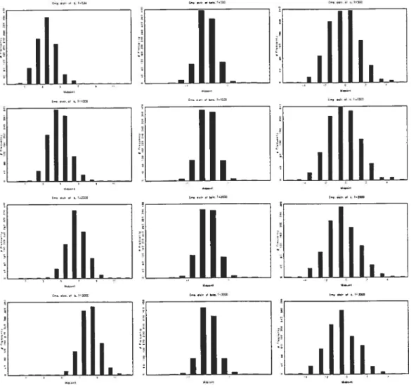
5.8 Standardized marginal sample distribution of ET, set I 124 5.9 Standardized marginal sample distribution of ET, set II 125 5.10 Standardized marginal sample distribution ofQML, set I 126 5.11 Standardized marginal sample distribution ofQML, set II 127 5.12 Standardized marginal sample distribution ofEIG, set I 128 5.13 Standardized marginal sample distribution ofEIG, set II 129 5.14 Standardized marginal sample distribution ofGMM, set I 130 5.15 Standardized marginal sample distribution ofGMM, set II 131 5.16 Standardized marginal sample distribution ofSMM, set I 132 5.17 Standardized marginal sample distribution ofSMM, set II 133

5.18 Standardized marginal sample distribution of II, set I 134 5.19 Standardized marginal sample distribution of II, set II 135 5.20 Standardized joint sample distribution of b and c, ET, set I 136 5.21 Standardized joint sample distribution of b and c, ET, set II 137 5.22 Standardized joint sample distribution of b and c, QML, set I 138 5.23 Standardized joint sample distribution of b and c, QML, set II . . 139

5.24 Standardized joint sample distribution of b and c, EIG, set I 140 5.25 Standardized joint sample distribution of b and c, EIG, set II 141 5.26 Standardized joint sample distribution of b and c, GMM, set I . . 142 5.27 Standardized joint sample distribution of b and c, GMM, set II . . 143

5.28 Standardized joint sample distribution of b and c, SMM, set T 144 5.29 Standardized joint sampÏe distribution of b and c, SMM, set II . . 145

5.30 Standardized joint sample distribution of b and c, II, set I 146 5.31 Standardized joint sample distribution of b and c, II, set II 147

List of Definitions, Propositions and Theorems

1.2.1 Assumption Linear regression with stocliastic volatility 9 1.2.2 Assumption Autoregressive model with stochastic volatility 10

1.2.3 Assumption Gaussian noise 11

1.2.4 Assumption 2 Stationarity 11

1.3.1 Lemma : Moments and cross-moments ofthe volatility process 12

1.3.2 Lemma: Moment equations solution 12

1.3.3 Lemma 2 Higber-order autocovariance functions 13 1.4.1 Assumption : Asymptotic nomality of empirical moments 15 1.4.2 Assumption : Asymptotic equivalence for empirical moments 15 1.4.3 Assumption: Asymptotic nonsingularity of weight matrix 15 1.4.4 Assumption : Asymptotic nonsingularity of weight matrix 15 1.4.5 Proposition : Asymptotic distribution ofmethod-of-moments estimator 16

1.4.7 Proposition : Asymptotic distribution for empirical moments 18

1.4.8 Proposition : Asymptotic equivalence for empiricaÏmoments 18

2.2.4 Proposition : Moments ofthe volatility process 32

2.2.5 Proposition: Estimating equations 33

4.2.1 Assumption : Compactness ofthe infinitesimal operator 62

4.2.2 Proposition : CharacterizationProperty 62

4.2.3 CoroI1ar 64 ProofofLemma 1.3.1 . . . 165 ProofofLemma 1.3.2 . . . 165 ProofofLemma 1.3.3 . . . 166 ProofofProposition 1.4.5 167 ProofofProposition 1.4.7 168 ProofofProposition 1.4.8 172

La thèse traite de divers sujets d’économétrie financière. Elle est divisée en deux parties. La première partie propose des tests simulés en échantillons finis dans le contexte de modèles utilisés en finance (3 essais) tandis que la seconde partie développe des nié thodes d’analyse canonique non linéaire pour des processus de diffusion (2 essais).

Dans la première partie de la thèse nous nous intéressons aux propriétés asympto tiques et en échantillons finis de diverses statistiques de tests dans le cadre du modèle de volatilité stochastique lognormal introduit par Taylor (1986). Depuis, ce modèle a été largement utilisé en finance et plus particulièrement en économétrie de la finance - car

il est directement relié aux processus de diffusion très populaires en finance théorique [cf. Wiggins (1987), Melino and Tumbull (1990), Chernov, Gallant, Ghysels and Tau

chen (2004)]. Cependant, il reste difficile à estimer en particulier quand il est comparé aux modèles de type GARCH [cf. Engle (1982), Boflerslev (1986)] en raison de l’in troduction d’un bruit inobservable dans le processus de volatilité rendant les méthodes d’estimation usuelles -telles le maximum de vraisemblance infaisable. De nombreuses

techniques d’estimation alternatives, quasi-exactes [cf. Nelson (1988), Harvey, Ruiz, and Shephard (1994), Ruiz (1994)], GMM [Melino and Turnbull (1990), Andersen and Sørensen (1996)], ou des techniques d’échantillonage fondées sur la simulation telles que le maximum de vraisemblance simulé [Danielsson and Richard (1993), Daniels son (1994)], ou encore l’inférence indirecte [cf. Gouriéroux-Monfort-Renault(1993)] ou encore la méthode efficace des moments de Gallant et Tauchen (1996), [cf. Gallant, Hsieh, and Tauchen (1997), Andersen, Chung, and Sorensen (1999)] —ou encore des

méthodes bayesiennes [Jacquier, Polson, and Rossi (1994), Kim, Shephard, and Club (1998)] ont alors été proposées dans la litérature afin de contourner cette difficulté mais souvent au prix de complication s computati onelles importantes.

C’est la raison pour laquelle, dans le premier essai nous introduisons une méthode d’estimation simple, disponible en fomie fermée, fondée sur la méthode des moments pour une famille générale de modèles de régression à volatilité stochastique, qui rend possible l’implémentation de procédures d’inférence simulées relativement couteuses

en calcul. L’estimateur développé dans cet essai est fondamentalement un estimateur des moments en 2 étapes, qui utilisent les résidus d’une regression préliminaire pour évaluer les conditions de moments de deuxième étape. Sous des conditions de régularité très générales, nous montrons que cet estimateur en 2 étapes est asymptotiquement nor malement distribué et en particulier sa matrice de covariance asymptotique ne dépend pas de la distribution de l’estimateur de première étape. Suivant des résultats récents sur l’estimation de modèles autorégressifs à volatilité stochastique [cf. Goncalves-Kilian (2004)], les résultats distributionels développés dans cet essai, restent valides en parti culier pour de tels modèles.

Dans le second essai, nous exploitons la forme fermée de l’estimateur des moments proposé pour implémenter des techniques d’inférence simulée telles que la techniques des tests de Monte Carlo [cf. Dwass (1957), Bamard (1963), Bimbaum (1974)]. En particulier, les tests de Monte Carlo maximisés [cf. Dufour (2002)] autorisent des sta tistiques de tests dont la distribution dépend de paramètres de nuisance. Dans cette procédure, nous définissons une fonction p-value simulée comme fonction des para mètres de nuisance (sous l’hypothèse nulle), et nous montrons que maximiser cette dernière par rapport aux paramètres de nuisance rapporte un test exact, indépendam ment de la taille de l’échantillon et du nombre de réplications utilisées. En particulier, nous implémentons les trois procédures de tests classiques -le test de type Wald, le test

de type score et le test de type LR- ainsi que le test de type c(û) introduit par Neyman (1959).Nous procédons alors à des comparaisons entre les techniques asymptotiques et les procédures d’inférence simulées. Les résultats exhibent une meilleure performance du test de type c(). Nous proposons également un test de spécification pour le pro cessus de volatilité qui distingue entre une spécification linéaire de la volatilité contre une spécification alternative à intégration fractionnaire qui présente un intérêt crucial en terme de mémoire longue pour la valorisation d’options [cf. Comte and Renault (1998), Comte, Coutin and Renault (2003), Ohanissian, Russel and Tsay (2003)]. Des expériences de Monte Carlo sont réalisées et suivies par une application empirique sur données journalières pour l’indice de prix composite du Standard and Poor(1928-87).

Dans le troisième essai, nous estimons le modèle de volatilité stochastique par in férence indirecte [cf Smith (1993), Gouriéroux, Monfort and Renault (1993)] sous des conditions non regulières. En effet, la condition de rang du jacobien de la fonction de lien asymptotique n’est pas de plein rang en des valeurs isolées du paramètre d’intérêt, condition requise pour que la théorie distributionelle standard dérivée par Gouriéroux, Monfort and Renault (1993) reste valide. En particulier, l’estimateur auxiliaire entrant dans la fonction objectif du critère d’inférence indirecte est fondé sur des conditions de moment qui deviennent nonlinéairement redondantes sous l’hypothèse nulle d’ho moskédasticité du processus de volatilité. La matrice de covariance de l’estimateur auxiliaire ainsi que celle des statistiques de Wald et du score deviennent singulières et non inversibles au sens usuel. Pour remédier à ce problème, nous implémentons des techniques de régularisation dont celle proposée par Ltftkepohl et Burda (1997) qui consiste à prendre un estimateur de rang réduit pour la matrice de covariance de la sta tistique de Wald fondé sur l’inverse généralisée de Moore-Penrose. Les techniques de régularisation proposées permettent aux statistiques de test de rester calculables sous des conditions non régulières. Cependant, la théorie distributioimelle développée par Gouriéroux, Monfort et Renault (1993) n’est plus garantie sous des conditions non ré gulières. Par conséquent, nous combinons des techniques d’inférence par simulation telles que les tests de Monte Carlo maximisés aux statistiques de test modifiées pour rapporter une procédure inférentielle valide en présence d’estimateurs de covariance de rang réduit. Des résultats de simulation sur la performance des test modifiés sont pré sentés suivies d’une illustration financière pour l’indice de prix composite du Standard and Poor (1928-87).

La seconde partie de la thèse est consacrée à l’analyse canonique non linéaire de processus de diffusion dont le but est d’étudier la dépendance temporelle des proces sus d’une façon moins traditionnelle. Ainsi la décomposition canonique de la distri bution conditionnelle permet d’identifier les directions de corrélation maximale entre les variables canoniques ce qui présente un intérêt statégique en finance empirique en particulier en terme de couverture des risques.

Dans le quatrième essai, nous caractérisons complètement les équations différen tielles stochastiques pour lesquelles les fonctions propres du générateur infinitésimal sont des polynômes dans la variable dépendante. En particulier, des transformations affines du processus d’Omstein-Uhlenbeck, du processus de Cox-Ingersoll-Ross et du processus de Jacobi appartiennent à cette famille d’équations différentielles stochas tiques. De tels processus exhibent une structure très particulière des fonctions de dérive et de volatilité de même qu’une forme particulière des valeurs propres. En outre, des contraintes de stabilité sont imposées sur les paramètres des processus.

Dans le dernier essai, diverses méthodes d’estimation à partir de données discrètes sont inspectées pour estimer un processus de Jacobi appartenant à la classe des proces sus de diffusion dont les fonctions propres sont des polynômes . Ce processus prend des valeurs entre O et I, et semble donc adapté pour modéliser des variables dynamiques bornées telle qu’une probabilité de changement de régime, ou capturer l’évolution d’un prix d’état. Les propriétés distributionnelles de ce processus autant que sa décompo sition canonique non linéaire sous-tendent les méthodes d’estimation retenues. Plus précisément, nous proposons une procédure du maximum de vraisemblance approché fondée sur les fonctions propres. Cette méthode de quasi-vraisemblance est alors com parée à la méthode des moments de Kessler et Sorensen (1999). En effet, alors que nous approchons la fonction de transition inconnue de données discrètes provenant du processus de Jacobi, ces derniers utilisent la décomposition spectrale pour approcher la fonction score inconnue. L’estimateur de quasi-vraisemblance est aussi comparé à la méthode des moments généralisés de Hansen (1982) puisque la décomposition spec trale de l’opérateur d’espérance conditionelle [cf. Hansen and Sheinckman (1995)] et la forme polynomiale des fonctions propres associées fournissent tous les moments conditionels du processus en terme des moments marginaux. Des méthodes d’estima tion simulées sont aussi considérées parmi lesquelles la méthode des moments simulés et la méthode d’inférence indirecte. Les propriétés statistiques de ces divers estimateurs sont comparées dans des expériences de Monte Carlo.

$imulation-based Inference techniques

On a simple closed-form estimator for

a stochastic volatility mode!

1.1.

Introduction

Modelling conditional heteroskedasticity is OIIC of the central problems of financial econometrics. The two main families of models for that purpose consist of GARCH type processes, originally introduced by Engle (1982), and stochastic volatility (SV) models proposed by Taylor (1986). Although the latter may be more attractive— be

cause they are directly connectcd to diffusion processes used in theoretical finance —

GARCH models are mucli more popular because they are relatively easy to estimate; for reviews, see Gouriéroux (1997) and Palm (1996). In particular, evaluating the like lihood function of GARCH models is simple compared to stochastic volatility models for which it is very difficult to get a iikelihood in closed form; sec Shephard (1996), Mahieu and Schotman (1998) and the review ofGhysels, Harvey, and Renault (1996). This is a generai feature of almost ail nonlinear latent variable models, due to the high dimensionahty of the integral defining the hkelihood function. As a resuit, maximum likelihood methods are prohibitively expensive from a computational viewpoint, and alternative methods appear to be required for applying such models.

Since the first discrete-time stochastic volatility models was proposed by Taylor (1986) as an alternative to ARCH models, much progress has been made regarding the estimation of nonlinear latent variable modeÏs in general and stochastic volatil ity moUds in particular. The methods suggested include quasi maximum likelihood estimation [sec Nelson (1988), Harvey, Ruiz, and Shephard (1994), Ruiz (1994)], gen eralized method-of-moments (GMM) procedures [Melino and Tumbuil (1990), Ander sen and Sorensen (1996)], sampling simulation-based techniques — such as simulated

maximum likelihood [Danielsson and Richard (1993), Danielsson (1994)], indirect in ference and the efficient method of moments [Gallant, Hsieh, and Tauchen (1997), An dersen, Chung, and Sørensen (1999)] — and Bayesian methods [Jacquier, Poison, and

Rossi (1994), Kim, Shephard, and Chib (1998),Wong (2002a), Wong (2002b)]. Note also that the rnost widely studied specification in this literature consists ofa stochastic volatility model oforder one with Gaussian log-volatility and zero (or constant) condi tional mean. The most notable exception can be found in Gallant, Hsieh, and Tauchen

(1997) who ailowed for an autoregressive conditional mean and considered a general autoregressive process on the iog-voiatiiity. It is remarkable that ail these methods are highiy noniinear and computer intensive. Impiementing them can be quite complicated and get more so as the number of parameters increases (e.g., with the orders of the autoregressive conditional mean and iog-voiatility).

In this paper, we consider the estimation of stochastic volatility parameters in the context ofa iinear regression where the disturbances follow a stochastic voiatility model of order one with Gaussian iog-voiatiiity. The iinear regression represents the condi tionai mean of the process and may have a fairly general form, which includes for exampie finite-order autoregressions. Our objective is to deveiop a computationaiiy inexpensive estimator that can be easily expioited within a simuiation-based inference procedures, such as Monte Carlo and bootstrap tests.2 So we study here a simple two step estimation procedure which can be described as foilows: (1) the conditional mean model is first estimated by a simple consistent procedure that does take into account the stochastic volatiiity structure; for example, the parameters of the conditionai mean can be estimated by ordinary ieast squares (aithougli other estimation procedures can be used); (2) using residuais from this preliminaiy regression, the parameters of the stochastic model are then evaluated by a method-of-moment estimator based on three moments (2S-3M) for which a simple closed-form expression can be derived. Under generai regularity conditions, we show the two-stage estimator is asymptoticaiiy nor maiiy distributed. Foilowing recent resuits on the estimation of autoregressive modeis with stochastic voiatility [sec, for exampie, sec Theorem 3.1, Gonçalves and Kiiian (2004)], this then entails that the resuit hoids for such models. An interesting and po tentiaily useftil feature ofthe asymptotic distribution stems from the fact its covariance matrix does not depend on the distribution ofthe conditional mean estimator, Le., the estimation uncertainty on the parameters of the conditional mean does not affect the distribution of the voiatility parameter estirnates (asymptotically). The properties of the 2S-3M estimator are aiso studied in a small Monte Cario experiment and compared 2TIis feature is exploited in a companion paper tDufour and Valéry (2004)] where various simulation

with GMM estimators proposed in this context. We find that the 25-3M estimator has quite reasonable accuracy with respect to the GMM estimators: indeed, in several cases, the 2S-3M estimator lias the lowest root mean square error. With respect to computa tional efficiency, the 2S-3M estimator aiways requires less than a second whule GMM estimators may need several hours before convergence obtains (if it does). Finally, the proposed estimator is illustrated by applying it to the estimation of Standard and Poor’s Composite Price Index (1928-87).

The paper is organized as follows. Section 1.3 sets the framework and the main assumptions made. The closed-form estimator studied is described in section 1.3. The asymptotic distribution of the estimator is established in section 1.4. In section 1 .5, we report the results of a small simulation study on the performance of the estimator. Section 1.6 gives an application to the Standard and Poor’s Composite Price Index retum series in Section 5. We conclude in section 1.7. AIl proofs are gathered in the Appendix.

1.2.

Framework

We consider here a regression model for a variable y, with disturbances that follow a stochastic volatility process, which is described below following a notation similar to the one used by Gaflant, Hsieh, and Tauchen (1997).

Assumption 1.2.1 LINEAR REGRE$SION WITH STOCHASTIC VOLATILITY. The process {yt : t

e

N03}follows a stochastic voÏatiÏity modeÏ ofthe type:

YtX+flt, (1.2.1)

= exp(w/2)rzt, _Wt = aw_ + TVt , (1.2.2)

where xj isa k x 1 randomvector independent ofthe variables {r7-_1, z, u-,-, w-,- : T <

t}, and[3, r, {a}1, r are fixed parameters. 3N0refers to the nonnegative integers.

TypicallyYt denotes the first difference over a short time interval, a day for instance, ofthe log-price ofa financial asset traded on securities markets. The regression function x/3 represents the conditional mean oflit (given the past) while the stochastic volatil ity process dctermines a varying conditional variance. A common specification here consists in assuming that x8 lias an autoregressive form as in tlie following restricted version ofthe mode! described by Assumption 1.2.1.

Assumptïon 1.2.2 AUTOREGRESSIVE MODEL WITH STOCHASTIC VOLATILITY. Theprocess {y : L e No}folÏows a stochastic volatiÏity model ofthe type.

L lit — c(yt_ —

)

+u, (1.2.3) j=1 Ut = exp(w/2)Tz, aw_ +TVt , (1.2.4) i=1

where, {c}1, r, {a}1 andT are fixedparameters.

We shah refer to the latter model as an AR-SV(L, L) model. The !ag !engtlis of the autoregressive specifications used in the literature are typically short, e.g.: O and L = 1 [Andersen and Sorensen (1996), Jacquier, Poison, and Rossi (1994),

Andersen, Chung, and Sørensen (1999)], 0 < < 2 and O < L < 2 [Gai!ant, Hsieli, and Tauclien (1997)]. In particuhar, we will devote special attention to the AR-SV(1, 1) mode!: Yt — = C(yti — t) _{+ exp(wt/2)rzt, c} < 1 (1.2.5) = O]t—i +TU a < 1 . (1.2.6) so that Cov(wt,wt+T) = aTy (1.2.7)

where = r/(1 — a2). The basic assumptions described above wi!i lie completed by

j

Assumption 1.2.3 GAUSSIAN NOISE. The vectors (Zj, Ut)’, t N0 ai-e i.i.d. accord

ing toa N[O, 12] distribution.

Assumption 1.2.4 STATIONARITY. Theprocess St = (yt, Wt)’ is srrictÏy stationarv.

The process defined above is Markovian oforder L3 = max(L0, L). Under these

assumptions, the AR-SV(L0, L) is a parametric model with pararneter vector

p =

(,

C1, . . .

,

C, T0, a1, . . .

,

aLt,, ‘r,)’. (1.2.8)

Due to the fact that the model involves a latent variable (Wt), the joint density of the

vector of observations = (iii, •..

,

l/T) is flot available in closed-form because the latter would involve evaluating an integral with dimension equal to the whole path of the latent volatilities.

1.3.

Closed-form method-of-moments estimator

In order to estimate the parameters of the volatility model described in the previous section, we shall consider the moments of the residual process in (1 .2.1), which can 5e estimated relatively easily from regression residuals. Specifically, we wi]1 focus on stochastic volatility model oforder one (L = 1). Set

O = (a, T0, T)’, (1.3.1)

awt_i + TUt

Ut(O) exp(

2 )T0Zt, Vt. (1.3.2)

Model (1.2.1) - (1.2.2) may then be conveniently rewritten as the following identity:

The estimator we will study is based the moments of the process Ut E _Vt(O). The required moments are given in the following lemma.

Lemma 1.3.1 MOMENTS AND CROSS-MOMENTS 0f THE VOLATILITY PROCESS. Under the assumptions 1.2.1, 1.2.3 and 1.2.4 with L = 1, the moments and

cross-moments ofUt = exp(wt/2)T0zt aregiven by thefollowingform;tlas: for k, t and ra

nonnegative integers,

E E(u) _{= T2(k/2/2)!} exp [T/(1 — a2)], k is even,

= O, ïfkisodd, (1.3.4)

k1(mI) E _E(UU+m)

= T0

2(k/2)(k/2)! 2(t/2)(t/2)! exp a2)(k2 + t2 +

2ktaT.3.5)

if k and t are even, and ,k,t(mI&) = O

f

k or t is odd.

Ontakingk=2,k=4,k=rt=r2andrn=1,weget:

t2() = E(u)=Texp[r/2(1—a2)], (1.3.6)

E(u) = 3rexp{2r/(1 — a2)] (1.3.7)

2,2(10) = E[uu1] = rexp[T/(1 - a)]. (1.3.8)

An important observation here cornes from the fact the above equations can be explic itly solved for a, rand r. The solution is given in the following lemma.

Lemma 1.3.2 MOMENT EQUATIONS SOLUTION. Under the assumptions offropo 4Expressions for the autocorrelations and autocovariancesofuwere derived by Taylor(1986,Sec

tion 3.5) and Jacquier, Poison, and Rossi (1994). The latter authors aiso provide the higher-order mo ments _E[In], whiie generai formulas for the higher-order cross-moments of a stochastic voiatihty process are reported (without proof) by Ghyseis, Harvey, and Renault (1996). For compieteness, we give a relatively simple proof in the Appendix.

sition 1.3.1, we have:

— 1og[i22(1I)] + log [4(&)/(3I2())]

1 1 3 9 a log [4(9)/(32()2)] 31/4 _KO” = _[L4(/4 (1.3.10) j 1/2

=

[ti

— a2)log [4(9)/(32(o)2)]] . (1.3.11)

From lemmas 1.3.1 and 1.3.3, it is easy to derive higher-order autocovariance func tions. In particular, for later reference, we will find useful to speil out the second and fourth-order autocovariance functions.

Lemma 1.3.3 HIGHER-ORDER AUTOCOVARIANCE FUNCTIONS. Under theassztrnp

tions ofProposition 1.3.1, let X, = (Xii, X2,, X3)’ where

—

(&),

X2 = — bt4(9), X3t ₌

— 22(1). (1.3.12)

Then the covariances (r) Cov(X,, Xj,t+T), i = 1, 2, 3, are given by:

7y(T) t1(9)[exp(yaT) — 1] (1.3.13) 72(T) = tJ)[exp(47ciT) — 1] Vr 1, (1.3.14) = 2,2(10)[exp(7(1 + a)2aT_l) — 1], Vr 2, (1.3.15) where y = r/(1 — a2).

Suppose now we have a preliminary estimator of /3. For example, for the au toregressive model (1.2.3)- (1.2.4), estimation ofthe equation (1.2.3) yields consistent

asymptotically normal estimators of [3; sec Theorem 3.1, Gonçalves and Kilian (2004) and Kuersteiner (2001). 0f course, other estimators ofthe regression coefficients may be considered. Given the residuals

it is then natural to estimate_{2(), ji.(&) and i22(lIO) by the corresponding empirical} moments:

[L2Z,

This yields the following estimators ofthe stochastic volatility coefficients:

= log[2(1)] + log [4/(3)] - 1 (1 3 17) 10g [4/(3)] 1/4 / 1/4 _3_2_(32 14 _\/L4J 1/2

[t’

- à2)log [4/(3)]] . (1.3.19)

Clearly the latter estimates can 5e quite easy to compute as soon as the estimator used to compute the residuals = — x is also easy to obtain (e.g., it is a Ieast squares

estimator).

1.4.

Asymptotic distribution

We will 110W study the asymptotic distribution of the moment estimator defined in

(1.3.17) - (1.3.19). For that purpose, it will be convenient to view the latter as a special

case of the general class of estimators obtained by minimizing a quadratic form of the type:

Mr(9) = [TtÛT) - (0)j’T[TtÛT)

- (6)] (1.4.1)

where

₍₎

is a vector of moments, YT(UT) is the corresponding vector of empirical moments based on the residual vector ÛT =

(,

•..

,

u)’, and 2T is a positive

definite (possibly random) matrix. 0f course, this estimator belongs to the general family of moment estimators, for which a number ofgeneral asymptotic general resuits do exist; see Volume 1, Chapter 9, Gouriéroux and Monfort (1995b) and Newey and McFadden (1994). However, we need to account here fortwo specific features, namely:

(1) the disturbances in (1.2.1) follow a stochastic volatility model, and the satisfaction of the relevant regularity conditions must be checked; (2) the two-stage nature of the procedure where the estimator of the parameter of the conditional mean equation is obtained separately and may not be based on the same objective function as the one used to estimate 0. In particular, it is important to known whether the the estimator of conditional mean parameter lias an effect on the asymptotic distribution of the estimator of 0.

To speli out the properties ofthe estimatorT(f2T) obtained by minimizingMT(O), we will consider first the following generic assumptions, where 0 denotes the “truc” value ofthe parameter vector 0.

Assumption 1.4.1 ASYMPTOTIC NORMALITY 0F EMPIRICAL MOMENTS.

[TtUT) - (0o)] N[O,

]

(1.4.2)

where UT (ni, ... _, n)’ and

= 11m _E{T[T(UT) - (0)] [T(UT) - (0)]’}. (1.4.3)

Assumption 1.4.2 ASYMPTOTIC EQUIVALENCE FOR EMPIRICAL MOMENTS. The randoin vector V’[.T(ÛT) —

,u(00)]

is asyrnptoticaÏly eqitivalent 10 v”[T(UT)

—

t(0o)] ,

i.e.

p1im{[T(ÛT)

- (0)]

- [r(UT) - (0)]

}

=0. (1.4.4)

T—oo

Assumption 1.4.3 ASYMPTOTIC NONSINGULARITY 0F WEIGHT MATRIX. plim(.QT)= !2wheredet(f2)O.

Assumption 1.4.4 ASYMPTOTIC NONSINGULARITY 0F WEIGHT MATRIX. i(0o) is Iwice continuously diffèrentiabÏe in an open neighborhood oJ’00 andthe Jacobian matrix P(00) hasfïtlÏ rank, where P(0) --.

Given these assumptions, the asymptotic distributionof?T(f2T) is determined by a standard argument on method-of-moments estimation.

Proposition 1.4.5 ASYMPTOTIC DISTRIBUTION 0F METHOD-0F-MOMENTS ESTI MATOR. Under the assumptions 1.4.1 to 1.4.4,

v[T(f2) -

o]

N[O,

V(OoIf2)]

(1.4.5)

where

V(91f2)

= [P(O)f2P(&)’j’ P(O)f2f2!2P(8)’ [P()f2P(O)’]’ (1.4.6)

P(8) = . If furthermore, (z) P(9) is a square mati-ix or (ii,.) f2 is nonsinguÏar and f2 = f2:’, then

= V(O). (1.4.7)

As usual, V,. (On) is the smallest possible asymptotic covariance matrix for a method of-moments estimator based on IVfT_(e). The latter, in particular, is reached when the dimensions ofj and O are the same, in which case the estimator is obtained by solving the equation

gT(UT)

Consistent estimators V(001S2) and V0(00) can be obtained on replacing 0c and 12, by consistent estimators.

A consistent estimator ofS7 can easily be obtained [see Newey and West (1987b)] by a Bartlett kemel estirnator, i.e.:

K(T) *=Fo+Z(1_K()+l)(Pk+Pk) (1.4.8) where = _{9tk(Û) - (O)][g(û) -t=k+1

with O replaced by a consistent estimator 0T of O. The truncation parameter K(T) =

6T’3 is allowed to grow with the sample size such that:

K(T) 11m , =0, T—œ T’i2

[sec White and Domowitz (1984)]. A consistent estimator 0fV (Os) is then given by:

= [P(T)&’P(T)’]’. (1.4.9)

The main problem here consists in showing that the relevant regularity condi tions are satisfied for the estimator O = (â, iJ, i)’ given by (1.2.5)-(1.2.6) for the parameters of a stochastic volatility moUd of order one. In this case, we have (O) = [/12(0), /14(6), /12,2(110)], i —T 2 T Lt=it gTWT)=gt(UT)= 1T22 (1.4.10)

Z=1

LUt1 1 çT 2 T T Zt=i t T(UT) = = (1.4.11) i T 22 zt=1

where

g(ÛT)

= [û, û, ûû_1], and _{gt(UT) =} [ri,

r4, rLu_1]’.

Since the number of moments used is equal to the number of parameters (three), the moment estimator can be obtained by taking 2T equal to an identity matrix so that Assumption 1.4.3 automatically holds. So the main problem consists in showing that the assumptions 1.4.1 and 1.4.2 are satisfied. for that, it wiIl useful to show the following lemma.

O

Assumption 1.4.6 EXISTENCE 0F MOMENTS. Let: p1im Xt = u2,(O), (1.4.12) p1im xx = u2,(O, 0), (1.4.13) T—’œ p1im = u2,X,(0, 1), (1.4.14) T—’œ

p1im Zxt_iuxi = u2,,(1,0), (1.4.15)

T—œ

where the k x k matrices 2,t0), 0), G2,x,u(O, 1) afld U2,x,(1, 0) are bounded.

Proposition 1.4.7 ASYMPTOTIC DISTRIBUTION FOR EMPIRICAL MOMENTS. Un

(‘a)

der the assumptions 1.2.1, 1.2.3 and1.2.4, with L = 1, we have:

[gTWT) —

(6o)]

N[0,

]

(1.4.16)

wheregT(UT)

Z

gt/T, gt =

{, ,

LU_1]’,and

= V[gt] = E[gtgj — (&)(O)’. (1.4.17)

Proposition 1.4.8 ASYMPTOTTC EQUIVALENCE FOR EMPIRICAL MOMENTS. Sup pose the assumptions 1.2.1, 1.2.3, 1.2.4 and 1.4.6 hoÏd with L = 1, let be an

estimator oJ43 sïtch that

— 43) is asymptoticaÏly bounded, (1.4.18)

and û = y —

x43.

Then vT[T(UT)

— ,i(9)] is asymptotically equivatent to

-The fact that condition (1.4.18) is satisfied by the least squares estimator can be easily seen from earlier published resuits on the estimation of regression models with stochastic volatility; sec Theorem 3.1, Gonçalves and Kilian (2004) and Kuersteiner (2001). Conceming equation 1.4.12 it holds in particular for the AR(p) case witli Xt

= (y_1 y—)’, [see the proofs ofTheorem 3.1, and 3.4, Gonçalves and Kilian (2004)].

On assuming that the matrices !2 and P(90) have full rank, the asymptotic normal

ity ofT follows as described in Proposition 1.4.5. Concerning the latter, it is interesting

and potentially useful to note that this asymptotic distribution does flot depend on the asymptotic distribution of the first-step estimator of the autoregrcssive coefficient

_(,)

in the conditional mean equation.

1.5.

Simulation study

In this section we stiidy the statistical properties in terms of root mean square error,

variance and bias of our moment estimator by simulation. We have considered two different sets of parameters, one set with a low dependency in the autoregressive dy namics ofboth processes, namely c = 0.3 and a = O whuic the other one sets c = 0.95

and a _{0.95. For both sets the scale parameters have been flxed at r, 0.5 and} T = 0.5. The RMSE are computed on 1000 replications. Our unrestricted estimator

available in closed form is denoted by 6T with 3 moments. As a benchmark, we bave

taken the moment design used by Jacquier, Poison, and Rossi (1994) and Andersen and Sørensen (1996). In particular we compare our estimator available in closed form to the GMM estimator ofAndersen and Sorensen obtained with 5 moments and 24 moments.

GÏobally, the optimality of one estimator over the other one is flot so clear since in some situations we are doing better in terms ofbias and RMSE than the optimal GMM estirnator with 24 moments. the GMM estimator with 5 moments is clearly dominated by our 2S-3M estimator. In terms of variance the GMM estimator with 24 moments performs this time quite better than ours. Indeed, including more moment conditions usuailyhelps _{in reducing the variance but introduces more bias. In this respect, Ander}

sen and Sorensen did address the choice of the number of moments to include in the ovendentified estimation procedure and found that it depends critically on sample size. According to these authors, one should exploit additional moment restrictions when the sample size increases. This advice is not so clear here since our estimator based on the three minimal (for identification) moments perfomis better than their estimator when the sample size is getting larger, namely for T = 1000, 2000, 5000. In this respect, our

just identified estimator enhances the widespread idea that one should not include too many instruments increasing thereby the chance ofincluding irrelevant ones in the esti mation procedure. This assertion is largely documented in the literature on asymptotic theory [sec for example, Buse (1992), Chao and Swanson (2000)]. In particular overi dentification increases bias of IV and GMM estimators in finite samples. Dufour and Taamouti (2003) give evidence on that through Monte Carlo methods. Further, when 24 moments are used, it implies to estimate 24(24+ 1)/2 separate entries ofthe weight ing matrix along with the sample moments and the GMM estimator becomes thereby computationally cumbersome compared to our estimator availabic in closed form. Fur thermore, when the values of the autoregressive parameters get close to the boundaries ofthe domain, this creates some numerical instability in estimating the weighting ma trix and the situation is getting worse in small samples (T 100, 200). Note that when the sample size is very small (T = 100, 200), the RMSE is critically high (be

tween 55% and 84%) especially for the autoregressive parameter a and is due to the extrcmely poorbehavior of sample moments in small samples. A GARCH filter forthe volatility process is known to have rather good filtering properties, However, Bayesian estimation ofthe volatility proccss is largely considered to be the more efficient way to estimate this process but relies strongly on the choice of an a priori distribution.

1.6.

Application to Standard and Poor’s price index

In ibis section, we apply our moment estimator on the Standard and Poor’s Composite Pnce Index (SP), 1928-87.The data have been provided by Tauchen where Efficient Method of Moments have been used by Gallant, Hsieh and Tauchen to fit a standard

stochastic volatility model. The data to which we fit the univanate stochastic volatil ity mode! is a long time series comprised of 16,127 daily observations, on adjusted movements ofthe Standard and poor’s Composite Price Index, 1928-87. The raw series is the Standard and Poor’s Composite Price Index (SP),daily, 192$-87. We use a long time series, because, among other things, we want to investigate the long term properties of stock market volatility through a persistence test. The raw series is converted to a price movements series, 100[1og(SP) — log(SPL_y)], and then adjusted

for systematic calendar effects, that is, systematic shifts in location and scale due to different trading pattems across days of the week, holidays, and year-end tax trading. This yields a variable we shah denote _Yt.

The unrestricted estimated value of p from the data is:

PT (0.129, 0.926, 0.829, 0.427)’

= [0.007, 2.89, 1.91, 8.13’

where the method-of-moments estimated value of a corresponds to T = 0.926. We

may conjecture that there is some persistence in the data during the period 192$-87 what lias been statistically checked by performing the three standard tests in a compan ion paper [see Dufour and Valéry (2004)].

1.7.

Conclusion

We provide a computationally simple moment estimator available in close form and derive its asymptotic distribution for the parameters of the stochastic volatility model. Compared witli the GMM estimator of Andersen and Sorensen, it demonstrates good statistical properties in terms ofbias and RMSE in many situations. Further, it casts some doubt on their advice that one should increase the number of moments to some ex tent as the sample size grows. In this respect, ourjust identified estimator enhances the widespread idea that one should not include too many instruments increasing thereby the chance of including irrelevant ones in the estimation procedure. This assertion

is largely documented in the literature on asymptotic theory [sec for exampic, Buse

(1992), Chao and Swanson (2000)]. In particular ovendentification increases bias of

IV and GMM estimators in finite samples. Dufour and Taamouti (2003) give evidence

on that through Monte Carlo rnethods. Further, our closed-form estimator can underlie computationally costly inference techniques like simulation-based inference techniques when asymptotic approximations do not provide reliable inference. further, our closed

foi-m estimator can be the basis for a easy-to-implement restricted estimator which is

deduced from the unrestricted one by simply imposing the constraint in the analyti cal expression of the former one. This easy-to-irnplement restricted estimator is very attractive in particular for its simplicity and allows for implementing C(&) tests [see Neyman (1959)] based on any root-n consistent restricted estimator [sec Dufour and Valéry (2004)].

Table LI. BIAS BIAS (c

=

0.3, a

=

O, r

=

0.5, T

=

0.5) 0T T]OO T=200 T=500 3 mm. 5 mm. 24 mm. 3 mm. 5 mm. 24 mm. 3 mm. 5 mm. 24 mm. -0.2106 -0.0767 0.0780 -0.1554 -0.0522 0.0901 -0.0805 -0.0233 0.0717 0.0047 -0.0117 -0.0152 0.0044 -0.0021 -0.0064 0.0023 0.0017 -0.0012

i

-0.298$ -0.4016 -0.3315 -0.2384 -0.3643 -0.3070 -0.1360 -0.3210 -0.2218 T=]000 T=2000 T5OOO 3 mm. 5 mm. 24 mm. 3 mm. 5 mm. 24 mm. 3 mm. 5 mm. 24 mm. -0.0332 0.0052 0.0186 -0.0204 0.0149 0.0186 -0.0062 0.0191 0.0186 0.0012 0.0026 0.0009 0.0006 0.0019 0.0009 0.0003 0.0012 0.0009

j

-0.0685 -0.3097 -0.0485 -0.0328 -0.3026 -0.0485 -0.0127 -0.2074 -0.0485 (c

=

0.95, o.

=

0.95, r

=

0.5, r,

=

0.5)

T=]OO T2OO T5OO

3 mm. 5 mm. 24 mm. 3 mm. 5 mm. 24 mm. 3 mm. 5 mm. 24 mm. -0.2490 -0.2904 -0.3400 -0.1576 -0.2652 -0.1327 -0.092[-0.3209 -0.0257 rn-;:;;— 0.2063 0.0801 0.0178 0.1754 0.0422 0.0339 0.1379 0.0124 0.0284

Ç7

-0.1240 -0.3307 -0.3024 -0.0817 -0.2240 -0.3 146 -0.0687 -0.0843 -0.3215 T=]000 T=2000 T5OOO 3 mm. 5 mm. 24 mm. 3 mm. 5 mm. 24 mm. 3 mm. 5 mm. 24 mm.

T

-0.0610 -0.3391 -0.0156 -0.0480 -0.3593 0.0071 -0.0299 -0.3813 0.0256 0.1149 0.0056 0.0253 0.0890 0.0061 0.0262 0.0639 0.0141 0.0305

j

-0.0746 -0.0104 -0.3105 -0.0583 0.0676 -0.2856 -0.0683 0.1988 -0.2461

Table 1.2. VARIANCE VARIANCE

(c=O.3,a=0,r=0.5,T=0.5)

8T

T=]OO T2OO T5OO

3 mm. 5 mm. 24 mm. 3 mm. 5 mm. 24 mm. 3 mm. 5 mm. 24 mm.

a 0.6482 0.3712 0.2914 0.5434 0.3819 0.2986 0.3346 0.3373 0.2947 0.0019 0.0056 0.0024 0.0010 0.0018 0.0008 0.0005 0.0004 0.0003 0.0572 0.0423 0.0360 0.0593 0.0557 0.0321 0.0436 0.0827 0.0233

T1OOO T2OOO T5OOO

3 mm. 5 mm. 24 mm. 3 mm. 5 mm. 24 mm. 3 mm. 5 mm. 24 mm. a 0.1686 0.2103 0.0354 0.0862 0.1027 0.0354 0.0276 0.0304 0.0354 ry 0.0002 0.0001 0.0000 0.0001 0.0000 0.0000 0.0000 0.0000 0.0000 rw 0.0200 0.1119 0.0030 0.0092 0.1432 0.0030 0.0029 0.1252 0.0030 (c = 0.95, a = 0.95, r 0.5, T = 0.5) T=]OO T=200 T=500 3 mm. 5 mm. 24 mm. 3 mm. 5 mm. 24 mm. 3 mm. 5 mm. 24 mm. 0.1796 0.3538 0.3019 0.0751 0.3217 0.1634 0.0343 0.3339 0.0426 0.1184 0.0815 0.0691 0.0647 0.0458 0.0497 0.0284 0.0177 0.0225

j

0.1574 0.0607 0.0633 0.1679 0.0979 0.0481 0.1649 0.1254 0.0325 T]OOO T=2000 T=5000 3 mm. 5 mm. 24 mm. 3 mm. 5 mm. 24 mm. 3 mm. 5 mm. 24 mm.

i

0.0210 0.3336 0.0414 0.0143 0.3309 0.0172 0.0093 0.2911 0.0003 0.0143 0.0089 0.0115 0.0073 0.0047 0.0056 0.0040 0.0020 0.0021 r 0.1522 0.1484 0.0213 0.1432 0.1546 0.0189 0.1312 0.1709 0.0108

Table 1.3. RMSE RMSE (c = 0.3, a = 0, r = 0.5, T = 0.5) OT T=100 T—200 T=500 3 mm. 5 mm. 24 mm. 3 mm. 5 mm. 24 mm. 3 mm. 5 mm. 24 mm. 0.8318 0.613$ 0.5459 0.7530 0.6205 0.5536 0.5837 0.581$ 0.5475 0.0439 0.0759 0.0513 0.0320 0.0434 0.0295 0.0226 0.0203 0.0199 0.3827 0.4512 0.3822 0.3408 0.4335 0.3555 0.2491 0.4313 0.2694 T=]000 T=2000 T=5000 3 mm. 5 mm. 24 mm. 3 mm. 5 mm. 24 mm. 3 mm. S mm. 24 mm.

T

0.411$ 0.4590 0.4759 0.2942 0.3211 0.3561 0.1662 0.1754 0.1891 0.0155 0.0140 0.0137 0.0113 0.0101 0.0098 0.007$ 0.0070 0.0068 r 0.1571 0.4559 0.2000 0.1014 0.4852 0.1393 0.0556 0.4100 0.0732 tc= 0.95, a 0.95, T = 0.5, r = 0.5) T]00 T200 T50O 3 mm. 5 mm. 24 mm. 3 mm. 5 mm. 24 mm. 3 mm. 5 mm. 24 mm.

i

0.4914 0.6617 0.6459 0.3159 0.6351 0.4252 0.2069 0.6607 0.2079 0.4010 0.2964 0.2634 0.3089 0.2180 0.2255 0.2178 0.1338 0.1527

7

0.4155 0.4123 0.3933 0.4176 0.3847 0.3835 0.4116 0.3638 0.3686 T=1000 T=2000 T=5000 3 mm. 5 mm. 24 mm. 3 mm. 5 mm. 24 mm. 3 mm. 5 mm. 24 mm. 0.1573 0.6696 0.2041 0.1291 0.6780 0.1314 0.1014 0.6605 0.0312 0.1659 0.0944 0.1102 0.1234 0.0686 0.0797 0.0900 0.0460 0.0553 r 0.3970 0.3852 0.3431 0.3828 0.3988 0.3170 0.3685 0.4586 0.2673

Finite and Large $ample Inference for

a Stochastic Volatility Mode!

1

2.1.

Introduction

Evaluating the likeiihood fiinction of ARCH models is relatively easy compared to Stochastic Volatility models (SV) for which it is impossible to get an explicit closed form expression for the likelihood function [sec Shephard (1996), Mahieu and Schot man (199$)]. This is a generic feature common to almost ail nonlinear latent variable models due to the curse of the high dimensionaÏity of the integral appearing in the likeiihood function ofthe stochastic voiatility model. This is the reason why econome tricians were reluctant to use this kind of models in their applications for a long time since in this setting, maximum likelihood methods are computationaily intensive. But ever since progress has been made regarding the estimation of nonlinear latent variable models in general and stochastic volatility models in particular. It mainly exists three types ofmethods, namely, quasi-exact methods, simulation-based-estirnation methods and bayesian methods. Thus, we can mention the Quasi Maximum Likelihood (QML) approach suggested by Nelson (1988) and Harvey, Ruiz and Shephard (1994), Ruiz (1994), a Generalized Method of Moments (GMM) procedure proposed by Melino and Tumbull (1990). On the other hand, increased computer power lias made simulation based estimation methods more attractive arnong which we can mention the Simulated Method of Moments (SMM) proposed by Duffle and Singleton (1993), the indirect in ference approacli ofGouriéroux, Monfort and Renault (1993) and the moment match ing methods (EMM) ofGallant and Tauchen (1996). But computer intensive Markov Chain Monte Carlo methods applied to SV models by Jacquier, Poison and Rossi (1994) and Kim and Shephard (1994), Kim, Shephard and Club (1998), Wong(2002a,2002b) and simulation-based Maximum Likelihood (SML) method proposed by Danielsson and Richard (1993), Danielsson (1994), are the most efficient methods to estimate this kind ofmodeis. In particular, Danieisson (1994), Danielsson and Richard (1993) de velop an importance sampling technique to estimate the integrai appearing in the like lihood function of the SV model. In a Bayesian setting, Jacquier, Polson and Rossi (1994), Kim, Shephard and Club (199$) combine a Gibbs sampler with the Metropolis Hastings algorithm to obtain the marginal posterior densities of the parameters of the

SV model.

In contrast, the major contribution of this paper is to provide asymptotic and ex act inference techniques for testing hypotheses on the parameters of the log-normal stochastic volatiiity model with an autoregressive mean part. Indeed, the standard form as set forth, for instance, in Harvey, Ruiz, and Shephard (1994), Jacquier, Poi son, and Rossi (1994), Danielsson (1994), takes the form of an autoregression whose innovations are scaied by an unobservabie volatility process, usually distributed as a lognormal autoregression but other distributions (Student, mixture of normal distribu tions) can be considered [sec Kim, Shephard and Club (1998), Mahieu and Schotman (1998), Wong (2002a,2002b)]. TIc stochastic volatility specification we have dhosen here cornes from Gailant, Hsieh, Taudhen (1997), Tauchen (1997). Whercas ail the au thors quoted above, mainly focus on estimation performance for the stochastic volatiiity model, often preoccupied by efficiency considerations [e.g. bayesian methods, Efficient Method of Moments], our paper instead is mostiy motivated by inference techniques applied to the stodhastic voiatiiity model. Our concem for inference, in particuiar for simulation-based inference sud as tIc technique of Monte Carlo tests introduced by Dwass (1957) for permutation tests, and iater extended by Bamard (1963) and Bim baum (1974), requires an estimation method easy to impiernent. Thus, the estimation method used in this paper is mainly a method of moments [sec Tayior (1986)] in two steps which coincides with the GMM procedure in the particular case that tIc autore gressive rnean part vanishes. For a detaiied presentation of the estimation technique applied to the 5V mode! with an autoregressive conditional mean part, sec Dufour and Valéry (2004). As econometricians previousiy quoted rnainly focused on efficient esti mation procedures to estimate the SV model, they mostly examined specification tests such as the

_x2

tests for goodness of fit in Andersen and Sorensen (1996), Andersen, Chung and Sorensen (1999), specification tests with diagnostics in Gaflant, Hsieh and Tauchen (1997),

_x2

specification tests through Indirect Inference critehon in Monfar dini (1997), or hkelihood ratio tests statistics for comparative fit in Kim, Shephard and Chib (1998). As a result, inference techniques for testing hypotheses on pararneters

of the stochastic volatility model remained underdcveloped, apart from standard t-tests for individual parameters in Andersen and Sorensen (1996), in Andersen, Chung and Sorensen (1999) often performed with size distortions.

In this setting, the aim of the paper is to fulfiul the gap for testing hypotheses on parameters of the SV model, more precisely, to propose exact tests in the sense that the tests have correct levels in small samples. To do this, we implement the three stan dard test statistics that is the Wald-type, score-type and likelihood-ratio-type test based on a computationally simple method-of-moments estimator available in closed forrn [see Dufour and Valéry (2004)]. We further consider a c(Q)-type test [see Neyman (1959), Ronchetti (1987), Berger and Wallenstein (1989), Kocherlakota and Kocher lakota (1991)] wbich is very easy to implement in our framework and demonstrates good size and power properties. Using these test procedures, we test the nuil hypothesis of no persistence in the volatility against alternatives of strong persistence in the volatil ity process.Testing for the presence or not of strong serial correlation in the volatilfty process is relevant mostly for speculative retums which tend to display systematic long-range volatility dependencies in general and more specifically for option pricing pre dictions. Indeed, a strong serial correlation in die underlying volatility process will help minimizing the pricing error of future option prices computed on the basis ofboth current realized and implied volatilities. In this respect, a stream ofthe option pricing literature has seized the importance ofthis issue by allowing for long-range dependence in the volatility process when compared with the standard stochastic volatility model or the ARCH family, using thereby a fractional integration process whose autocorrelation function is known to decrease at a much slower rate, a hyperbolic decay rate, than that ofthe standard stochastic volatility process or the ARCH-type family [sec Breidt,Crato, Lima (1998) for detection and estimation ofa long-memory feature in a discrete tirne stochastic volatility model , sec Comte and Renault (1998) for the continuous time

stochastic volatility and Comte, Coutin and Renault (2003), Ohanissian, Russel and Tsay (2003) for its applications to option pricing]. In this regards, we propose a speci fication test for testing the nuli hypothesis oflinearity in the volatility process against a