Balancing large-scale machining lines with multi-spindle heads using decomposition
Texte intégral
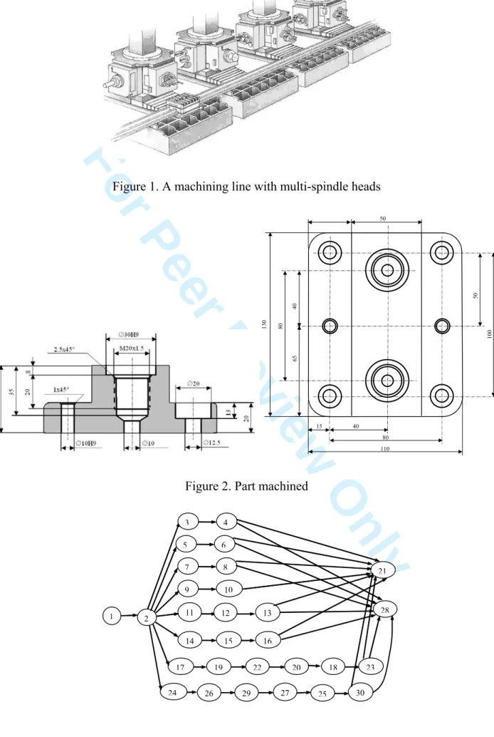
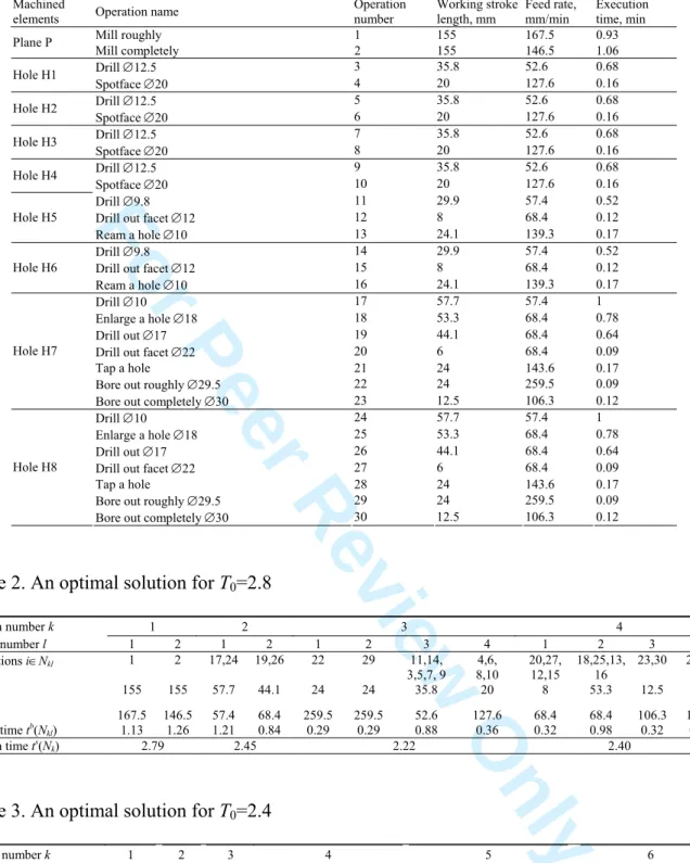
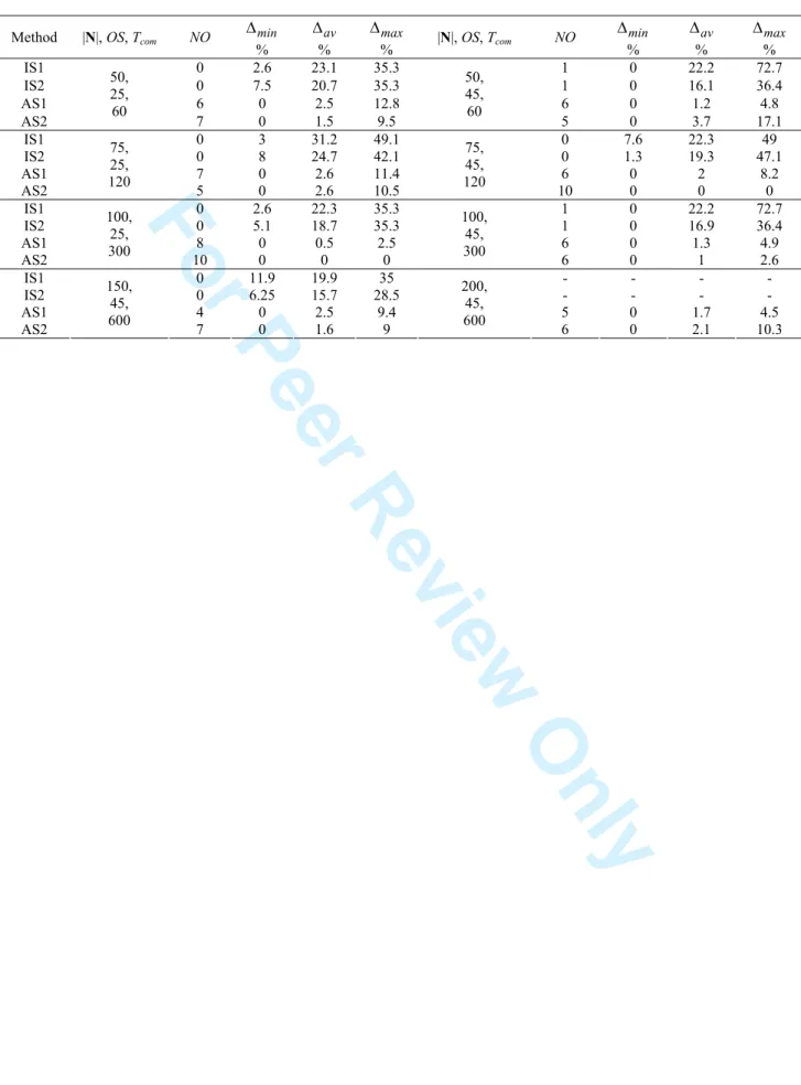
Figure
Documents relatifs
All groups considered in this paper are abelian and additively writ- ten ; rings are associative and with an identity, modules are unitary... The
On the way, we give an alternative proof of Moussong’s hyperbolicity criterion [Mou88] for Coxeter groups built on Danciger–Guéritaud–Kassel [DGK17] and find examples of Coxeter
Suppose now that theorem 3 is valid for codimension q — 1 foliations and let ^ be a ^codimension q strong ^-foliation on X given by the equation a? 1 = 0,. , c^ are closed Pfaff
In [13], Ray introduced Q-balancing matrix and using matrix algebra he obtained several interesting results on sequence of balancing numbers and its related numbers sequences..
On Figure 4 we can visual- ize the proportion of homonyms when drawing from the French population in Paris, either drawing pairs or drawing first and last-names independently..
(I have to thank G. 111 gives in mostcases a degree, which is divisible by p, butnota power of p.. Then G has the degree 21.. Hence by lemma 4 of partI we can assume thatG/N is
In this paper, we consider the related class X of groups G which contain proper nonabelian subgroups, all of which are isomorphic to G.. Clearly, every X-group
- In case of very different sclare measures between the variables, it is better to use the normalized Euclidean distance to give all the variables the same weight.. Note that this
