HAL Id: tel-02085091
https://tel.archives-ouvertes.fr/tel-02085091v2
Submitted on 27 Apr 2021HAL is a multi-disciplinary open access archive for the deposit and dissemination of sci-entific research documents, whether they are pub-lished or not. The documents may come from
L’archive ouverte pluridisciplinaire HAL, est destinée au dépôt et à la diffusion de documents scientifiques de niveau recherche, publiés ou non, émanant des établissements d’enseignement et de
Jean-Benoît Griesner
To cite this version:
Jean-Benoît Griesner. Scalable models for points-of-interest recommender systems. Information Re-trieval [cs.IR]. Télécom ParisTech, 2018. English. �NNT : 2018ENST0037�. �tel-02085091v2�
T
H
È
S
E
EDITE - ED 130Doctorat ParisTech
T H È S E
pour obtenir le grade de docteur délivré par
TÉLÉCOM ParisTech
Spécialité « Informatique »
présentée et soutenue publiquement par
Jean-Benoît Griesner
le 3 Juillet 2018
Systèmes de recommandation de POI à large échelle
Directeurs de thèse: Talel Abdessalem et Hubert Naacke
Jury
M. Talel Abdessalem, Professeur, Télécom ParisTech Directeur de thèse Mme. Florence d’Alché-Buc, Professeur, Télécom ParisTech Examinatrice M. Stéphane Bressan, Professeur associé, National University of Singapore Rapporteur M. Amin Mantrach, Directeur de Recherches, Criteo Labs Rapporteur M. Hubert Naacke, Maître de Conférences, Université Pierre et Marie Curie Directeur de thèse M. Fabrice Rossi, Professeur, Université Paris 1 Panthéon-Sorbonne Examinateur
The task of points-of-interest (POI) recommendations has become an essential feature in location-based social networks. However it remains a challenging problem because of specific constraints of these networks. In this thesis I investigate new approaches to solve the personalized POI recommendation problem. Three main contributions are proposed in this work.
The first contribution is a new matrix factorization model that integrates ge-ographical and temporal influences. This model is based on a specific processing of geographical data. The second contribution is an innovative solution against the implicit feedback problem. This problem corresponds to the difficulty to dis-tinguish among unvisited POI the actual "unknown" from the "negative" ones. Finally the third contribution of this thesis is a new method to generate recom-mendations with large-scale datasets. In this approach I propose to combine a new geographical clustering algorithm with users’ implicit social influences in order to define local and global mobility scales.
La recommandation de points d’intérêts (POI) est une composante essentielle des réseaux sociaux géolocalisés. Cette tâche pose de nouveaux défis dûs aux con-traintes spécifiques de ces réseaux. Cette thèse étudie de nouvelles solutions au problème de la recommandation personnalisée de POI. Trois contributions sont proposées dans ce travail.
La première contribution est un nouveau modèle de factorisation de matrices qui intègre les influences géographique et temporelle. Ce modèle s’appuie sur un traitement spécifique des données. La deuxième contribution est une nouvelle solu-tion au problème dit du feedback implicite. Ce problème correspond à la difficulté à distinguer parmi les POI non visités, les POI dont l’utilisateur ignore l’existence des POI qui ne l’intéressent pas. Enfin la troisième contribution de cette thèse est une méthode pour générer des recommandations à large échelle. Cette ap-proche combine un algorithme de clustering géographique avec l’influence sociale des utilisateurs à différentes échelles de mobilité.
L’épilogue de mon doctorat approche. Cette perspective me conduit à remercier chaleureusement toutes les personnes qui ont rendu possible cette aventure, certes trop rapide, et sans lesquelles ces trois dernières années n’auraient pas eu la même saveur. Qu’elles reçoivent ici l’assurance de ma sincère reconnaissance.
Je voudrais en première intention témoigner toute ma gratitude à mes deux di-recteurs de thèse, Messieurs Talel Abdessalem et Hubert Naacke, pour leur soutien inconditionnel. Ils ont su me guider avec pertinence et bienveillance et orienter à bon escient mes recherches. Sans leur aide et leurs conseils éclairés l’écriture de cette thèse n’aurait sans doute pas été achevée.
J’exprime également mes remerciements à Messieurs Stéphane Bressan et Amin Mantrach, rapporteurs de ce manuscrit, ainsi qu’aux autres membres de mon jury de soutenance, Madame Florence d’Alché-Buc et Monsieur Fabrice Rossi, pour leur disponibilité et leurs nombreux avis.
J’ai bien conscience d’avoir eu l’opportunité de bénéficier à Télécom ParisTech d’un environnement propice et stimulant. Je remercie à cet égard chaque membre de l’équipe DBWeb pour les incessantes réflexions partagées et les amicales discus-sions.
Enfin j’adresse à mes parents Patrick et Annie et à mon frère Jean-Baptiste mes pensées les plus aimantes et affectionnées.
1 Introduction 15
1.1 Research Motivation . . . 15
1.2 Points-Of-Interest and Social Networks. . . 18
1.3 General Objectives . . . 19
1.4 Research Goals . . . 20
1.5 Contributions . . . 21
1.6 General Definitions. . . 22
1.7 Structure of the Thesis . . . 25
2 A Survey on Points-Of-Interest Recommender Systems 27 2.1 A Recommender Systems Overview . . . 27
2.1.1 Background. . . 28 2.1.2 Algorithms Classification. . . 30 2.1.3 Challenges . . . 37 2.1.4 Evaluation . . . 38 2.2 POI Recommendation . . . 40 2.2.1 Problem Definition. . . 40
2.2.2 Different POI Recommendation Problems . . . 41
2.2.3 Hybrid Collaborative Filtering Models. . . 42
2.2.4 Graph Based Approaches . . . 43
2.2.5 Matrix Factorization Models . . . 44
2.3 Overview of Important Models. . . 46
2.3.1 Existing Methods . . . 46
2.3.2 Models of this Thesis . . . 46
3 An Efficient Matrix Factorization Model for POI Recommenda-tion 49 3.1 Introduction . . . 49
3.2 Related Matrix Factorization Models . . . 51
3.5 Experiments. . . 55
3.5.1 Dataset and Experimental Setup . . . 55
3.5.2 Evaluation Metrics . . . 56
3.5.3 Results and Discussions . . . 57
3.6 Conclusions . . . 57
4 A Factorization Based Solution to the Implicit Feedback Problem 61 4.1 Introduction . . . 61
4.2 Existing Implicit Feedback Approaches. . . 63
4.3 A Factorization Model for Implicit Feedback . . . 65
4.4 GeoSPF: Modeling Geographical and Social Influences . . . 66
4.4.1 General Idea . . . 66
4.4.2 Geographical Accessibility . . . 69
4.4.3 AGRA: Accessibility Graph . . . 70
4.4.4 GeoSPF: An Implicit Social Factorization. . . 71
4.4.5 Inference . . . 74
4.5 Experimental Evaluation . . . 75
4.5.1 Data Sets and Metrics Description . . . 75
4.5.2 Comparison with competitor models . . . 76
4.6 Conclusion. . . 79
5 ALGeoSPF: A Clustering Based Factorization Model for Large Scale POI Recommendation 81 5.1 Introduction . . . 82
5.1.1 Contributions . . . 82
5.1.2 Road Map . . . 84
5.2 POI Recommendation at Large Scale . . . 84
5.3 ALGeoSPF: Local-Global Spatial Influence Modeling . . . 85
5.3.1 General Idea . . . 85
5.3.2 Super-POIs . . . 86
5.3.3 Mobility Behaviors . . . 87
5.3.4 Final Objective . . . 88
5.4 Hierachical SuperPOIs Layers . . . 89
5.4.1 Geographical Clustering Algorithm. . . 90
5.4.2 Personalized Class Selection . . . 91
5.5 Experimental Evaluation . . . 93
6 Conclusion 99
6.1 Summary . . . 99
6.2 Outlook . . . 100
A Résumé en français 103 A.1 Introduction . . . 104
A.2 Axes de recherche . . . 105
A.3 Contributions . . . 106
A.4 GeoMF-TD : Un modèle de factorisation de matrices pour la recom-mandation de POI . . . 107
A.4.1 Factorisation de matrices géographique . . . 108
A.4.2 GeoMF avec dépendances temporelles . . . 110
A.4.3 Résultats expérimentaux . . . 111
A.4.4 Conclusions . . . 112
A.5 GeoSPF : influences sociales implicites . . . 112
A.5.1 Factorisation de Poisson et feedback implicite . . . 113
A.5.2 Modèle d’influence sociale . . . 113
A.5.3 Résultats expérimentaux . . . 118
A.5.4 Conclusion . . . 121
A.6 Passage à l’échelle avec ALGeoSPF . . . 122
A.6.1 Idée générale . . . 122
A.6.2 Hiérarchie de superPOI. . . 124
A.6.3 Résultats expérimentaux . . . 125
A.6.4 Conclusion . . . 126
1.1 The POI search engine of https://foursquare.com/. . . 16
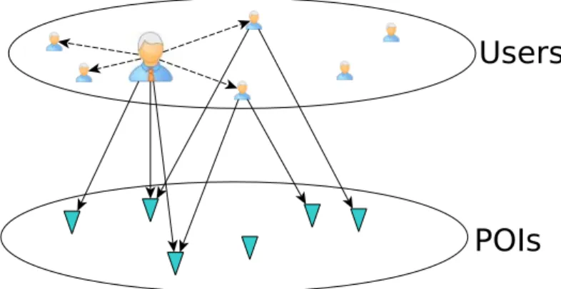
1.2 Three layers of the information layout in LBSNs. . . 19
1.3 Standard Location-based Social Network Components. . . 23
3.1 Check-in distribution from Gowalla users during 21 months of the most visited POIs in France. . . 56
3.2 Precision comparison between GeoMF and GeoMF-TD . . . 58
3.3 Recall comparison between GeoMF and GeoMF-TD. . . 58
4.1 An illustration of a user’s social network and the check-ins of her friends. GeoSPF is based on the central idea that the target user should benefit from the visit experiences of her friends. Her social network is extracted through the geographical mobility patterns ob-served in the data. Then our approach integrates her friends’ existing check-ins into a factorization model. . . 67
4.2 Density of inter check-ins distances distribution on 4 datasets.. . . . 68
4.3 Density of inter check-ins accessibilities distribution on 4 datasets. . 70
4.4 Performance results of 4 Methods on Gowalla. Each figure represents the performance results of the four metrics described in section 4.4 for a different number of edges in the graph. This number of edges is controlled by the average social graph degree. . . 72
4.5 Graphical model of our approach. . . 74
4.6 European YFCC dataset. . . 75
4.7 Performance comparison w.r.t. state-of-the-art approaches for three datasets: Foursquare, Gowalla@Paris and Gowlla. We plot Re-call@N for N=5 and N=10 on Figures A.4a, A.4b and A.4c. We plot NDCG@5 on figure A.4d. We observe that GeoSPF outperforms sig-nificantly baselines on the three datasets for the three performance measures. . . 78
users and for different values of Nmaxand three different geographical
areas: Europe, France and Paris. We observe that each user has a peak of density depending on an optimal Nmax which characterizes
the class of the user. . . 92
5.3 Performance comparison of ALGeoSPF wrt. state-of-the-art ap-proaches for 2 levels of the YFCC dataset. We plot on figure A.5a the recall@10 results of GeoSPF and ALGeoSPF for different size of the average social graph degree. Figure A.5b presents the results of AMGeoSPF in terms of recall@5 and recall@10. . . 98
A.1 Résultats comparatifs entre GeoMF et GeoMF-TD . . . 112
A.2 Résultats de performance des 4 métriques sur Gowalla. Chaque figure représente les résultats de performance des quatre mesures décrites dans la section A.5 pour un nombre différent d’arêtes dans le graphique. Ce nombre d’arêtes est contrôlé par le degré moyen du graphe social. . . 116
A.3 Modèle graphique de GeoSPF. . . 118
A.4 Comparaison des performances avec des approches alternatives pour trois jeux de données : Foursquare, Gowalla@Paris et Gowlla. Nous traçons le Recall@N pour N = 5 et N = 10 sur les figures A.4a, A.4b et A.4c. Nous traçons le NDCG@5 sur la figure A.4d. Nous observons que GeoSPF dépasse de manière significative les autres modèles sur les trois jeux de données pour les trois mesures de qualité choisis. . . 120
A.5 Performance comparison of ALGeoSPF wrt. state-of-the-art ap-proaches for 2 levels of the YFCC dataset. We plot on figure A.5a the recall@10 results of GeoSPF and ALGeoSPF for different size of the average social graph degree. Figure A.5b presents the results of AMGeoSPF in terms of recall@5 and recall@10. . . 126
1.1 An example of a points-of-interest and its associated information . . 17
1.2 Table of Notations . . . 24
2.1 Illustration of a users’ rating matrix X. . . 29
2.2 Collaborative filtering classes: advantages & shortcomings.. . . 35
2.3 Overview of some recent points-of-interest recommendation techniques. 47
3.1 Statistics of the Gowalla data set . . . 55
4.1 Statistics on the datasets . . . 76
5.1 Statistics on the datasets . . . 94
A.1 Statistiques sur le jeu de données issu du LBSN Gowalla utilisé dans les expériences. . . 111
Introduction
We propose in this thesis new efficient methods in order to recommend personalized and relevant points-of-interest to users. To this end, this first chapter is aimed at proposing a global overview of the work carried out throughout this thesis. In particular we describe our research motivation in Section 1.1. Some first definitions come in Section 1.2. Then we describe our general objective in Section1.3 and our research goals in Section 1.4. We present the contributions that we achieved in Section 1.5. Finally we present briefly the structure of the thesis in Section 1.7.
1.1
Research Motivation
The development of the Web 2.0 [Lewis 2006] these last years has promoted the emergence of a large number of LocatiBased Social Networks (LBSNs) or on-line networks with location-based features such as Twitter, Facebook, Google+, Foursquare, Flickr and so on, which have changed deeply our vision of our environ-ment and how we interact with it. A LBSN is a special category of online social network [Klein, Ahlf, and Sharma 2015] whose its content is directly associated to our geographical world. As a consequence geography and locations have both a crucial impact first on LBSNs structure and also on the quality of the services provided to the users and on the way their personal data are processed. Indeed LBSNs propose many different location-based services to their users ranging from transport to weather and news or recommendation services for instance. These ser-vices are especially interesting for the user facing a new or unknown environment. As a result these networks have developed more and more technologies, services and supports to help their users who want to explore and discover this unknown environment. Moreover users are now so used to interact with these online services that a new information need has emerged. Due to this information need and thanks
Figure 1.1: The POI search engine ofhttps://foursquare.com/.
to these new services LBSNs constitute nowadays the most abundant sources of available information related to the global users’ preferences, habits and activities [Chorley, Whitaker, and Allen 2015].
Indeed the amount of personal information and resources shared on these LB-SNs has risen exponentially these last years [Cui, Hero, Luo, and Moura 2016]. For instance on the LBSN Flickr1 there are more than 110 millions users who produce
more than one million images per day. Because of this information overload [Toffler 1970], it has become increasingly difficult for the users to find what they are look-ing for in their surroundlook-ings. For instance it is common for a user who is looklook-ing online for a restaurant abroad to be overwhelmed by the intractable quantity of information to consider. As a consequence different POI search engines have been developed these last years to meet this need. An example of such a POI search engine can be seen on Figure 1.1.
To address this information overload problem, Recommender Systems (RS) have become an essential technology. The recommender systems most general purpose is to provide a personalized assistance to the users who require help for searching, ranking or filtering the large amount of information available on LBSNs. More preciselly the main goal of recommender systems [Adomavicius and Tuzhilin 2005] is to propose to users personalized recommendations that are useful to dis-cover interesting and new items that users would have probably not disdis-covered on their own. These systems are now widely adopted by online business platforms in varied contexts ranging from books (Amazon2), movies (Netflix3), music (Spotify4)
or Points-Of-Interest (POIs) with applications such as Foursquare5. As said
previ-ously, these platforms are usually characterized by the large spaces of shared data they manage: 500 million messages exchanged everyday on Twitter by 248 million
1 https://www.flickr.com/ 2https://www.amazon.com/ 3 https://www.netflix.com/fr/ 4 https://www.spotify.com/fr/ 5 https://fr.foursquare.com/
users, 200 million products in Amazon, 30 million songs in Spotify, 10,000 movies in Netflix... Such volumes of candidate items to explore impose harsh practical limitations for the user who wants to filter, search or select the interesting online information. Indeed without an efficient online assistant it becomes impossible for the user to navigate in these large spaces. As a consequence the importance to pro-pose highly accurate recommendation lists and efficient filtering tools has become a major issue in this context.
Many recommendation problems have been investigated these last years in a large number of topics and domains, ranging from music recommendation [Cheng, Shen, and Mei 2014] to news recommendation [Hsieh et al. 2016] and movies rec-ommendation [Gantner, Rendle, and Schmidt-Thieme 2010]. As a result one might expect that it exists now a large number of models and approaches to solve most of recommendation difficulties. However the problem of points-of-interest recom-mendation involves several specific challenges that distinguish it from traditional recommendation tasks (such as books, music or movies...) especially because of geographical influence, side information, user mobility and implicit user feedback. In this thesis we address such recommendation-specific challenges. More precisely we investigate the impact of these challenges on the recommendation quality and we propose new approaches to solve them.
point-of-interest name Eiffel Tower #Checkins 7.097.302
Location Latitude: 48.858° Longitude: N, 2.294° E Categories scenic views, monument, entertainment, leisure Table 1.1: An example of a points-of-interest and its associated information
Motivated by these specific constraints and challenges, the problem of geograph-ical items recommendation and specifgeograph-ically the problem of POI recommenda-tion has received an increasing level of interest in the academic world in the last years [Jing, Xin, and Lejian 2017]. Therefore a large number of works have been proposed to address this problem these last years. Existing works span from the industry to the academic world, especially in top tier conferences in computer sci-ence such as ACM RecSys [Baral and Li 2016], KDD [Li, Ge, Hong, and Zhu 2016], WWW [Ying, Chen, Xiong, and Wu 2016], CIKM [Xie et al. 2016], IJCAI [Jing, Xin, and Lejian 2017], SIGIR [Yuan, Cong, Ma, et al. 2013] and many more. All these approaches aim at combining different existing layers of information into one recommendation model. However the information layers contain complex objects
existing model.
1.2
Points-Of-Interest and Social Networks
A point-of-interest6 is a uniquely identified specific site generally associated to a
specific category of activities (e.g. museum, restaurant, university etc.). Similarly to checkins (defined below) in LBSNs a point-of-interest is generally also associated with some content which corresponds to the set of all comments, pictures, opinions that users have uploaded during the checkins they made. For instance in table 1.1
the point-of-interest Eiffel Tower is associated with some of the categories it be-longs to. However in many practical cases the categories or other point-of-interest descriptions are not disclosed for various reasons (e.g. privacy, confidentiality etc.). This is why in our approaches we have assumed that we only know the locations, i.e. the pairs (latitude, longitude) for all points-of-interest.
On the other hand the checkins correspond to the visits made by users in points-of-interest. Therefore checkins are always associated at least with a POI and a location (i.e. a pair {longitude, latitude}) and a date (e.g. a timestamp). These information are required to deal with geographical and temporal dimensions. Checkins can also be associated to different content. However taking into account of these metadata requires more complex input models, which eventually increases the training duration and the computational complexity of the recommendation model. We propose on figure1.2 an overview of the standard structure of a LBSN. On this figure we distinguish three main layers: first the map and the points-of-interest (i.e. the geographical layer or the physical layer), then the users (i.e. the so-cial layer) and finally the content shared online by the users (i.e. the content layer). The information contained by these layers come with specific constraints and characteristics that are likely to influence the final quality of the models and that require to be taken into account. For instance it has been demonstrated that the geographical layer content has the most significant impact on the recommen-dation final quality [Lian et al. 2014]. As a result it is necessary to consider how to exploit all the layers in order to increase the efficiency of our recommendation models. Unfortunately the information contained by the content layer are often not disclosed for privacy purpose. Moreover it does not exist any universal method to manage these data. For these reasons we will not exploit the content layer
Figure 1.2: Three layers of the information layout in LBSNs. information directly in this thesis.
1.3
General Objectives
The general objectives of this thesis are twofold. First we investigate and propose new matrix factorization methods to address the POI recommendation problem based on LBSN data. Actually existing matrix factorization methods are not de-signed to integrate the items locations directly into their models, which results in a poor recommendation quality. Especially we consider that the improvement in terms of ”quality” of recommendations has to take into account of how users ex-plore their surroundings and what are their specific mobility patterns. The quality of the recommendation7 can be defined either in terms of ranking or in terms of
prediction. The prediction quality aims at generating a recommendation score that reflects directly the preference of a given user for a given POI. In this case the score is an estimation of to which extent the user appreciates a given POI. On the other hand the ranking quality aims at optimizing the ranking of points-of-interest for a given target user. In the case of ranking the computed score gives only a possibility to sort the top-k list recommended.
Our second objective is to address the problem of scalability of such methods. Indeed, as said briefly in the previous section, most of recommendation algorithms
large number of points-of-interest which makes the recommendation models inef-ficient. For instance most of factorization methods have a quadratic complexity [Hu, Koren, and Volinsky 2008]. The other issue of scalability is due to the large geographical target area that increases significantly the complexity to explore all possible points-of-interest in this area. As a result our goal is to adapt these models and also to investigate new techniques to compute efficient models on very large volume of data such as the YFCC dataset proposed by [Thomee et al. 2016].
1.4
Research Goals
The most general objective of this thesis, as described above, is to improve the quality and the scalability of POI recommendation approaches based on LBSN data. To do this we have been led to pursue the following research goals (or RG): RG n°1: Survey of existing methods regarding point-of-interest rec-ommendation. As described in the previous sections, it exists in the related work a large number of methods and models for POI recommendation. However a clear understanding of the effective advantages and shortcomings between these models is still missing. Therefore we inspect and propose a complete panorama of the most efficient techniques and approaches (c.f. Section 2).
RG n°2: Explore and improve matrix factorization approaches. Since the Netflix Prize [Bennett, Lanning, and Netflix 2007] we know that factorization approaches are the most efficient among collaborative filtering methods to face sparsity issues. So we investigate factorization methods in order to connect them with specificities of point-of-interest recommendation. In particular the goal here is to integrate geographical and temporal influences.
RG n°3: Investigate the probabilistic framework for factorization models. Probabilistic rules and assumptions allow to build more flexible and efficient methods that allow to enhance the quality of the model. Therefore we propose new probabilistic approaches to better take into account of sparsity issue and contextual information as well.
RG n°4: Enhance scalability of factorization approaches. Most point-of-interest recommendation techniques fail to handle large volumes of users and POI. As a result most of existing experimental datasets used to test in literature
are several order of magnitude smaller than real-world datasets. This is why we aim at exploring possible solutions to alleviate this issue. We investigate especially geographical clustering methods to tackle the sparsity and the scalability problems. RG n°5: Explore geographical users’ mobility patterns. LBSN pro-vide a rich and precise source of information regarding users habits. This source of information can be exploited to enhance our understanding of the geographical mobility patterns of users. More precisely we exploit the observation of different scales of mobility: some users tend to travel through the whole world, on long distance, while others will concentrate their checkins in local areas.
1.5
Contributions
The work conducted throughout this thesis has resulted in several achievements in the area of POI recommendation. This section describes briefly our main contri-butions.
Contribution n°1: A geographical matrix factorization model with time dependencies: GeoMF-TD. We have proposed a factorization model that takes into account of the spatio-temporal distributions of checkins in the data. GeoMF-TD divides the given target region in a grid of even cells. This grid is exploited then to model the geographical and temporal latent influences of POI and users’ activity through the cells of the grid. These latent influences are then combined linearly with latent vectors to compute the recommendation score. We have proposed such a new model in [Griesner, Abdessalem, and Naacke 2015]
Contribution n°2: GeoSPF, an approach to the implicit feedback problem based on a Poisson factorization model. Poisson factorization has been exploited successfully for various recommendation problems. Based on a Poisson factorization model, we have enhanced the contextual information influ-ence by building an implicit social network. This implicit social network is based on geographical preferences of users. We have investigated this line of research in [Griesner, Abdesssalem, and Naacke 2017]
Contribution n°3: A new model for users’ personal geographical mo-bility patterns. We usually observe in LBSN datasets different user profiles: some users tend to make long distance trips whereas other users only do checkins limited to a local area. We have exploited this observation to face the scalability issue by
Contribution n°4: ALGeoSPF, a large-scale extension of GeoSPF. Based on previous contributions we have proposed a new approach that can build personalized POI recommendations on large-scale datasets. This work has resulted in our ALGeoSPF model. We have presented this work in [Griesner, Abdesssalem, Naacke, and Dosne 2018].
1.6
General Definitions
In this section we give the main definitions of terms and expressions used through-out this thesis. A list of notations used in the following is also proposed in Table
1.2 below. We define first what a point-of-interest is:
Definition 1.6.1. (Point-of-Interest) A point-of-interest is a uniquely identified specific site associated to a specific activity (e.g. museum, restaurant, university...). In LBSN a POI is generally also associated with some content. For instance in table 1.1 the POI is associated with some of the categories it belongs to. However in many practical cases the categories or other POI descriptions are not disclosed for various reasons (e.g. privacy). In our thesis we assume that we only know the location, i.e. the pair (latitude, longitude) of every POI. Because of this reason in this thesis the terms point-of-interest, location, spot, place, site can designate indifferently the same thing. In the same way we can define the check-ins made by users into points-of-interest as follows:
Definition 1.6.2. (Check-in) The check-in activity of a user u visiting a POI p at a time t is a tuple < u, p, t >.
To compute the visit frequency of u in p we count how many corresponding check-ins have been made. Given that in our approach each POI is associated with at least one super-POI, each check-in of a POI increments the corresponding super-POI visit frequency. We draw on figure 1.3 a standard representation of an LBSN with points-of-interest and check-ins. We observe that most of LBSNs have in common the following data attributes: a user setU, a POIs set P, some temporal information T and a social network S.
In this framework, basically, a user u can make a check-in at some POI p at a time t. These check-ins constitute the user profile of the user as defined below:
Definition 1.6.3. (User Profile) A user profile is the set of all the check-ins that the user made in the past: Pu = {< u, p
i, tj > / < u, pi, tj >∈ D}. Each user
is associated to her profile. The aggregation of all user profiles constitutes the full dataset D = {Pu/u ∈ U}. The user profile can also be defined as a set of check-ins
sequences. A sequence of check-ins that the users made between a K number of consecutive points-of-interest can be noted as follows: {p1→ p2 → ... → pk/p ∈ P}.
We propose now to define more the specific recommendation problem that this thesis aims at solving. For a given set of points-of-interest: P = {p1, ..., pm}
and for a given set of users: U = {u1, ..., un}, each user is associated with a
chronologically ordered set of points-of-interest Lu visited by the user u such that
Lu= {p1
u→ p2u → ... → pku} where k = ∣Lu∣, we define the problem of points-of-interest
recommendation:
Definition 1.6.4. (Points-of-interest recommendation problem) is the prob-lem of recommending for any user u∈ U a top-k list ˆLu of new unvisited
points-of-interest, that is to say points-of-interest that belong to the set P ∖ Lu, that are the
most likely to match the user preferences and thus to be visited by u.
We can distinguish two main cases8. Indeed we say that the recommendation
can be either generic if the system proposes points-of-interest without considering the given user, i.e. recommends the same list for any user as follows: ∀u, ˆLu= ˆLGen
On the other hand the recommendation is said personalized if the recommendation result depends effectively on the user, as follows: i.e. ∀u, ˆLu = ˆLP ers[u]. Generic
techniques allow the recommender system to produce recommendation for a large variety of different items: they are called domain independent. On the counterpart they perform usually poorly because of the lack of contextual information. On
8These cases are described in Chapter2
U Set of all users {u1, u2, ..., u∣U ∣}
P Set of all POIs {p1, p2, ..., p∣P ∣}
P Family of all layers of super-POIs: P= ⋃kPk
Pu, Eu Sets of POIs and edges visited by user u
< u, p, t > Check-in of user u visiting POI p at time t D Collection of all check-ins of all users
visiting all POIs: D = {< ui, pi, ti>} ∣D∣ i=1
Tj,j+1 Transition probability betwen POIs j and j+ 1
Aj,j+1 Accessibility between POIs j and j+ 1
G Geographical accessibility digraph G= (V, E, ρ) Γ(X) Set of POIs accessible in one hop from X
Γ(X) = {p′∈ V ∣p ∈ X ∧ A
p,p′ > 0}
X= [xup] The ∣U∣ × ∣P∣ user-POI check-in matrix
xup Visit frequency of user u in POI p
yup Recommendation score of POI p for user u
ui Vector of Rm×k user latent factors
vj Vector of Rn×k POI latent factors
the other hand, personalized techniques result in a better final quality, but require more complex models.
Based on this definition we could consider two specific instances of the point-of-interest recommendation problem. The first one is a user that has made all her checkins in a given city C. Consequently her associated history list Lu contains
only points-of-interest close from each other. For this user the recommendation model has to deduce what is the maximum distance that the user could accept for visiting a relevant POI: if the relevant POI is too far away, the user will probably not visit it.
Reciprocally the second instance is a user who made checkins in a wide geo-graphical area (e.g. on all continents). We claim that for this user the distance will not be a serious constraint. However we could face a scalability issue given that more points-of-interest will have to be considered. We observe here that an efficient recommendation model has to detect these two patterns and adapt its parameters to the target user.
1.7
Structure of the Thesis
We have structured our thesis as follows.
• Chapter 1 introduces our thesis. That is to say it presents the research motivation of our problem, the general objectives we want to complete, the contributions that we achieved and general definitions used throughout this thesis.
• Chapter 2 proposes first a global overview of the recommendation concept and process. Then the second part of this chapter is dedicated to a specific introduction to points-of-interest recommendation. Finally it concludes by describing the position of the techniques proposed in our work among the related works.
• Chapter 3 dives into our geographical matrix factorization model named GeoMF-TD. We present its structure and main ideas.
• Chapter4introduces geoSPF, our Poisson-based factorization approach that integrates geographical and social influences.
• Chapter 5 presents ALGeoSPF, an extension of GeoSPF that takes into ac-count of the specific mobility patterns of the users in a personalized way. • Chapter6contains the conclusion that we reached throughout this thesis and
A Survey on Points-Of-Interest
Recommender Systems
Investigating the related work in areas regarding the problem of Points-Of-Interest (POI1) Recommender Systems (RS) represents an essential part of the work that
has been conducted in this thesis. Our purpose is to present a comprehensive and systematic exploration of algorithms and ideas from this field. Thus in this chapter we propose a review of main existing approaches and technologies. Specifically we have investigated works linked to geographical, social and temporal influences for POI RS. In particular we propose a global classification of main existing POI rec-ommendation algorithms. We start by defining the general recrec-ommendation process in Section 2.1. Then we delve into the specificities of POI recommendation in Sec-tion 2.2. Finally we propose an overview of the models we propose in this thesis in Section 2.3.
2.1
A Recommender Systems Overview
The most general goal of a recommender system (also noted RS) is to suggest to online users items to consume or to select [Adomavicius and Tuzhilin 2005]. Most of the time these items are expected to be new or at least that she could not find on her own. Furthermore these items are also expected to match the user preferences and so to contribute positively to the user experience. This is why these systems propose to the user a personalized exploration of a large space of possible choices. Differently from pure information retrieval systems where the user navigates into this possible space of choices by expressing an explicit query, the RS is not aware ”a priori” of what the user really wants or prefers. In other words in a standard
recommendation scenario the RS have to infer the implicit personal information needs of the users. As a consequence, because there is no explicit query, the RS can only exploit all past interactions of the user with the system to generate recom-mendations. This is why recommender systems collect and analyse all past user’s preferences in order to predict future preferences.
Moreover, from a business point of view the RS goal is to transform a standard user into a consumer. The business value here is to increase the conversion rate of the POIs owner [Ricci, Rokach, Shapira, and Kantor 2010]. This task is com-pleted especially by enhancing the loyalty of the user to the system, which is done by improving her browsing experience. Thus the recommender systems business purpose is to improve the quality of the users’ interaction with the system, and to help the user through a large space of possible relevant items to select and consume. In this Chapter we provide an introduction to the recommendation scenario from a technical point of view. The first part of this introduction is mainly based on many exhaustive state-of-the-art studies and surveys in the field of recommen-dation, such as [Borris, Moreno, and Valls 2014; Barbieri, Manco, and Ritacco 2014] and many others. The second part of the introduction is mainly based on POI recommendation surveys. First, we provide in subsection 2.1.1 a formal back-ground that introduces some notations used in the sequel. We present a brief classification of existing recommendation algorithms in subsection 2.1.2. Then we will discuss the challenges and evaluation involved by RS in subsections 2.1.3 and
2.1.4 respectively.
2.1.1
Background
As said in the introduction, recommender systems are tools that are used to lead the users to the items they prefer without asking any question [Adomavicius and Tuzhilin 2005]. More formally a recommender system generates to users personal-ized lists of K items as close as possible to the users’ preferences. Modelling this recommendation scenario requires obviously, at least, three entities: users, items and preferences. Any other contextual entities or information related to the users or items can then be integrated a posteriori into the model. In the following we present some of the notations that we use in the sequel of this thesis to model these entities.
As said above, any recommendation scenario involves at least users and items. So let U = {u1, ..., uM} be a set of M users and let I = {i1, ..., iN} be a set of N
i1 i2 i3 i4 i5 i6 i7 i8 i9 i10 u1 3 1 4 u2 5 2 2 u3 1 2 4 2 1 4 u4 3 4 2 u5 1 5 u6 2 1 5 1 u7 4 2 1
Table 2.1: Illustration of a users’ rating matrix X.
items. For sake of clarity we traditionnally represent the users’ preferences in a M × N matrix X = [xui] ∈ SM ×N. This is why we define X the user-item rating
matrix. The set S is the set that contains all possible values for elements xui of
X. In X the element xui represents the preference value of the user u for the item
i. The set S is called the domain of scores and it can contain different types of scores: either bounded ratings (e.g. S = [1, 2, 3, 4, 5]), or only two elements (e.g. S= {like, dislike}), or in the case of behavior data simply frequencies of interactions: S= N+ for instance. We propose an illustration of a possible rating matrix on table
2.1. In this example the scenario involves 7 users, 10 items and explicit preferences ordered from degree 1 to 5. Depending on the meaning associated to values in X, this preference can be classified either as explicit, either as implicit.
• Explicit data corresponds to explicit ratings expressed by the users about the corresponding items. Most of the time these explicit ratings are gathered by asking directly to users their feedback regarding items they have consumed or interacted with in the past [Towle and Quinn 2000]. Then this feedback is converted into explicit preferences. This kind of preferences are more difficult to collect since it requires the user availability. On the counterpart they are easier to interpret than implicit data.
• On the other hand implicit data corresponds to raw observations of the dyads (u, i) in the dataset. We can view these implicit data as a behavioral information that has been recorded only by observing and collecting all past interactions between the users and the system, without asking directly the user’s feedback [Oard and Kim 1998]. For example these behavioral infor-mation can be clicks in a browser, music listened, web sessions, events or check-in in POI. In this case it implies that the entry xui is a nothing more
denotes that u has effectively purchased i.
Behavioral - implicit - data is usually gathered in a silent and passive way, implicit feedback is usually easier to collect than explicit feedback, but it is often unreliable, given that the real effective users’ evaluations remain hidden. On the other hand explicit feedback is usually less abundant but more accurate. Let’s observe that explicit feedback can be either positive or negative, while implicit feedback is always positive. Implicit feedback corresponds here to the One-Class Collaborative Filtering problem [Pan et al. 2008].
Regarding the dimensions, usually the number of users M as well as the num-ber of items N are very large [Ricci, Rokach, Shapira, and Kantor 2010] with typi-cally: M >> N. This is why we say that in traditional real-world recommendation scenarios, the user-item rating matrix X is characterized by an extreme sparse-ness, given that users give their feedback for a (very) limited amount of available items. In the following we will note⟨u, i⟩ the list of all dyads in X such that xui> 0.
More formally we usually note IX(u) = {i ∈ I∣ ⟨u, i⟩ ∈ X} the set of items rated
by user u. On the other hand the set UX(i) = {u ∈ U∣ ⟨u, i⟩ ∈ X} will be the set of
users that have selected/consumed the item i. If the context does not allow any ambiguity regarding the matrix X involved, we can simply note I(u) = IX(u) and
U(i) = UX(i). Some users have not done any selection yet, so we note: I(u) = ∅.
Reciprocally we will say that any user u with a rating history, that is to say such that I(u) ≠ ∅, is an active user.
A classical problem appears when either I(u) or U(i) is empty (which means that a new user or a new item has been added to the dataset). We call this situ-ation the cold start problem [Saveski and Mantrach 2014]. Cold start is generally problematic in RS, since these cannot provide suggestions for users or items if there is not a sufficient amount of information. For instance in table 2.1 the item i5 has
not been rated yet by any user. So this item will never be recommended by any RS given that we have not enough information concerning it.
2.1.2
Algorithms Classification
Because of historical reasons [Ricci, Rokach, Shapira, and Kantor 2010], recom-mendations are generally generated by means of filtering or retrieval techniques. The main idea of these classes of approaches is to remove unwanted information from an information stream in the case of information filtering (IF, online), or
from an information database in the case of information retrieval (IR, offline). In the context of recommendation, ”unwanted” information corresponds to the least relevant items for the target user. To this end, IF/IR based recommendation methods exploit the assumption that human interests and preferences are corre-lated. According to this assumption a user is likely to prefer what other similar users have selected in the past. Thus the most intuitive technique is to collect in-formation about user preferences and to explore similarities between users’ profiles, and then to exploit the known preferences of similar users to build a prediction for the target user.
Filtering algorithms can be classified according to multiple criteria [ Adomavi-cius and Tuzhilin 2005] such as the recommendation domain, the type of feedback, the contextual issues... However the most used classification focuses on the ex-ploitation of the interaction between users, items and the system, and distinguishes three classes of algorithms: content-based, collaborative and hybrid that we present in details in the sequel.
Recommendation Algorithms Content-Based Filtering Collaborative Filtering Hybrid Filtering Features Extraction VSM Similarity Measures Memory-based Model-based CB-CF Content-boosted CF Model/Memory CF 2.1.2.1 Content-Based Filtering
Content-based algorithms (CB) try to find a matching between a user’s profile and item attributes. This works in two steps. First the model learns users’ preferences based on what they purchased in the past. This leads to a user’s profile represen-tation. Then the CB model ranks the items that are the most similar to those the user liked in the past [Pazzani and Billsus 2007]. This requires to have a common item representation for all items. Finally the model provides recommendation of unexperienced items based on this ranked list. Usually in CB filtering, item profiles
and user profiles are represented with a description such as a set of keywords or attributes. In the case where items are textual documents for instance, the key-words are simply the regular key-words of the language contained by the documents. As a result the user profile corresponds to the most relevant keywords of the items she purchased in the past. Once the model has learned each profile, the items are ranked according to a similarity function.
Vector Space Model (VSM). Specifically we denote F = {f1, ..., fq} a set of
de-scriptive features (or attributes) for the itemsI. As said previously, these attributes are usually keywords or scalars extracted from the side information associated to each item. Then the features are exploited to associate each item with a features vector representation. These vectors are then projected into an Euclidean space such as Rq which is called the vector space model (VSM) which is a traditional
model in information indexing [Salton, Wong, and Yang 1975]. The recommen-dation score is then derived from a list of candidate items ranked thanks to the similarity function between vectors in the VSM. Let wi ∈ Rq be the feature vector
associated with item i∈ I. Each component wf
i represents the contribution weight
of feature f for the item. The values wf
i can be either binary, categorical or
nu-merical depending on the data specifications.
TF-IDF. One of the most used method [Ricci, Rokach, Shapira, and Kantor 2010] to build these weights is the TF-IDF method, that gives for a given document D more importance to terms that appear frequently (TF≡Term Frequency), but also that penalizes terms that occur frequently in other documents (IDF≡Inverse Document Frequency). The TF-IDF function is defined as follows:
TF-IDF(tk, dj) = freqk,j maxzfreqz,j ´¹¹¹¹¹¹¹¹¹¹¹¹¹¹¹¹¹¹¹¹¹¹¹¹¹¹¹¸¹¹¹¹¹¹¹¹¹¹¹¹¹¹¹¹¹¹¹¹¹¹¹¹¹¹¹¶ T F ⋅ log(nN k) ´¹¹¹¹¹¹¹¹¹¹¹¸¹¹¹¹¹¹¹¹¹¹¹¹¶ IDF (2.1)
where tkis the target term, dj the target document, N is the number of documents
in the corpus, nkthe number of documents containing the term tk and freqk,j refers
to the frequency of term tk in document dj.
Once the items have a representation in the VSM, one can either apply machine learning techniques, or directly similarity function. For a given user’s profile, the main idea is to classify items in two classes: C = {c+, c−} of positive and negative class depending on if the item is relevant or not for the user. Machine learning techniques have been widely exploited by CB approaches. However this is outside of our scope, so we will not present more this topic.
Similarity functions. Given a target user’s profile, similarity functions are nec-essary to determine how relevant two candidate items are. It exists a large choice of possible ways to measure how close two vectors are. The most commonly used similarity functions are the following:
• Minkowski distance: This is a generalization of the notion of distance between two points in an Euclidean space. The distance between items i and j is defined as follows: dM inkp (i, j) = ( q ∑ l=1 ∣wi,l− wj,l∣ p ) 1 p (2.2) • Cosine similarity: It measures the similarity of two items with the angle between their corresponding vectors. This similarity function is especially used with sparse feature vectors. It is defined as follows:
simCos(i, j) = w
T i ⋅ wj
∥wi∥2⋅ ∥wj∥2
(2.3) • Jaccard similarity: This well-known similarity measures how common fea-tures tend to be predominant in the set of feafea-tures. It is defined as follows:
simJ ac(i, j) = w T i ⋅ wj wT i ⋅ wi+ wjT ⋅ wj− wTi ⋅ wj (2.4)
Advantages & Shortcomings. Because they are based only on content informa-tion and because they don’t require any history of past interacinforma-tions. This provides two advantages [Ricci, Rokach, Shapira, and Kantor 2010]. First CB methods guarantees user independence: the recommendation does not require other users information. Also thanks to this, CB methods don’t suffer from the cold-start problem: even for new user or new item it will be possible to make recommenda-tions. Another advantage is the system is more transparent: it is easy to explain the recommendation result based only on other items and not on other users.
On the other hand CB methods suffer from three important limitations. First they can only recommend items similar to those already purchased by the user. That is to say these methods don’t explore the non-similar items, and hence tend to always recommend the same kind of items, without any diversity but with, pos-sibly, a lot of redundancy. Another problem concerns the features extraction. In
the case of textual data, the features are easy and natural to extract. However for complex data this process is not solved easily yet, because of privacy issues for instance. Moreover it is impossible for CB methods to distinguish between distinct items with the same features, while in reality they could have different value for the user. Finally since the Netflix Prize [Bennett, Lanning, and Netflix 2007], it has been demonstrated that CB methods are globally less accurate than collaborative methods [Koren, Bell, and Volinsky 2009].
2.1.2.2 Collaborative Filtering
Differently from CB approaches, collaborative filtering (CF) does not require any description of items. The term collaborative here means [Schafer, Frankowski, Her-locker, and Sen 2007] that CF methods exploit only all users’ past interactions with the system to make recommendations of items selected by the most similar users of the target user. The central assumption is that users who adopted the same behavior in the past will tend to agree also in the future. As a result CF models are naturally much simpler than CB models,because no side information, such as items description, is required. This makes CF methods more general and especially domain independent. Moreover CF methods allow a higher level of privacy, since no personal information is required. Another advantage of CF is that the more feedback the model receives, the more the recommendation will be accurate.
As presented in Table 2.2, collaborative approaches are generally classified in two classes in existing literature [Breese, Heckerman, and Kadie 1998] namely memory-based and model-based. Memory-based approaches exploit directly all the data of the user-rating matrix X, while model-based approaches use only a compact representation of the matrix X. Neighborhood-based methods are the most widely used approaches among memory-based methods: these methods exploit user/item similarities. Model-based are more personalized, since they work with a compact model for each user and each item. This compact model is then used to predict a recommendation score for each given pair (user,item). Globally memory-based approaches are more intuitive given that the recommendation scores are directly computed with the input data. On the other hand this requires a constant access to the whole dataset to produce the recommendations, which can imply serious issues when the data volumes increase. Model-based approaches don’t suffer from this problem, as they only require a compact data model. Another difference is that neighborhood models are efficient to model local similarities while model-based methods are more efficient on global relationships. In the sequel of this section we
CF Class Techniques Advantages Shortcomings
Memory-based CF
• Neighborood-based. • Item/User based
Top-N.
• Implementation fast and intuitive. • New data does not
re-quire to build any new model.
• Provide fast recom-mendations on small datasets.
• Provide poor qual-ity recommendation when sparsity in-creases. • Cold-start is a prob-lem because no user/item content model is built. • Problem of scalability. Model-based CF • Bayesian Networks. • Clustering Methods. • Latent factors
Mod-els.
• Probabilistic Model-ing
• Adress efficiently the sparsity and scalabil-ity problems. • Provide better
predic-tion performance. • Make
recommenda-tions more intuitive and natural.
• Building the model is generally expensive. • A tradeoff has to be
found between predic-tion quality and scal-ability.
• Can loose some valu-able information.
Table 2.2: Collaborative filtering classes: advantages & shortcomings. present an overview of neighborhood-based and latent factor methods.
Neighborhood-Based Approaches. Based on the idea that users often ask to their friends advices regarding items, neighborhood-based approaches have natu-rally emerged [Desrosiers and Karypis 2011]. For a given pair (user,item) these methods exploit the intuition that the most similar users will tend to share the same preferences. Following this intuition, neighborhood-based approaches will use the preferences of the users the most similar to the target user in order to pro-duce the recommendation score. The set of the most similar users constitutes the neighborhood of the user. The most used method is the k-nearest neighbors algo-rithm (or KNN). In KNN a similarity function denoted S(u, v) is used to estimate the degree of similarity of any users u and v. This function S(u, v) is then used to build for a target user u the set N (u) of the K most similar users. Then the recommendation score of user u for the item i is simply the average of the ratings that the neighbors have given to item i, as follows:
ˆ xu,i =∑
v∈N (u)S(u, v) ⋅ xu,i
∑v∈N (u)S(u, v)
(2.5) This user-based approach can be considered also as item-based by directly
ag-gregating the ratings that the target user has given to the K most similar items. As a result the Equation 2.5 becomes:
ˆ xu,i= ∑
j∈N (i)S(i, j) ⋅ xu,j
∑j∈N (i)S(i, j)
(2.6) In equation2.5 and 2.6, one of the most important term is the similarity func-tion S(∗, ∗). Indeed this function is used to select the neighborhood first, but to weight the prediction score as well. The cosine similarity and Jaccard similar-ity (presented in Section 2.1.2.1) are common choice. Another possibility is the Pearson Correlation defined as follows:
SP earson(i, j) = ∑ u∈U (i)∩U (j)(xui− ¯xi) ⋅ (xuj − ¯xj) √ ∑u∈U (i)∩U (j)(xui− ¯xi)2 √ ∑u∈U (i)∩U (j)(xui− ¯xj)2 (2.7) The KNN model requires just a few number of events to compute similarities and thus offers a good solution to the sparsity issue. However the computation cost of the pairwise similarities for all user/item put a severe limitation to its ex-ploitation. As a result, KNN will be efficient only for relatively small datasets. The authors of [Bell and Koren 2007] have proposed a scalable neighborhood-based ap-proach. Their idea is based on a formal neighborhood relationship model to compute the similarity weights as a least square problem.
Latent Factor Approaches. Observed check-ins in the data can always be as-sociated to several motivations: any user has a reason (personal, professional etc.) for having visited a place. In other words any check-ins can be explained by some factors. Based on this idea, latent factor models have emerged as a solution to decompose the overall user’s preferences on a set of latent factors. These factors allow to represent the quality of the interaction between user’s preferences and item attributes. These models have a long history. They have been widely exploited by dimensionality reduction methods [Maaten, Postma, and Herik 2008] and by latent semantic indexing [Deerwester et al. 1990]
Hybrid Filtering. Finally this class gathers a combination of algorithms of the two other classes. We will not investigate more this class here. We provide in section 2.2.3 some examples of these models.
2.1.3
Challenges
Usually RS have to face common issues relative to the quality, the quantity, the privacy or the security of the data. We propose in the sequel a short review of these issues.
Sparsity. Generally the order of magnitude of the number of distinct items pro-posed by RS to its users is about 50 millions. As a consequence even the most active users will not be able to consume more than a very limited part of this number of choices. It implies that the density of the user-rating matrix will be extremly low: usually the density is between 0.005% and 1.5%. This is a serious issue for the RS that is expected to produce accurate recommendations with such a poor input. We call this phenomenon the reduced coverage or sparsity. The problem of the cold-start is a similar shortcoming: we have defined this phenomenon in subsection2.1.1. Scalability. In a world where we are more and more used to real-time communi-cations and an instantaneous access to the information, RS are expected to deliver suggestions as fast as possible. Given that RS are usually associated to large user-item databases (such as Amazon, Google News...), they require large computational resources in order to perform in time (or at max a few of milli-seconds). This de-mand requires to use scalable methods and an efficient data management. Latent factors approaches are a powerful solution to separate the learning phase (which is done offline) and a recommendation phase (online).
Obsolescence. The user-item database is not a static or closed system: new users and new items come every day, increasing the data volume. As a consequence a standard RS can become obsolete fast and, thus, unaccurate. To prevent this obso-lescence issue, the RS have to update their model frequently through incremental techniques.
Privacy. RS are based on the exploitation of past interactions of the user with existing systems. As a result, RS collect personal data that can represent a serious threat to the individual privacy. Even with anonymous databases, the aggregation of several data sources can lead to the identification of any particular user. This issue can be serious when sensitive information is involved. Recent researchs in this domain have shown that we can keep good recommendation quality even with anonymous data.
Security. The security issue appears in this context when malicious users want to influence system’s suggestions about items. Usually these malicious users use fake
profiles or attacker profiles, that is to say fictitious user identities.
2.1.4
Evaluation
The goal of RS evaluation is to measure the impact of the RS on the user’s expe-rience with the system [Ricci, Rokach, Shapira, and Kantor 2010]. An efficient RS is expected to generate a significant positive impact on the user’s decision process. Generally this evaluation follows a protocol that provides a good idea of the RS quality. Then these evaluations are used to compare different recommendation al-gorithms and approaches. Most of the time the quality evaluation is offline, that is to say the user-rating matrix X is split into two matrices T and S used for training and test, respectively. Many metrics can be used to evaluate the accuracy of a RS [Karypis 2001]. As detailed previously, the RS purpose is to build a list L of items that the user is most probable to like. To estimate how efficiently the RS performs, we could compare for each given tuple < user, item, rating > the recommendation score computed by the system and the effective rating value. Then the average mean of these comparisons can lead to a conclusion on the RS efficiency. Another possibility could be to estimate directly the quality of the recommended list. For instance we could sort the items choosen by each user in the test set and compare the recommended items order with the effective user’s preferences order. Hence the quality of the RS accuracy can be evaluated either on the predicted scores, either on the predicted list L. In this part we review the three well-known classes of existing metrics.
Prediction Evaluation. In this category we measure on average how each recom-mendation score is far from the effective user rating. To do so we aim at minimizing the average error between the infered and effective scores.
• Mean Absolute Error (MAE): M AE= 1
∣S∣ ∑⟨u,i⟩∈S
∣xu,i− ˜xu,i∣ (2.8)
• Mean Squared Error (MSE): M SE= 1 ∣S∣ ∑⟨u,i⟩∈S (xu,i− ˜xu,i) 2 (2.9) and RM SE=√M SE (2.10)
• Mean Prediction Error (MPE): M P E= 1
∣S∣ ∑⟨u,i⟩∈S
1(xu,i− ˜xu,i) (2.11)
Recommendation Evaluation. Here we estimate if the recommended set of items is close of the items effectively chosen by the target user. We aim at maxi-mizing the recall, the precision or the F-measure.
• Recall: Recall@N= 1 M ∑u∈U ∣Lu∩ Tu∣ ∣Tu∣ (2.12) • Precision: Precision@N= 1 M ∑u∈U ∣Lu∩ Tu∣ ∣Lu∣ (2.13) • Hybrid: F = 2 ⋅ Precision⋅ Recall Precision+ Recall (2.14) Rank Accuracy. Finally we could compare the recommended items sets and moreover compare the inner rank of each recommended item in the set.
• Kendall’s coefficients K(τu, ˜τu) =
2⋅ (∑i,j∈IS(τu(i) ≺ τu(j)) ∧ ˜τu(j) ≺ ˜τu(i))
N(N − 1) (2.15) • Spearman’s coefficients
ρ(τu, ˜τu) = ∑i∈I(τ
u(i) − ¯τu)( ˜τu(i) − ¯˜τu)
√
∑i∈I(τu(i) − ¯τu)2∑i∈I( ˜τu(i) − ¯˜τu)2
(2.16) Other Evaluation Metrics. Many other evaluation metrics exist, such as the novely, the serendipity, the diversity, the coverage... among many others.
2.2
POI Recommendation
Many recommendation services are provided together in most of LBSN, such as user recommendation, activity recommendation, or POI recommendation. POI recom-mendation is one of the most challenging problems that received attention both in the academic community (with international conferences dedicated specifically to this problem such as ACM RecSys2) and the industry community as well due to
its business exploitation. Our aim in this section is to present a general overview of existing models and approaches proposed in literature. We start to define our problem in subsection 2.2.1. Then we provide details about distinct POI recom-mendation problems in subsection 2.2.2. Subsections2.2.3 details hybrid methods. Then we explore graph-based approaches in subsection2.2.4. Finally we investigate matrix factorization approaches in subsection2.2.5. Notice that we present a com-prehensive summary of all existing approaches proposed for POI recommendation in subsection 2.3.1.
2.2.1
Problem Definition.
LetL = {l1, ..., lN} be a set of locations. The set L corresponds to the set I defined
in section 2.1. An element lj ∈ L is called a location or a POI. Each POI lj is
associated to geographical coordinates (latj, lonj). Each user u ∈ U is associated
to a history of visited locations denoted Lu. We use these sets Lu to populate the
user-checkin matrix X. Given the matrix X, the problem of POI recommendation is to recommend for each user u∈ U a top-k list of new POI, that is to say POI in the set L ∖ Lu, that are the most likely to match the user preferences, and thus to
be visited by u. This recommendation can be either generic if the system proposes POI without considering the given user, or personalized if the recommendation result depends on the user. Unlike traditional recommendation challenges3, POI
recommendation comes with other specific challenges due to geographical, tempo-ral and social influences. Existing approaches usually exploit one or two of these influences either in traditional collaborative method, or in a graph-based approach or in a matrix factorization approach. In the following we briefly present succes-sively the specifications of these influences.
Geographical influence. According to Tobler’s first law of geography [Miller 2004] everything is related to everything else, but near things are more related than distant things. It means that the user’s willingness to check-in a POI is inversely
2RecSys:
https://recsys.acm.org/
proportional to her distance to this POI. In other words the more the POI is far, the less likely the user will visit it. This phenomenon is called the spatial clustering phenomenon (SCP) and has been widely exploited through a power-law assump-tion in most of existing works [Zhang and Chow 2013;Ye, Yin, Lee, and Lee 2011]. Social influence. Most related work have established that most friends have a small overlapping on their check-in POI [Zhang and Wang 2015; Cheng, Yang, King, and Lyu 2012]. However the overlap is larger than non-friends, and so still interesting to exploit.
Temporal influence. Usually users check-in restaurants during lunch time, while bars are checked-in around midnight. So different users can behave similarly or differently with respect to time. Reciprocally different POI are expected to have different opening hours and a non-uniform distribution of check-ins through time. These two information have been taken into account by few related work yet, including [Gao, Tang, Hu, and Liu 2013;Zhang and Wang 2015].
2.2.2
Different POI Recommendation Problems
The POI recommendation problem described above is the most general case: the RS receives a requestQ(Lu) that depends only on the user history Lu. However it
exists several sub-problems more specific that usually exploit side information to perform a similar task. We present these similar tasks in the sequel.
Next POI Recommendation. In this case the user’s request depends also on the current location of the user: Q(Lu, lu
current). The goal of this problem is to
make recommendations for a given location and the current user’s location. That is to say the system will take into account of the visit sequences [Feng et al. 2015;
Cheng, Yang, Lyu, and King 2013]. However most of existing works facing this problem exploit techniques and methods used in traditional POI recommendation. Time-aware POI Recommendation. In this problem the request that is re-ceived by the RS is Q(Lu, tu
current). As the previous problem, here the
recommen-dation has to take into account of the evolution of user preferences through time. The authors of [Yuan, Cong, Ma, et al. 2013] propose a user-time-POI cube to model the temporal influence.
POI Itinerary Recommendation. Many approaches have been proposed to recommend a list of POI subject to a budget in time and/or money. This is what
the authors of [Zhang, Liang, Wang, and Sun 2015] have investigated: they add two strong constraints on the NP-hard optimal route problem in order to propose a personalized solution. The authors of [Lucchese et al. 2012] propose a random walk approach to maximize the touristic experiences of users between POI.
In-town/Out-of-town POI Recommendation. This problem separates the problem depending on the location of the geographical area with a city. Some works have been conducted [Ference, Ye, and Lee 2013] to show that POI recom-mendation out-of-town gives worse results than in-of-town POI recomrecom-mendation. As a result the authors propose to use different parameter settings for these two dif-ferent situations. The authors of [Wang, Yin, et al. 2015] have proposed a sparse additive generative model for spatial item recommendation that exploits latent topic distribution to face this problem.
2.2.3
Hybrid Collaborative Filtering Models
Based on the observation that each model family has advantages and shortcom-ings, many approaches aim at combining the advantages of distinct methods, while minimizing their shortcomings. So hybrid models combine several recommendation methods. In this part we present briefly some famous hybrid models.
2.2.3.1 iGSLR: Geo-Social Location Recommendation
This model presented in [Zhang and Chow 2013] integrates geographical and social influences. The social influence is computed with an approach inspired by friend-based collaborative filtering proposed by [Ma, King, and Lyu 2009] and by [Ye,
Yin, Lee, and Lee 2011]. In iGSLR the social similarity between users ui and uj is
computed as follows:
SGSim(ui, uj) = 1 −
distance(ui, uj)
maxuf∈F (ui)distance(ui, uf)
(2.17) where F(ui) corresponds to the set of friends of user ui. The geographical influence
is computed with a classic kernel density estimation (KDE) done for each user check-in history such as:
˜ f(di,j) = 1 ∣D∣ h ∑d′ ∈Lu K(di,j− d ′ h ) (2.18)
Based on the resulting distribution, the approach gets then a probability that a user i visit a POI j computing the distances between j and all POI visited by i as
follows: p(lj∣Lu) = 1 n n ∑ i=1 ˜ f(di,j) (2.19)
This approach has two main limitations. First the KDE requires to know where is the home location of each user, while this information is usually not displayed in most of LBSN. The solution to this problem is to assume the home location considering the locations of the most frequent check-in. However this assumption creates a significant bias in the model, and furthermore is not relevant in the context of foreign trips. The second limitation of this model is due to its complexity. Indeed the KDE requires to compute the distance between each pair of visited POI for each user, which is impossible for real-world datasets.
2.2.3.2 GeoSoCa: Geographical, Social and Categorical Correlations The authors of [Zhang and Chow 2015] have proposed to exploit geographical, social and categorical correlations existing in the data to improve the accuracy of the RS. The geographical correlations are computed in a similar way of iGSLR, with an adaptive kernel density estimation of the geographical relevance score as follows: fGeo(l∣u) = 1 N n ∑ i=1 (Xu,li⋅ KHhi(l − li)) (2.20)
where differently from iGSLR the kernel KHhi(l−li) is here a geographically adapted
kernel. Then the following social correlation term is computed:
FSo(xu,l) = 1 − (1 + xu,l)1−β (2.21)
The third term measures the categorical relevance score between the user and the location. It is computed as follows:
FCa(yu,l) = 1 − (1 + yu,l)1−γ (2.22)
Finally, the final recommendation score for the pair (u, l) is computed with the three previous terms fGeo(l∣u), FSo(xu,l) and FCa(yu,l) simply as follows:
s(u, l) = fGeo(l∣u) ⋅ FSo(xu,l) ⋅ FCa(yu,l) (2.23)
2.2.4
Graph Based Approaches
Few works have explored graph-based approaches for POI recommendation. How-ever these solutions are interesting for embedding geographical and temporal influ-ences in a natural way. Usually the main limitation of these models is the limited amount of side information they can include. In this part we present GTAG, which is representative of these methods.