1
Male and Female GPs incomes: A study of the determinants through quantiles regressions
Running Head: Male and female GPs: a study of incomes determinants Authors: 1/ Dumontet Magalia, b, MSc
2/ Franc Carinea, PhD
Affiliations: a/ CERMES3, Inserm U988, CNRS, UMR 8211 b/ Université Paris-Dauphine, France
Address: CERMES3, UMR8211 - Inserm U988, Site CNRS, 7, rue Guy Moquet
94801 VILLEJUIF Cedex France
Corresponding author: Dumontet, Magali Phone number: 01-49-58-34-86
Email: magali.dumontet@inserm.fr
Tables: 5; Figures: 8
Funding for this study was provided by the French ministry of health (DREES).
The authors declare that they have no competing interest.
Key words: General practitioners, income, quantile regressions, gender differences JEL codes: I11, I18, J30
2
ABSTRACT:
In any fee for service system (FFS), doctors are incited to increase their activity such that outpatient care supply is strongly linked to private practice income. Thus, studying the private practice income determinants allows predicting doctors’ care provision. We aim first, to identify the effects of determinants on income, second, to study the evolution of these effects along the incomes distribution and third, to emphasize differences between male and female GPs. From an exhaustive database on French General Practitioners’ (GP) working in private practice in 2008, we perform an ordinary least squares regression and a quantile regression for each income determinant. Among others, we consider the tradeoffs within the GP’s household (couple, single, with or without children, spouse's income). The income gap between male and female GPs is 32% in favor of male and we have shown that some determinants acted with different magnitude on incomes of men and women.
Another original result is related to the GP’s casemix: a male GP at the upper end of the incomes distribution may be discouraged to accept an additional elderly illustrating a potential limit of the FFS in outpatient care.
Key words: General practitioners, income, quantile regressions, gender differences JEL codes: I11, I18, J30
3
1. INTRODUCTION
In France, as in many countries members of the Organization for Economic Co-operation and Development (OECD), there is currently a crisis in general practice. General practitioners (GPs), who mainly operate in private practice, are relatively unsatisfied with the conditions of practice resulting for instance, in increasing levels of burnout among GPs (Dusmesnil et al., 2009; Desprès, 2010) and/or of the discontinuation of private practice in favor of salaried activities (Véga et al., 2008). Even more alarming is the fact that the number of young physicians who choose general practice is lower than expected, and every year, open positions remain vacant. For instance, in 2011, nearly one in five GP positions was vacant (Fauvet et al., 2012).
Several arguments may be proposed to explain the lack of attraction to the profession. First, in France, as in many OECD countries, the remuneration of GPs is much lower than that of specialists. Moreover, the remuneration of specialists has increased more rapidly over the past decade, thereby widening the income gap. This growing income gap may have encouraged practitioners to choose to become a specialist rather than a GP and may have contributed to the local shortages of GPs (Fujisawa and Lafortune, 2008). Moreover, this shift away from general practice is particularly likely to have occurred in France, where doctors’ incomes are relatively low compared to the incomes of their counterparts in other OECD countries (Kroneman et al., 2009). Second, because of the feminization and the evolution of the labor market, young doctors have different aspirations and are more reluctant to accept the working conditions of GPs in terms of location, continuity of care, type of patients and solo practice. In fact, there has been a rapid feminization of medicine, particularly among GPs [source: OECD stats extracts]. In France, only 13% of GPs were women in 1983, whereas 29% of GPs were female in 2009 (source: Eco-Santé) and in 2011, more than two thirds of the medical students
4
who chose general practice were women (Fauvet et al., 2012). Numerous studies have shown differences between male and female GPs in terms of practice style, workload, and casemix (Bensing et al., 1993; Dedobbeleer et al., 1995; Béjean et al., 2007). These differences between male and female GPs may significantly modify the determinants of the primary care supply (Dumontet et al., 2012).
The unattractiveness of general practice persists despite several reforms that have attempted to improve conditions for GPs. A 2004 reform placed the GP at the center of care pathways and recognized general medicine as an academic specialty. However, GPs’ incomes, which are mainly based on the regulated Fee for Service (FFS) system, have continued to grow at a slower rate than specialists’ incomes.
It is crucial to understand the determinants of the doctors’ supply of care to better plan and organize the provision of ambulatory care in the coming years. In France, as in any other FFS system, doctors are incented to increase their activity (Franc and Lesur, 2004; Rochaix, 2004) and labor supply decisions are strongly linked to private practice income. Studying the determinants of French GPs’ private practice income allows to understand care supply decisions in a context where a strong heterogeneity in incomes has already been demonstrated: for instance, between 1993 and 2004, about 5 to 7% of GPs earned each year less than 1.5 times the French legal annual minimum salary (Samson, 2011).
In France, only one study has analyzed the distribution of GPs’ incomes using the quantile regressions (QR) (Samson, 2006).This study showed that income heterogeneity among GPs remains very high even though the disparity has decreased over time. Considering gender, income heterogeneity appeared to be higher for female than for male GPs. Similarly, by performing QR with US data, Shih and Konrad (2007) analyzed the determinants of GPs’ and specialists’ incomes across the distribution and showed that variables may have different effects: for instance, female GPs earned significantly less than men across all of the quantiles,
5
but the gap was lower in the upper tail of the incomes distribution. These differences in income determinants effects along the distribution may reveal differences in GPs’ behaviors and tradeoffs and may then help in predicting the outpatient care supply.
The aim of our study is to better understand the variation of the effects of income determinants along the incomes distribution and to identify the potential differences between French male and female GPs. We use much more various determinants than the previous French study (Samson, 2006) like the within family trade-off. Similar to Shih and Konrad (2007), we perform both OLS regressions and QR on an exhaustive dataset of French GPs working in private practice in 2008. Section 2 describes precisely the data that provide information on medical activity as much as on incomes. We also describe both the OLS regression and QR models. Then, in Section 3, we introduce a conceptual framework to examine the factors associated with the doctors’ incomes distribution and discuss the potential relationships between income and each explanatory variable. Section 4 presents the results of the models for both male and female GPs and a discussion is provided in Section 5.
2. MATERIALS AND METHODS 2.1. Data
Our dataset was provided by the matching of two administrative databases. The first one came from the CNAMTS1 and included information about the medical activities performed by all GPs in private practice (consultations, visits, specialized procedures, casemix, etc.) and data about the GPs themselves (age, gender, length of time in private practice, location, etc.); the second database came from the French tax administration (DGFIP) and indicated incomes for each GP (income generated by his/her private practice, salary, spouse’s income and any other
1 Public Fund (for salaried workers)
6
income such as property income). The data are exhaustive and available for 2008 for all French GPs practicing full- or part-time in private practice (59,246). We chose to exclude GPs who had atypical tax returns and unusual activity. The final sample contained 52,054 GPs, including 38,303 male GPs and 13,751 female GPs. Table 1 describes the GP population.
Table 1: Description of the GP population
2.1.1. Dependent variable
We defined the dependent variable as the logarithm of private practice income. Due to the FFS system, the annual private practice income may be derived from the medical services provided during the year by being equal to the annual private practice income minus the expenses incurred during the year (e.g., social security contributions, personnel expenses, rent and/or acquisition and transportation fees).
2.1.2. Explanatory variables
Because of the extent of our database, we selected a rather large number of variables that may be related to income and we grouped them into three different categories (personal characteristics, practice characteristics, and contextual variables). Appendix A provides an explicit definition for each explanatory variable.
2.2. Methods
We performed both OLS regression and QR. The OLS method is the standard method for estimating the conditional mean of the dependent variable. The OLS regression model can be written as:
7
where Xi denotes a vector of exogenous variables for i=1,…,n, β is a coefficient vector, and
Wi is the dependent variable.
However, while OLS regression estimates the conditional mean of a dependent variable associated with a set of explanatory variables, the QR method extends the regression to the conditional quantile of the dependent variable. Thus, to precisely analyze the determinants of GPs' income throughout the incomes distribution, we used the QR introduced in 1978 (Koenker and Bassett, 1978; Koenker and Hallock, 2001). QR is useful for characterizing the entire conditional distribution of the dependent variable. In particular, it allows for different effects of explanatory variables along the dependent variable distribution (Buchinsky, 1998). The QR can be written as
𝑊𝑖 = 𝑙𝑛𝑌𝑖 = 𝑋𝑖𝛽𝜃+ 𝑢𝜃𝑖 𝑖 = 1, . . . . , 𝑛
𝑄𝜃(𝑊𝑖 ∣ 𝑋𝑖) = 𝑋𝑖𝛽𝜃
where Xi is a vector of exogenous variables for i and βθ is a vector of coefficients. Qθ(Wi∣Xi) for θ∈(0,1) denotes the θth conditional quantile of Wi given a vector Xi of covariates. The distribution of the error term uθi is unspecified, but it is assumed that uθi satisfies the quantile restriction:
𝑄𝜃(𝑢𝜃𝑖∣ 𝑋𝑖) = 0
The model can be estimated by finding the vector βθ that minimizes the following expression: 𝛽𝜃 = min𝛽 𝑛 � 𝜌1 𝜃(𝑊𝑖− 𝑋𝑖𝛽)
𝑛 𝑖=1
with 𝜌𝜃(𝑢) = � 𝜃𝑢 𝑓𝑜𝑟 𝑢 ≥ 0) (𝜃 − 1)𝑢 𝑓𝑜𝑟 𝑢 < 0
8
The standard errors are bootstrap standard errors (200 replications) for a confidence interval of 99%. The case θ=0.5, which minimizes the sum of the absolute residuals, corresponds to the median regression. Comparing βθ across different quantiles allowed us to identify the effects of certain variables at different points in the income distribution. We conducted separate analyses for male and female GPs using the quantiles θ=0.1, 0.25, 0.5, 0.75, and 0.90.
3. WORKING ASSUMPTIONS
In the model, we included some well-known variables whose effects on private practice income have been studied previously. Moreover, we decided to study the effects of the explanatory variables on private practice income separately for female and male GPs to better analyze the determinants of private practice income within the two populations.
3.1. Personal characteristics
We included the number of years in private practice in the model to illustrate the doctor’s experience. Previous studies have shown that physicians’ incomes increase during the first half of the careers, then stabilize and finally decrease (Dormont and Samson, 2008; Theurl and Winner, 2011). However, it appears that the impact of the doctor's experience is more related to changes in the number of patients over time than to an increase in productivity usually attributed to the accumulation of human capital (Mincer, 1974; Dormont and Samson, 2008). Nonetheless, we included the number of years in private practice as a proxy for the GPs’ experience and its square to capture any nonlinear effects over time.
For the first time in a French study, we had the opportunity to integrate tradeoffs within the household by taking into account the presence or absence of a spouse and his/her potential income. After conducting standard tests, we built a categorical variable with five options
9
(single GP; GP with a non-physician spouse whose income is zero; GP with a non-physician spouse whose monthly income is <€2,000; GP with a non-physician spouse whose monthly income is ≥€2,000; GP has a physician spouse). The value of €2,000 represents approximately the French average wage. Previous studies analyzing the determinants of the physicians’ labor supply emphasized a negative effect of the spouse’s income on the physician labor supply meaning that when the spouse’s income increased, the doctor’s labor supply decreased (Rizzo and Blumenthal, 1994). Moreover, Sobecks et al (1999) and Woodward (2005) showed that male and female physicians in dual-doctor families differ from other physicians. Thus, we decided to consider separately GPs having a doctor spouse by creating a specific category. Finally, we included a categorical variable indicating the presence of a child in the household; children clearly represent a financial cost, but they may also require some time off for childcare (Auer and Gazier, 2002; Sasser, 2005).
3.2. Practice characteristics
In a FFS system, doctors are able to manage their activity depending on both their target income and the tradeoff between working time and leisure. Thus, they may provide more or less specialized procedures, participate in ongoing care, and diversify his/her medical services with a salaried activity (e.g. by becoming an employee of a nursing home). One might expect that performing procedures that provide compensation in addition to the consultation fee (e.g., electrocardiograms, stitches, ongoing care, etc.) increases the private practice income, but having a salaried activity may have the reverse effect. In fact, the time spent on salaried activities should reduce working time spent in private practice (Attal-Toubert et al., 2009).
In France, there are two payment schemes (based on FFS) depending on the contract between the doctor and Public Health Fund. In “Sector 1”, the most common scheme for GPs
10
(89%), the doctor is not allowed to charge additional fees over the regulated price (in return for tax cuts). The GPs belonging to “Sector 2” (11%) are allowed to charge additional fees. This distinction between the two different routine practice models is clearly significant in understanding the different ways of building income (Clerc et al., 2012). Moreover, in the model, we include the fact that GPs may specialize in acupuncture, homeopathy, dietetics, and other fields without being considered as a specialist by the Public Health Fund. These services may modify the characteristics of the supply of outpatient services in terms of consultation duration, skills, medical equipment, and other factors. Dormont and Samson (2008) demonstrated that these GPs (called MEP physician) had a lower income than others.
When studying medical activity, patients profiles have to be considered: elderly and female patients typically require longer consultations (Breuil-Genier and Gofette, 2006) and child consultations offer additional compensations in France (Dumontet et al., 2012). Thus, we built three categorical variables related to the GP’s casemix: a higher percentage of women than the average, a higher percentage of children under 16 than the average and a higher percentage of patients over 65 than the average.
3.3. Contextual variables
Because of the FFS system, in France like abroad, there has been a debate on the effects of such a system on the equilibrium between demand and supply (Delattre and Dormont, 2003). To take into account the context of the practice, we included the characteristics of the GPs’ location through both medical density and the rural or urban character of the area. To capture the extreme cases, medical density has been coded as a categorical variable (an area with a GP density lower than the first quartile, an area with a GP density between the first and third quartiles, an area with a GP density higher than the third quartile).
11
4. RESULTS
4.1. Descriptive statistics
Table 2 provides descriptive statistics for private practice income. As shown in Figure 1, we also compared the density of male and female GPs using Kernel density estimates. In 2008, the average private practice income was €74,607. While male GPs earned an average of €81,564, female GPs earned an average of €55,230, corresponding to an income gap of 32%. Across the entire incomes distribution, female GPs had lower private practice incomes than male GPs. The interquartile ratios showed that the private practice income distribution for female GPs was slightly more heterogeneous than the private practice income distribution of male GPs.
Insert Table 2 Insert Figure 1
In accordance with the gender age gap, male GPs had more experience than female GPs in 2008. On average, male GPs had been in private practice for 22 years versus 16 years for female GPs. In terms of family status, female GPs were much more likely to be single than male GPs and to have a physician spouse or to have a spouse earning more than €2,000 per month.
Female GPs were less likely than male GPs to participate in ongoing care, to perform specialized procedures and to offer medical services as an employee in addition to private practice. In terms of casemix, it appeared that female GPs saw more female patients than male GPs. The descriptive statistics are presented in Table 3.
12
4.2. Regression results
We chose to present the OLS regression and QR results in graphs (Koenker and Hallock, 2001). Tables are included in Appendix B. The model included 19 covariates in addition to an intercept for male and female GPs. Each plot has a horizontal axis representing the quantiles and a vertical axis showing the effect of the covariate on private practice income (as a percentage of Euros). We have plotted the OLS regression coefficient (grey line). The horizontal grey line in the figure represents the OLS regression estimation, and the two horizontal gray dotted lines represent the 99% confidence interval for the OLS. Then, we plotted the five distinct QR estimates (black dots) and we drew a black line to connect them. Note that, the two curved dotted black lines depict a 99% confidence band for the QR estimates. When the QR estimates lie within the 99% OLS band, nothing is gained by performing QR. However, when the QR estimates are outside the OLS confidence interval, then QR provides new information and the impact of the corresponding covariate significantly differs across the distribution of private practice income.
Below, we present our results for each covariate for male and female GPs. The corresponding graphs are shown in the different Figures.
4.3. Personal characteristics Length of experience
The OLS regression estimates demonstrated that along the incomes distribution for both male and female GPs, the length of experience had a significant positive and decreasing effect on private practice income. The effect was quite similar for both male and female GPs except that the turning point for female GPs was close to 20 years, whereas it was 22 years of
13
experience for males. For this covariate, QR did not provide additional information as it appeared that the effect remained quite similar along the distribution (see Figure 2).
Household composition
For both male and female doctors, single GPs had a lower private practice income compared to GPs with a spouse earning less than €2,000 per month, but this effect was higher for male GPs (-17% for male physicians and -7% for female physicians). The QR estimates showed that for men, the gap between single GPs and those with a spouse earning less €2,000 per month decreased along the incomes distribution (from -26%) until reaching in the highest quantile (0.9) more or less the gap for women (single vs. with a spouse earning less than €2,000 per month) that is non-significantly different across the incomes distribution (-9%) (see Figure 3.1).
The GPs whose spouse had no income had a higher income than those whose spouse earned less than €2,000 per month. The magnitude of the difference was nearly 13% and quite similar for both men and women. Conversely, the GPs with a spouse earning more than €2,000 per month had a lower income than those whose spouse earned less than €2,000 per month. Again, the gap was quite similar for male and female GPs (nearly -10%). The estimates were produced using OLS regression because QR did not provide any significant additional information (see Figure 3.1).
Finally, when the spouse was a doctor, the trade-off patterns appeared to be different for male and female GPs. Conditional on other factors, the GPs with a doctor spouse had a lower private practice income than those whose spouse earned less than €2,000 per month (–12% for male GPs and –20% for female GPs). Moreover, based on the QR results, it appears that the income gap between GPs with a doctor spouse and those whose spouse earned less than €2,000 was for male and female GPs much larger at the lower end of the distribution than at the upper end. In addition, comparing the male and female estimates, the effect of having a
14
physician spouse was much higher for females than for males throughout the distribution and particularly in the first conditional quantile (see Figure 3.1).
For male and female GPs, having a child significantly increased the private practice income. The OLS estimates showed that the effect was quite similar for male and female GPs (12%). However, based on the QR results, for male as for female GPs, the income gap (between those with a child than without) was much larger at the lower end of the distribution than at the upper end (see Figure 3.2).
Insert Figure 2 Insert Figure 3.1 Insert Figure 3.2
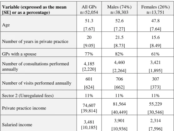
4.4. Practice characteristics
Male and female GPs with a rather low part of the medical activity as employee received lower private practice incomes than those only practicing in private practice. While this average effect was significantly negative for all GPs resulting to the time constraint, this effect appeared to be greater for female GPs (-8%) than for male GPs (-3%). In this case, QR did not provide additional results. GPs with a rather large part of their medical activity as employee also received lower private practice incomes than those only working in private practice. Moreover, QR allowed showing that the income gap between GPs who conducted a large portion of their medical activity as employee and those only practicing in private practice was much larger for female than for male GPs along the incomes distribution. At the lower end of the distribution, the gap reached –58% for female GPs and -43% for male GPs. These gaps were smaller at the upper end of the distribution. The graphs are shown in Figure 4.
15
Concerning the provision of specialized procedures, the OLS results clearly showed that frequently performing specialized procedures significantly increased the private practice income (by over 20% for male GPs and over 26% for female GPs). Moreover, for male and female GPs, the impact of frequently performing specialized procedures appeared to differ along the distribution (see Figure 4).
And finally, participation in ongoing care had a significantly positive effect on private practice income according to OLS results and this effect was particularly high for women (+17% vs. + 7% for male GPs). Throughout the incomes distribution, the QR estimates emphasized the decreasing effect of participating in ongoing care for male and female GPs (see Figure 4).
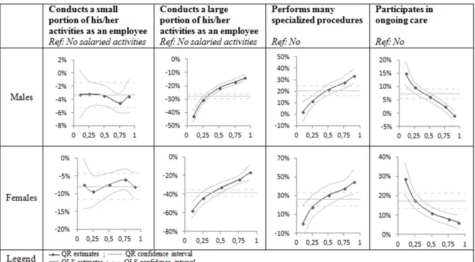
Type of practice
Being a MEP physician led to receive a lower private practice income according to OLS results (-6% for male GPs and -13% for female GPs). QR estimates showed that its impact on private practice income decreased along the incomes distribution for male and female GPs. The graphs are shown in Figure 5.
Similarly, belonging to sector 2 decreased the private practice income by nearly 10% for both male and female GPs. For this covariate, the QR did not provide any additional information (see Figure 5).
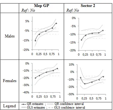
GPs’ casemix
The OLS regression estimates yielded some interesting results for GPs’ casemix. For male and female GPs, having a large number of female patients tended to reduce private practice income by 4-5% on average. On the contrary, for all GPs, having a large proportion of children in the casemix increased the private practice income. This effect was stronger for female GPs (almost 22%) than for male GPs (16%). Finally, having a large proportion of
16
elderly in the casemix appeared to have no impact on private practice income for males but to have a positive impact on private practice income for females (+10%). The QR estimates provided some interesting additional results, particularly for children and elderly patients. Male and female GPs having a high percentage of children in the casemix received a higher private practice income than other GPs across all quantiles. This effect was significantly very high +39% for female and +25% for male GPs but decreased along the incomes distribution to reach +11% for female and +7% for male GPs. Nevertheless, at all quantiles, the effect was higher for female GPs. The graphs are shown in Figure 6.
Even more interestingly, the QR results showed that male GPs having a high proportion of elderly in the casemix had significantly higher private practice income than others GPs (+4%) at the lower end of the males GPs incomes distribution. This effect decreased to become significantly negative from the quantile 0.5 to reach -8% at the highest quantile. Women, having a high proportion of elderly in the casemix had higher private practice income than others female GPs across the incomes distribution, but this effect decreased along the quantiles and became insignificant in the highest quantile (see Figure 6).
Insert Figure 4 Insert Figure 5 Insert Figure 6
4.5. Contextual variables
Practicing in a low-medical-density area compared to a high-medical-density area generated a higher private practice income for male and female GPs. The income gap was much higher for female GPs (+18%) than for male doctors (+14%) and tended to decrease as the density of GPs increased. Conditional on other factors (including the density of GPs), GPs in rural area
17
had higher private practice income. However, the effect appeared to be slightly lower for female GPs (+5%) than for male doctors (+6%). For this covariate, QR did not provide additional information. The graphs are shown in Figure 7.
Insert Figure 7
5. DISCUSSION
From an exhaustive database of GPs working in private practice in France in 2008, we conducted a number of analyses to understand the specific roles played by various factors in generating private practice income for male and female GPs. Moreover, for all covariates, we ran OLS and QR regressions to first evaluate the average effect of each factor conditionally to all others and second, to measure the potential variation in the effects along the incomes distribution for male and female GPs separately.
While for some covariates, QR did not provide additional information compared to the results of OLS regression, for some others, QR brought some interesting original results.
An interesting contribution of our study is to take into account the individual implicit trade-off between leisure and working time within the household by considering the household structure (couples, singles with children) and/or the spouse's income. We also identify the physicians whose spouses are doctors (not necessarily GPs). The results are interesting because they show that the trade-offs realized by doctors differ according to both gender and household structure. For instance, single GPs had lower private practice income than GPs with a spouse earning less than €2,000 monthly: while for male GPs, this difference in incomes (associated to household status) varies along the distribution, it remains rather stable for female GPs across all quantiles. These results are coherent with previous studies (Rizzo and Blumenthal, 1994; Bashaw and Heywood, 2001). When a GP has a spouse, his or her
18
income tends to decrease as the spouse’s income increases. As shown by Sobecks et al. (1999) and Woodward (2005), dual physician couples appear to adopt different behaviors. GPs with a physician spouse had lower income than GPs with a spouse earning less than €2,000. This income gap appeared to be higher than those between GPs with a spouse with high income (more than €2000) and GPs with a spouse earning less than €2,000.
In addition to private practice, GPs may also participate in some salaried activities. The results are as expected: a wage increase is associated with a decrease in private practice income resulting probably of working time substitution. However, for female GPs, the effect of salaried activity is higher than for males, resulting in a greater substitution effect, potentially due to the more restrictive time constraints. Regarding participation in ongoing care, the interpretation is very similar, and again, the effect appears to be stronger for women.
An interesting result of our paper is related to the effect of the GPs’ casemix. The patients’ profiles are known to be an important determinant of medical services but not directly of income in the context of a FFS system. For male and female GPs, having a large number of female patients tends to reduce income on average. This result could be due to the length of consultations with women, which are longer on average (Bensing et al., 1993) particularly when the GP is also a woman (Carr-Hill et al., 1998). Male and female GPs with a high percentage of children in their casemix have a higher private practice income than other GPs along the incomes distribution, but this effect decreases as income rises. Even more interesting, we emphasize adverse effects of the number of elderly in the casemix along the distribution of private practice incomes through QR results: for instance, for males GPs, whereas the OLS estimates testify a non-significant effect, QR results show a significant positive effect at the lower end of the distribution and a significant negative effect at the higher end. Indeed, for a male GP belonging to the 10% of GPs earning the most, it is clear that having a high proportion of patients over 65, reduces the private practice income by -8%
19
(compared to other male GPs in the same quantile). Conversely, male GPs in the first conditional quantile, belonging to the 10% of GPs earning the least benefit from having a high percentage of elderly patients as they receive a higher income (+4%) compared to other male GPs. For female GPs, the effect remains positive, although it decreased significantly as conditional income increases. This result is particularly interesting because the FFS system is not known to favor the selection of certain patients by doctors. Our results do not precisely indicate whether doctors actually select patients or not, but some of them could clearly have an interest in doing so: a male GP at the upper end of the incomes distribution may have no interest or even be discouraged to accept an elderly in the casemix. This finding could be the result of the characteristics of these patients, who often require long consultations (Breuil-Genier and Gofette, 2006). While we can control for the provision of specialized procedures, this result is an illustration of the limit of a FFS system that is supposed to base payment on a ‘standardized’ consultation. While the fee (regulated) is supposed to include all costs on average, it seems that the calculation fails to take sufficiently and correctly into account some of these costs such as the duration of the consultation or the complexity of the disease. On the argument of the necessity to reduce or eradicate induced demand potentially generated by FFS, (Bardey, 2002) justified to introduce a payment per pathology in ambulatory care. Here, on a different argument ‘to avoid potential patient selection’, our study suggests that fees better adjusted to patient profiles may help in avoiding incentives for patient selection. This may become even more essential in a context of a decrease in primary care supply i.e. where doctors would have to provide more care with strong geographical inequalities and thus, despite the fact that FFS is not really known to favor patient selection.
20
6. REFERENCES
Attal-Toubert, K., Fréchou, H., Guillaumat-Tailliet, F., 2009. Le revenu global d’activité des médecins ayant une activité libérale. Insee: Références, Les revenus d’activité des
indépendants.
Auer, P., Gazier, B., 2002. L’articulation entre travail et famille, in: L’avenir Du Travail, De L’emploi Et De La Protection Sociale, Compte Rendu Du Symposium France/OIT.
Organisation internationale du travail.
Bardey, D., 2002. Demande induite et réglementation de médecins altruistes. Revue économique 53, 581–588.
Bashaw, D.J., Heywood, J.S., 2001. The Gender Earnings Gap for US Physicians: Has Equality been Achieved? Labour 15, 371–391.
Béjean, S., Peyron, C., Urbinelli, R., 2007. Variations in activity and practice patterns: a French study for GPs. The European Journal of Health Economics 8, 225–236.
Bensing, J.M., van den Brink-Muinen, A., de Bakker, D.H., 1993. Gender differences in practice style: a Dutch study of general practitioners. Med Care 31, 219–229.
Breuil-Genier, P., Gofette, C., 2006. La durée des séances des médecins généralistes. Etudes et Résultats, French Ministry of Health.
Buchinsky, M., 1998. Recent Advances in Quantile Regression Models: A Practical Guideline for Empirical Research. The Journal of Human Resources 33, 88.
Carr-Hill, R., Jenkins-Clarke, S., Dixon, P., Pringle, M., 1998. Do minutes count? Consultation lengths in general practice. J Health Serv Res Policy 3, 207–213.
Clerc, I., L’haridon, O., Paraponaris, A., Protopopescu, C., Ventelou, B., 2012. Fee-for-service payments and consultation length in general practice: a work–leisure trade-off model for French GPs. Applied Economics 44, 3323–3337.
Dedobbeleer, N., Contandriopoulos, A.P., Desjardins, S., 1995. Convergence or divergence of male and female physicians’ hours of work and income. Med Care 33, 796–805.
Delattre, E., Dormont, B., 2003. Fixed fees and physician-induced demand: a panel data study on French physicians. Health Econ 12, 741–754.
Desprès, P., 2010. Santé physique et psychique des médecins généralistes. Etudes et Résultats, French Ministry of Health.
Dormont, B., Samson, A.-L., 2008. Medical demography and intergenerational inequalities in general practitioners’ earnings. Health Econ 17, 1037–1055.
Dumontet, M., Le Vaillant, M., Franc, C., 2012. What determines the income gap between French male and female GPs - the role of medical practices. BMC Fam Pract 13, 94.
Dusmesnil, H., Serre, B.S., Régi, J.-C., Leopold, Y., Verger, P., 2009. Professional burn-out of general practitioners in urban areas: prevalence and determinants. Sante Publique 21, 355– 364.
21
Fauvet, L., Romain, O., Buisine, S., Laurent, P., 2012. Les affectations des étudiants en médecine à l’issue des épreuves classantes nationales en 2011. Etudes et Résultats, French Ministry of Health.
Franc, C., Lesur, R., 2004. Systèmes de rémunération des médecins et incitations à la prévention. Revue économique 55, 901.
Fujisawa, R., Lafortune, G., 2008. The remuneration of general practitioners and specialists in 14 OECD countries: what are the factors influencing variations across countries? Editions de l’OCDE, Documents de travail de l’OCDE sur la santé.
Koenker, R., Bassett, G., 1978. Regression Quantiles. Econometrica 46, 33.
Koenker, R., Hallock, K.F., 2001. Quantile Regression. Journal of Economic Perspectives 15, 143–156.
Kroneman, M.W., Van der Zee, J., Groot, W., 2009. Income development of General Practitioners in eight European countries from 1975 to 2005. BMC Health Serv Res 9, 26. Mincer, J.A., 1974. The Human Capital Earnings Function (NBER Chapters). National Bureau of Economic Research, Inc.
Rizzo, J.A., Blumenthal, D., 1994. Physician labor supply: Do income effects matter? Journal of Health Economics 13, 433–453.
Rochaix, L., 2004. Les modes de rémunération des médecins. Revue d'économie financière 76, 223–239.
Samson, A.-L., 2006. La dispersion des honoraires des omnipraticiens sur la période 1983-2004 : une application de la méthode des régressions quantiles. Série Etudes, French Ministry of Health.
Samson, A.-L., 2011. Do French low-income GPs choose to work less? Health Econ 20, 1110–1125.
Sasser, A.C., 2005. Gender Differences in Physician Pay: Tradeoffs between Career and Family. The journal of human Resources 40, 447–504.
Shih, Y.-C.T., Konrad, T.R., 2007. Factors associated with the income distribution of full-time physicians: a quantile regression approach. Health services research 42, 1895–1925. Sobecks, N.W., Justice, A.C., Hinze, S., Chirayath, H.T., Lasek, R.J., Chren, M.M., Aucott, J., Juknialis, B., Fortinsky, R., Youngner, S., Landefeld, C.S., 1999. When doctors marry doctors: a survey exploring the professional and family lives of young physicians. Ann. Intern. Med. 130, 312–319.
Theurl, E., Winner, H., 2011. The male–female gap in physician earnings: evidence from a public health insurance system. Health Econ 20, 1184–1200.
Véga, A., Cabé, M.-H., Blandin, O., 2008. Cessation d’activité libérale des médecins généralistes : motivations et stratégies. Dossiers solidarité et santé, French Ministry of Health.
22
Woodward, C.A., 2005. When a physician marries a physician: effect of physician-physician marriages on professional activities. Can Fam Physician 51, 850–851.
23
Appendix A: Variable definitions
Variable Definition
1) Personal characteristics
Number of years in private practice
Number of years in private practice, squared
Single =1 if the GP is single
Has a non-physician spouse with no income =1 if the GP has a non-physician spouse with no income Has a non-physician spouse with an
income≥€2,000per month
=1 if the GP has a non-physician spouse who earns more than €2,000per month
Has a physician spouse =1 if the GP has a physician spouse
Has children =1 if the GP has children
2) Practice characteristics
Conducts a small portion of his/her activities as an
employee =1 if the GP receives a salary >€0 and <€10,000 per year
Conducts a large portion of his/her activities as an
employee =1 if the GP receives a salary ≥€10,000 per year
Performs many specialized procedures =1 if specialized procedures represent more than 10% of his/her private practice activity
Participates in ongoing care =1 if the GP participates in ongoing care
MEP physician =1 if the GP is an MEP physician
Sector2 =1 if the GP receives unregulated fees
Has many women in his/her casemix =1 if the proportion of women in his/her casemix is greater than
or equal to the mean (0.56)
Has many children in his/her casemix =1 if the proportion of children under 16 years old in his/her casemix is greater than or equal to the mean (0.19)
Has many elderly in his/her casemix =1 if the proportion of elderly (over 65 years old) in his/her casemix is greater than the mean (0.17)
3) Location characteristics
Area with a low GP/population ratio =1 if the GP works in an area with a GP/population ratio less than or equal to 90 per 100,000 inhabitants
Area with a moderate GP/population ratio =1 if the GP works in an area with a GP/population ratio greater than 90 and less than or equal to 115 per 100,000 inhabitants
24
Appendix B: Results table Parameter Estimates for Male GPs
Parameter OLS 0.1 0.25 0.5 0.75 0.9
Intercept 10.8 *** 10.1 *** 10.6 *** 10.9 *** 11.3 *** 11.5 ***
Number of years in private
practice 1.8% *** 2.1% *** 2.0% *** 1.7% *** 1.6% *** 1.4% ***
Number of years in private
practice, squared -0.041% *** -0.05% *** -0.05% *** -0.04% *** -0.03% *** -0.03% ***
Single GP -17% *** -26% *** -19% *** -14% *** -11% *** -9% ***
Has a non-physician
spouse with no income 13% *** 17% *** 14% *** 11% *** 10% *** 10% ***
Has a non-physician spouse with an income
≥€2,000 per month -10% *** -13% *** -11% *** -8% *** -8% *** -7% ***
Has a physician spouse -12% *** -16% *** -14% *** -11% *** -9% *** -7% ***
Has children 12% *** 18% *** 11% *** 9% *** 6% *** 6% ***
Conducts a small portion of his activities as an employee
-3% *** -3% ** -3% *** -3% *** -5% *** -3% ***
Conducts a large portion of his activities as an employee
-28% *** -43% *** -31% *** -22% *** -17% *** -14% ***
Performs many specialized
procedures 20% *** 2% NS 11% *** 21% *** 27% *** 33% ***
Participates in ongoing
care 7% *** 15% *** 10% *** 6% *** 2% *** -1% NS
MEP physician -6% *** -15% *** -9% *** -5% *** -2% * 3% *
Sector 2 -10% *** -13% *** -11% *** -9% *** -9% *** -8% ***
Has many women in his
casemix -4% *** -6% *** -4% *** -1% NS -1% NS -1% NS
Has many children in his
casemix 16% *** 25% *** 16% *** 12% *** 9% *** 7% ***
Has many elderly in his
casemix 0% NS 4% *** 1% NS -2% *** -4% *** -8% ***
Area with a low
GP/population ratio 14% *** 20% *** 15% *** 12% *** 9% *** 9% ***
Area with a moderate
GP/population ratio 9% *** 15% *** 10% *** 8% *** 6% *** 7% ***
Rural area 6% *** 6% *** 6% *** 6% *** 6% *** 6% ***
25
Parameter Estimates for Female GPs
Parameter OLS 0.1 0.25 0.5 0.75 0.9
Intercept 10.32 *** 9.34 *** 10.01 *** 10.51 *** 10.88 *** 11.16 ***
Number of years in private
practice 3% *** 4% *** 3% *** 3% *** 2% *** 2% ***
Number of years in private
practice, squared -0.07% *** -0.10% *** -0.08% *** -0.06% *** -0.05% *** -0.05% ***
Single GP -7% *** -3% NS -7% *** -9% *** -9% *** -8% ***
Has a non-physician
spouse with no income 15% *** 14% *** 11% *** 13% *** 14% *** 16% ***
Has a non-physician spouse with an income
≥€2,000 per month -11% *** -11% *** -11% *** -10% *** -10% *** -11% ***
Has a physician spouse -20% *** -30% *** -20% *** -16% *** -15% *** -13% ***
Has children 12% *** 21% *** 13% *** 7% *** 4% *** 3% **
Conducts a small portion of her activities as an employee
-8% *** -7% *** -9% *** -7% *** -6% *** -8% ***
Conducts a large portion of her activities as an employee
-39% *** -58% *** -45% *** -33% *** -24% *** -17% ***
Performs many specialized
procedures 26% *** 0% NS 17% *** 30% *** 37% *** 44% ***
Participates in ongoing
care 17% *** 29% *** 18% *** 11% *** 8% *** 6% ***
MEP physician -13% *** -20% *** -17% *** -12% *** -10% *** -7% ***
Sector 2 -10% *** -7% NS -16% *** -13% *** -10% *** -6% *
Has many women in her
casemix -5% *** -1% NS -3% NS -5% *** -8% *** -8% ***
Has many children in her
casemix 22% *** 39% *** 25% *** 17% *** 14% *** 11% ***
Has many elderly in her
casemix 10% *** 16% *** 10% *** 7% *** 4% *** 0% NS
Area with a low
GP/population ratio 18% *** 30% *** 21% *** 16% *** 14% *** 14% ***
Area with a moderate
GP/population ratio 30% *** 18% *** 12% *** 11% *** 10% *** 10% ***
Rural area 5% *** 5% ** 8% *** 6% *** 6% *** 5% ***
26 TABLES
Table 1: Description of the GP population
Variable (expressed as the mean [SE] or as a percentage) All GPs n=52,054 Males (74%) n=38,303 Females (26%) n=13,751 Age 51.3 [7.67] 52.6 [7.27] 47.8 [7.64] Number of years in private practice 20
[9.05] 21.5 [8.73] 15.6 [8.49] GPs with a spouse 77% 82% 61%
Number of consultations performed annually 4,185 [2,220] 4,460 [2,264] 3,421 [1,895] Number of visits performed annually 601
[624]
706 [662]
307 [373]
Sector 2 (Unregulated fees) 11% 11% 11%
Private practice income 74,607
[39,814] 81,564 [40,449] 55,229 [30,546] Salaried income 3,481 [10,185] 3,901 [10,936] 2,314 [7,596]
27
Table 3: Descriptive Statistics
Variable (expressed as the mean [SE] or as a percentage)
All GPs Male GPs Female GPs
Mean Mean Mean
Personal characteristics
Length of experience
Number of years in private practice 20 [9.05] 21.5 [8.73] 15.6 [8.49] Household composition
Single GP 23% 18% 39%
Has a non-physician spouse with no income 20% 27% 3%
Has a non-physician spouse with an income
<€2,000 per month 24% 27% 10%
Has a non-physician spouse with an income
≥€2,000 per month 22% 20% 29%
Has a physician spouse 11% 8% 19%
Has children 63% 61% 67%
Practice characteristics
Physician activities
Conducts a small portion of his/her activities as an
employee 17% 18% 16%
Conducts a large portion of his/her activities as an
employee 11% 12% 7%
Performs many specialized procedures 7% 6% 10%
Participates in ongoing care 51% 53% 44%
Type of practice
Mep GP 11% 9% 16%
Sector 2 11% 11% 11%
GPs’ casemix
Has many women in his/her casemix 43% 28% 87%
Has many children in his/her casemix 58% 56% 64%
Has many elderly in his/her casemix 43% 48% 31%
Context variables
Area with a low GP/population ratio 23% 23% 23%
Area with a moderate GP/population ratio 52% 53% 50%
Rural area 17% 19% 14%
28
FIGURES
29
30
31
32
33
34
35