Thermochemical-based poroelastic modelling of salt crystallization, and a new multiphase flow experiment : how to assess injectivity evolution in the context of CO2 storage in deep aquifers

HAL Id: tel-00958697

https://pastel.archives-ouvertes.fr/tel-00958697v2

HAL is a multi-disciplinary open access archive for the deposit and dissemination of sci-entific research documents, whether they are pub-lished or not. The documents may come from teaching and research institutions in France or abroad, or from public or private research centers.

L’archive ouverte pluridisciplinaire HAL, est destinée au dépôt et à la diffusion de documents scientifiques de niveau recherche, publiés ou non, émanant des établissements d’enseignement et de recherche français ou étrangers, des laboratoires publics ou privés.

crystallization, and a new multiphase flow experiment :

how to assess injectivity evolution in the context of CO2

storage in deep aquifers

Florian Osselin

To cite this version:

Florian Osselin. Thermochemical-based poroelastic modelling of salt crystallization, and a new mul-tiphase flow experiment : how to assess injectivity evolution in the context of CO2 storage in deep aquifers. Other. Université Paris-Est, 2013. English. �NNT : 2013PEST1136�. �tel-00958697v2�

Thèse présentée pour obtenir le grade de

Docteur de l’Université Paris-Est

Spécialité : Sciences de l’ingénieur

par

Florian Osselin

Ecole Doctorale : Sciences, Ingénierie et Environnement

Thermochemical-based poroelastic modelling of salt crystallization, and a new multiphase flow experiment : how to assess injectivity

evolution in the context of CO₂ storage in deep aquifers ?

Modélisation thermochimique et poroélastique de la cristallisation de sel, et nouveau dispositif expérimental d’écoulement multiphasique : comment prédire l’évolution de l’injectivité pour le stockage du CO₂ en

aquifère profond ?

Thèse soutenue le 20 décembre 2013 devant le jury composé de : Gilles Pijaudier-Cabot Université de Pau Président

et des Pays de l’Adour

Jan Carmeliet ETH Zürich Rapporteur

Lionel Mercury Université d’Orléans Rapporteur François Renard Université Joseph Fourier Examinateur

Arnault Lassin BRGM Examinateur

Antonin Fabbri ENTPE Conseiller d’études

Jean-Michel Pereira ENPC Conseiller d’études

Patrick Dangla IFSTTAR Invité

Remerciements

Une thèse n’est jamais le travail d’une seule personne et celle-ci ne fait pas exception. J’ai eu la chance durant ces travaux d’être encadré par une équipe efficace et toujours présente pour répondre à mes questions et qui m’a énormément apporté tant sur le plan scientifique qu’humain. Je voudrais ainsi remercier Teddy Fen-Chong mon maître de thèse pour sa patience, ses bons conseils et son efficacité, Patrick Dangla pour toutes ces discussions acharnées, Jean-Michel Pereira pour son calme et pour m’avoir tenu compagnie durant toutes ces conférences et réunions, Antonin Fabbri pour sa bonne humeur et Arnault Lassin qui a repris le projet SALTCO au pied levé tout en répondant toujours présent pour les questions de géochimie. Je tiens aussi à remercier Laurent André qui a lui aussi toujours pris le temps de répondre à mes nombreuses interrogations sur le transport réactif.

Ces travaux été possibles grâce aux financement de l’ADEME à travers le projet SALTCO (no. 1094C0013), et de la chaire CTSC (Captage Transport et Stockage du CO₂) que je remercie sincèrement.

Je souhaite également remercier les deux rapporteurs de cette thèse Jan Carmeliet et Lionel Mercury ainsi que les autres membres du jury, Gilles-Pijaudier-Cabot et François Renard pour m’avoir fait l’honneur de lire ce manuscrit et d’avoir participé à ma soutenance.

Cette thèse a aussi été l’histoire d’une longue lutte avec ce prototype de percolation réactive. Je tiens à remercier David Hautemayou pour son soutien technique et Cédric Mezière pour m’avoir laissé lui emprunter tous ses outils.

J’ai eu aussi la chance de travailler dans un environnement particulièrement chaleureux, et pour cela je tiens à remercier toutes les personnes de Képler, en particulier les thésards : mes co-bureaux Adrien, Mathilde et Antoine, et tous les autres : Benjamin, Benoît, Claire, Guillaume, Lucie, Manu, Marine, Michel, Thibaud. Merci pour tous ces bons moments passés en votre compagnie.

Enfin un grand merci à ma famille et à mes amis pour m’avoir supporté durant ces trois ans. Merci en particulier à Alexia qui a toujours cru en moi et m’a toujours poussé à donner le meilleur de moi-même.

Résumé

Dans un contexte de réduction internationale des émissions de gaz à effet de serre, les techniques de Captage Transport et Stockage de CO₂ (CTSC) apparaissent comme une solution à moyen terme particulièrement efficace. En effet, les capacités de stockage géo-logique pourraient s’élever jusqu’à plusieurs millions de tonnes de CO₂ injectées par an, soit une réduction substantielle des émissions atmosphériques de ce gaz. Une des cibles privilégiées pour la mise en place de cette solution sont les aquifères salins profonds. Ces aquifères sont des formations géologiques contenant une saumure dont la salinité est sou-vent supérieure à celle de la mer la rendant impropre à la consommation. Cependant, cette technique fait face à de nombreux défis technologiques ; en particulier la précipitation des sels, dissous dans l’eau présente initialement dans l’aquifère cible, suite à son évaporation par le CO₂ injecté. Les conséquences de cette précipitation sont multiples, mais la plus importante est une modification de l’injectivité, c’est-à-dire des capacités d’injection. La connaissance de l’influence de la précipitation sur l’injectivité est particulièrement im-portante tant au niveau de l’efficacité du stockage et de l’injection qu’au niveau de la sécurité et de la durabilité du stockage. Le but de ces travaux de thèse est de comparer l’importance relative des phénomènes négatif (colmatage) et positif (fracturation) consé-cutifs à l’injection de CO₂ et à la précipitation des sels. Au vu des nombreux résultats de simulations et de modélisation dans la littérature décrivant le colmatage de la porosité, il a été décidé de porter l’accent sur les effets mécaniques de la cristallisation des sels et la possible déformation de la roche mère. Une modélisation macroscopique et microscopique, tenant compte de deux modes possibles d’évaporation induits par la distribution spatiale de l’eau résiduelle a donc été développée afin de prédire le comportement mécanique d’un matériau poreux soumis à un assèchement par injection de CO₂. Les résultats montrent que la pression de cristallisation consécutive à la croissance d’un cristal en milieu confiné peut atteindre des valeurs susceptibles localement de dépasser la résistance mécanique du matériau, soulignant ainsi l’importance de ces phénomènes dans le comportement méca-nique global de l’aquifère. Sur le plan expérimental, les travaux ont porté sur l’utilisation d’un nouveau prototype de percolation réactive afin de reproduire le comportement d’une carotte de roche soumise à l’injection et ainsi obtenir l’évolution des perméabilités dans des conditions similaires à celle d’un aquifère.

Abstract

In a context of international reduction of greenhouse gases emissions, CCS (CO₂ Capture and Storage) appears as a particularly interesting midterm solution. Indeed, geological storage capacities may raise to several millions of tons of CO₂ injected per year, allowing to reduce substantially the atmospheric emissions of this gas. One of the most interesting targets for the development of this solution are the deep saline aquifers. These aquifers are geological formations containing brine whose salinity is often higher than sea water’s, making it unsuitable for human consumption. However, this solution has to cope with numerous technical issues, and in particular, the precipitation of salt initially dissolved in the aquifer brine. Consequences of this precipitation are multiple, but the most important is the modification of the injectivity i.e. the injection capacity. Knowledge of the influence of the precipitation on the injectivity is particularly important for both the storage effi-ciency and the storage security and durability. The aim of this PhD work is to compare the relative importance of negative (clogging) and positive (fracturing) phenomena following CO₂ injection and salt precipitation. Because of the numerous simulations and modelling results in the literature describing the clogging of the porosity, it has been decided to focus on the mechanical effects of the salt crystallization and the possible deformation of the host rock. A macroscopic and microscopic modelling has then been developed, taking into account two possible modes of evaporation induced by the spatial distribution of residual water, in order to predict the behavior of a porous material subjected to the drying by carbon dioxide injection. Results show that crystallization pressure created by the growth of a crystal in a confined medium can reach values susceptible to locally exceed the mechanic resistance of the host rock, highlighting the importance of these phenomena in the global mechanical behavior of the aquifer. At the experimental level, the study of a rock core submitted to the injection of supercritical carbon dioxide has been proceeded on a new reactive percolation prototype in order to obtain the evolution of permeabilities in conditions similar to these of a deep saline aquifer.

Contents

List of Tables xxi

List of symbols xxiii

General introduction 1

I

Injection of supercritical carbon dioxide in deep saline

aquifers

3

1 Context of the study 5

1.1 Carbon dioxide and greenhouse effect . . . 6

1.2 Political decisions and solutions . . . 8

1.2.1 International conferences and political decisions . . . 8

II

Thermo-Hydro-Chemical behavior of the aquifer

13

3 Hydrodynamic behavior of the aquifer 15

3.1 Porosities and phase saturations . . . 16

3.1.1 Definitions . . . 16

3.1.2 Diagenesis and the formation of natural porous media . . . 17

3.2 Mass balance and fluid velocity . . . 18

3.2.1 Mass Balance . . . 18

3.2.2 Fluid velocity: Darcy’s law and relative permeabilities . . . 19

3.2.3 Displacement of dissolved species: diffusion . . . 20

3.2.4 Klinkenberg effect . . . 20

3.3 Surface energy and consequences . . . 21

3.3.1 Interfacial energy and wettability . . . 21

3.3.2 Capillary pressure . . . 23

3.4 Hydrodynamic regimes . . . 25

4 Chemical behavior of the aquifer 29 4.1 Carbon dioxide/brine partitioning . . . 30

4.1.1 Thermodynamics of mixtures . . . 30

4.1.2 Molar quantities of reaction . . . 34

4.1.3 Laws for CO2/H2O partitioning . . . 36

4.1.4 Activity and fugacity coefficients . . . 38

4.1.5 Kinetics of evaporation and simplifications . . . 40

4.2 Chemical reactions induced by carbon dioxide dissolution (mineral trapping) 41 4.2.1 Carbon dioxide dissolution and pH evolution . . . 41

4.2.2 Mineral reactions and carbon dioxide trapping . . . 42

4.2.3 Kinetics of mineral reactions: nucleation and crystal growth . . . . 44

4.2.4 Porosity and permeability variations induced from dissolu-tion/precipitation . . . 50

5 Thermal behavior of the aquifer 53 5.1 Joule-Thomson expansion . . . 54

5.2 Heat of reaction . . . 54

5.3 Thermal diffusion . . . 55

5.4 Importance of the different phenomena . . . 56

6 Summary of the THC behavior of the aquifer 57 6.1 TOUGH, an intensively used family of codes . . . 58

6.2 Presentation of different simulations . . . 59

6.3 Summary of the simulations: the THC Behavior . . . 59

III

Modellings and simulations

63

7.1.1 Presentation and definitions . . . 66

7.1.2 Frame of the Study and Constitutive Hypothesis . . . 66

7.2 Constitutive equations of unsaturated poroelasticity . . . 67

7.3 Application of the equations to the CCS case . . . 69

8 Thermodynamics of in-pore crystallization 73 8.1 Ostwald-Freundlich equation and Wulff theorem . . . 74

8.1.1 Chemical equilibrium of a crystal in solution . . . 74

8.1.4 Non-flat surfaces . . . 77

8.2 Interaction energy between two solid surfaces . . . 78

8.2.1 Equilibrium of a crystal surface close to the pore wall . . . 78

8.2.2 Expression of the interaction energy . . . 82

8.3 In-pore growth of a single crystal and crystallization pressure . . . 84

8.3.1 First case: crystallization pressure in a cylindrical pore . . . 84

8.3.2 Second case: crystallization pressure in a spherical pore with small entry channels . . . 85

8.3.3 Crystallization pressure and Wulff shape . . . 88

8.3.4 Thickness δ and interaction forces . . . . 91

8.3.5 Effectively transmitted stress . . . 92

8.4 Final remark . . . 93

9 Estimation of crystallization pressure in the case of CCS 95 9.1 Macroscopic behavior: poromechanics at the REV scale . . . 96

9.1.1 Modelling at constant concentration . . . 96

9.1.2 Simulation of a REV submitted to carbon dioxide evaporation . . . 106

9.1.3 Comparison of the two modellings . . . 115

9.2 Microscopic behavior: nucleation and stress creation at the pore level . . . 117

9.2.1 Evolution of the salt quantity in the corner . . . 117

9.2.2 Algorithm . . . 122

9.2.3 Results of the simulation . . . 125

9.2.4 Nucleation and crystal growth . . . 127

9.2.5 Upscaling and poromechanics . . . 130

IV

Experimentation of reactive percolation

137

10 General purpose of the experiments 139

11 Description of the set-up and characteristics 141

11.1 Description and sketch of the prototype . . . 142

11.1.1 Material . . . 142

11.1.2 Description of the different parts of the set-up . . . 145

11.2 Dead volumes measurement . . . 152

11.2.1 Method . . . 153

11.2.2 Results . . . 153

12 Rock cores and sintered glass 157 12.1 Rock cores . . . 158

12.1.1 Pierre de Lens . . . 158

12.1.2 Grès des Vosges . . . 158

12.1.3 Rocks from the Dogger aquifer of the Paris Basin . . . 158

12.2 Sintered glass beads . . . 160

12.2.1 Sintering temperature and duration . . . 160

12.2.2 Moulding of the material . . . 160

12.2.3 Shrinkage and density profile . . . 163

12.3 Mercury Intrusion Porosimetry of the different cores . . . 164

12.3.1 Principle of the measurement . . . 164

12.3.2 Material and methods . . . 164

12.3.3 Results . . . 165

13 Intrinsic and relative permeability measurement 167 13.1 Intrinsic permeability . . . 168

13.2 Relative permeability . . . 171

13.2.1 Methods . . . 171

13.2.2 Results . . . 175

13.3 Capillary pressure measurement . . . 178

13.3.1 Method . . . 178

13.3.2 Results . . . 178

13.4 Issues and solutions . . . 180

13.4.1 Carbon dioxide pressure and leakage . . . 180

13.4.2 BPV oscillations . . . 181

13.4.3 Meniscus and sensor in the separator . . . 182

13.4.4 Precipitation in the gasometer . . . 183

14 Drying-out measurement 185 14.1 Purpose . . . 186

14.2 Issues and solutions . . . 186

14.3 Addendum . . . 187

General conclusion 191 Bibliography 204

Appendices

207

A.2 Fugacities . . . 211

C Correlation of the equilibrium constant 221

D Capillary pressure curve estimation from mercury intrusion porosimetry225

E Correlation between maximum pore radius and water saturation 229

F Analysis of the Grès des Vosges (BRGM) 233

List of Figures

1.1 Evolution of the anthropic emissions of carbon dioxide since 1800 (from [13]) 6

1.2 Schematic of the greenhouse effect (from [16]) . . . 7

1.3 Evolution of the surface temperature (from NASA-GISS) (in black is the annual mean, in red the 5-year running mean, in green are the uncertainty estimates) . . . 7

1.4 Schematics of the different targets for CCS (from Kaltediffusion.ch) . . . . 9

1.5 Relative efficiency of the different solutions . . . 9

3.1 Illustration of the Lagrangian porosity and the deformation of the porous volume in a two-fluid case (from [20]). . . 17

3.2 Definition of the surface energy as the creation of new surfaces. . . 21

3.3 Sketch of the different wetting situations. . . 22

3.4 Curvature between two fluids in a pore. . . 23

3.5 Evolution of capillary pressure with water saturation Sw in drainage and imbibition conditions (from [40]). . . 24

3.6 Determination of fluid behavior according to the comparison between capil-lary numbers and viscosity ratio. The grey zone represents the zones where the fluids have an undetermined (intermediate) behavior (from [35]. . . 26

3.7 Sketch of the percolation of CO₂ in a porous medium and the different kinds of residual water. The solid matrix is shown in black, water is blue and CO₂ is orange. . . 28

4.1 Sillén diagram for carbon dioxide aqueous species. . . 42

4.4 Modelisation of a conceptual pore (a) with the tubes-in-series model (b), from [80]. . . 51

6.1 Schematic of the aquifer during carbon dioxide injection (from [96]). . . 60

6.2 Distribution of the CO₂ saturation according to numerical simulation (from [97]). . . 61

8.1 Illustration of the Wulff shape for a cubic halite crystal. . . 77

8.2 Vicinal surface of a crystal with an angle θ. . . . 77

8.3 Overlap between the energy profile of two flat surfaces and the creation of the disjoining pressure, adapted from [19]. . . 79

8.4 Crystal growing in a cylindrical pore and the different curvatures (adapted from [107]). . . 84

8.5 Crystal growing in a spherical pore of radius rp and invading the small entry channels of radius rs. The curvature of the crystal in the channel depends on the current supersaturation (adapted from [107]). . . 86

8.6 Particular case of a crystal growing in a cylindrical pore, with tips radius of curvature corresponding to the pore radius (adapted from [107]). . . 88

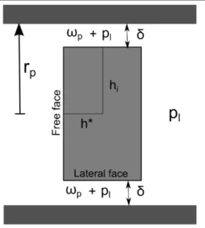
8.7 Halite crystal at homogeneous pressure ps confined in a pore with a square section. . . 89

8.8 Tilted halite crystal at homogeneous pressure confined in a pore with a square section. . . 90

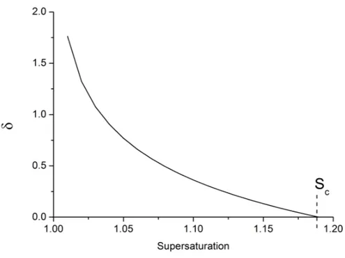
8.9 Evolution of the equilibrium thickness δ with the supersaturation for halite at 40 ℃. . . 92

9.1 Modelling of the porous medium as a succession of spherical pores of de-creasing size linked by cylindrical channels of dede-creasing radius. . . 97

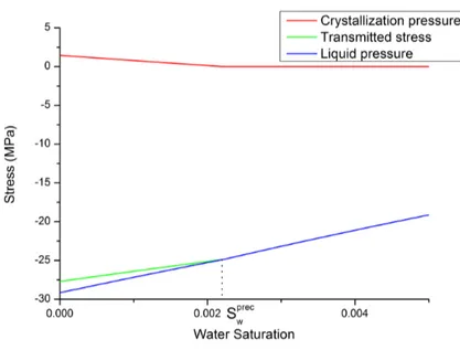
9.2 Decomposition of the transmitted stress into crystallization pressure and liquid pressure for halite at 40 ℃ for the MDV capillary curve. . . 102

9.3 Evolution of the transmitted stress with water saturation for different temperature for hydrohalite/halite 9.3(a) and9.3(c) and the couple anhy-drite/gypsum 9.3(b) and 9.3(d)for the BBL and MDV rocks. . . 103

9.4 Evolution of the equivalent tensile stress with water saturation in a pure water condition. . . 106

9.5 Evolution of the difference in equivalent tensile stress with water satura-tion for different temperature for halite/hydrohalite 9.5(a) and 9.5(c) and gypsum/anhydrite 9.5(b) and 9.5(d)for BBL and MDV rocks. . . 107

9.6 Profiles of liquid pressure 9.6(a), equivalent tensile stress 9.6(b), liquid

9.6(c) and crystal 9.6(d) saturations for BBL at 5mm/s at 196s, MDV at 5mm/s at 12s and MDV at 5µm/s at 14996s. . . . 112

9.7 Comparison of the three equivalent tensile stress obtained with the two macroscopic calculations. . . 116

9.8 Presentation of the capillary trapped water in the corner subjected to evap-oration by CO₂ flowing through the big pore. . . 118

9.9 Speed of growth for a small crystal as a fonction of the radius for constant supersaturation. . . 120

9.10 Description of the evolution of the corner during evaporation and precipi-tation. . . 122

9.11 Algorithm used for the simulation of the behavior of the corner. . . 123

9.12 Pore model used for the calculation. . . 123

9.13 Creation of the crystallization pressure for a spherical crystal close to the pore wall. . . 124

9.14 Evolution of the water saturation and the supersaturation in the pore. . . . 126

9.15 Crystallization pressure corresponding to the supersaturation of figure9.14. 127

9.16 Influence of the CO₂ flow rate (top) and the pore size (bottom) on the maximum crystallization pressure. . . 128

9.17 Evolution of the nucleation rate and the critical radius of nucleation with time. . . 129

9.18 Variation of size for the nuclei at the moment of their creation. . . 129

9.21 Evolution of the distribution of occupied volume with crystal radius. . . 132

9.22 Evolution of the number of nuclei with the flow rate. . . 133

9.23 Upscaling to an REV of the corner. . . 133

9.24 Results of the upscaling: equivalent macroscopic stress and strain. . . 134

11.1 Picture of the experimental set-up. . . 143

11.2 Control panel of the software. . . 144

11.3 Picture of the bottom of the brine reservoir. Picture on the left is a zoom of the center. Note the corrosion on the hole in the center hole. . . 145

11.4 Reaction of sleeves with carbon dioxide. 11.4(a)is the initial sleeve. 11.4(b) and 11.4(c)show sleeves (Viton) after carbon dioxide injection. . . 146

11.5 Cross-section of the triaxial cell. . . 146

11.6 Cross-section of the fluid bottle. . . 147

11.7 Set-up for external experimentation. Note the additional tubing. . . 148

11.8 STIGMA1000 pump (here ST1 and ST3). . . 149

11.9 Sketch of the Back Pressure Valve. . . 150

11.10Phase separator. . . 151

11.11Representation of the considered dead volumes. . . 152

11.12Steel tube for dead volume measurement. . . 153

11.13Determination of dead volume. 11.13(a) represents the dead volume be-tween ST2 and the valve V3 , and 11.13(b) represents the dead volume between the ST2 pump and the BPV. . . 154

12.1 Rock core of Pierre de Lens 12.1(a)and Grès des Vosges 12.1(b) . . . 159

12.2 Temperature program for sintering. . . 161

12.3 Plaster mould used for glass sintering. . . 161

12.5 Result of the glass sintering with quartz tubes: 12.5(a)represents the final cores after trimming, and 12.5(b)represents the cores in their tubes. . . 163

12.6 Schematics of the mercury intrusion porosimetry (MIP). . . 164

12.7 MIP results for the different rock core from the core library. BB =

Bois-Brûlé, MDV = Mondeville, CF1= Clos-Fontaine . . . . 165

12.8 MIP results for Pierre de Lens and Grès des Vosges. . . . 166

12.9 MIP results for two samples of sintered glass. . . 166

13.1 Fit of the evolution of pressure difference after a step increase of injection flow rate. . . 169

13.2 Evolution of the pressure difference with the injection flow rate for a rock core of Pierre de Lens for pure water 13.2(a)and nitrogen 13.2(b). . . 170

13.3 Relative permeability of Pierre de Lens to nitrogen and pure water. . . . . 175

13.4 Relative permeability of Grès des Vosges to supercritical 13.4(a) and gaseous 13.4(b) carbon dioxide and pure water (60 ℃ and 100 bar for supercritical carbon dioxide, 2 bar 20 ℃ for gaseous carbon dioxide). . . . 177

13.5 Capillary pressure curve for the Grès des Vosges sandstone. . . . 180

13.6 Polymer foam to improve the meniscus detection . . . 182

13.7 Precipitation of calcite on the wheel of the gasometer because of the ions in the filling water. . . 183

14.1 Modification of the T junction for salt precipitation. . . 187

14.2 Evolution of the pressure difference during the evaporation with brine sat-uration. The red line is the Savitzki-Golay smoothing on 20 000 points of window . . . 189

B.1 Illustration of a part of the Wulff construction; the red faces make up the final shape of the crystal. . . 215

B.2 Displacement of the surface of a distance dhi (from [136]). . . 216 C.1 Fit of the decimal logarithm of the equilibrium constant with liquid pressure

and the corresponding 4th/6th order polynomial fit. . . 226

E.1 Smoothed derivative of the pore volume as a function of pore radius. . . . 229

E.2 Radius of the biggest pore filled with water for a given water saturation and the corresponding 6th order polynomial fit. . . 230

List of Tables

4.1 Values of the mean electrostatic radius for different solute species. . . 40

4.2 Shape factor for different regular geometries. . . 47

9.1 Relative chemical composition of the brine from the Dogger aquifer in the region of Fontainebleau (in g/kg) from [69]. . . 101

9.3 Input data for the simulations . . . 113

10.1 Historic of the development of the experimental set-up. . . 139

11.1 Color code for the control panel of the system. . . 143

11.2 Technical specifications of the triaxial cell. . . 146

11.3 Technical specifications of the fluid bottle. . . 147

11.4 Technical specifications of the STIGMA 1000 pump. . . 149

11.5 Technical specifications of the back pressure valve (and the micropump). . 150

11.6 Dead volumes in the system. . . 155

13.1 Results of intrinsic permeability. . . 169

13.2 Flow rates used in the measurement of relative permeability of Pierre de

Lens and the corresponding water saturation. The gas used here is nitrogen.172

13.3 Flow rates used in the measurement of relative permeability of Grès des

Vosgesand the corresponding water saturation. The gas used here is carbon dioxide . . . 172

water saturation. . . 173

13.5 Corrected water saturation. . . 174

13.6 Values of capillary pressure and corresponding liquid saturation for the

Grès des Vosges. . . 179

C.1 Correlation coefficients for variation of the equilibrium constant with liquid pressure. . . 223

D.1 Correlation coefficients for the capillary pressure curve (pcap in MPa). . . . 227

E.1 Correlation coefficient for the 6th order fit in figure E.2. . . 231

List of symbols

Symbol Unit Description

Universal constants

~g m.s−2 _{gravitational acceleration}

kB mol−1 Boltzmann constant

N_{a mol}−1 _{Avogadro Number}

R J/K/mol perfect gases constant

ε0 _F.m−1 _{permittivity of the vacuum}

F C.mol−1 _{Faraday constant}

e C elementary charge

Basic symbols

m kg - kg/m3 _{mass or mass per unit volume}

ρ kg/m3 _density

t s time

η Pa.s viscosity

p Pa pressure

pcap Pa capillary pressure

D m2_.s−1 _{diffusion coefficient}

σ J/m2 _{surface energy}

σ∗ _J/m2 _{surface stress}

˜

σ J/m2 _{surface stiffness}

σ′ _J/m2 _{surface energy of a tilted face}

V m3 _volume

υ m3_{/mol molar volume}

T ℃ / K temperature L m length = 1 / identity matrix κ m−1 _curvature r m crystal radius Q m3_{/s flow rate}

Porous medium description

m / solid matrix

n / Eulerian porosity

φ / Lagrangian porosity

Ωpores m3 pore volume

dΩ m3 _{REV volume}

τ / tortuosity

rp m pore radius

rs m entry channel radius

λ / shape ratio of the porous medium

Fluid flow

J,K,L / phases in the porous volume

SJ / saturation of phase J

~ωJ kg/s mass displacement vector of phase J

vJ m/s velocity of phase J ˙ m_J→K kg/s sink/source term nw/w / non-wetting/wetting k0 _m2 _{(D) intrinsic permeability} kr

J / relative permeability of phase J

Slr / residual liquid saturation

Sgr / residual gas saturation

S∗ _{/ reduced water saturation (van}

Genuchten)

Sh / reduced water saturation (Corey)

m / van Genuchten coefficient

̟ Pa characteristic pressure for Klinkenberg

Rh kg.s/m4/ hydraulic resistance

Γ / fractional length of pore bodies in the

tube in series model

ω, θ / parameters for the tube in series model

φr / critical porosity in the tube in series

model

Adimensioned numbers

Ca / capillary number

M / viscosity ratio

Γ / relative importance of evaporation and

crystal growth Basic thermodynamics

G J Gibbs free energy

H J enthalpy

S _{J/K entropy}

Gcomp _{J Gibbs free energy of composition}

Gex _{J excess Gibbs free energy}

Scomp _{J/K entropy of composition}

Scomp _{J/K excess entropy}

u J interaction energy between two

molecules Thermochemistry

µ J/mol chemical potential

ai / chemical activity

fi / fugacity

γi / activity coefficient

γ₊₋ / mean activity coefficient

Φi (β) / fugacity coefficient

ni mol molar quantity of species i

xi / molar fraction of species i

∆r / molar quantity of reaction

∆rG0 _{J/mol standard Gibbs free energy of reaction}

QR / ion activity product (reaction quotient)

Ks / equilibrium constant

S (SR, Ω) / saturation ratio (supersaturation)

SI / saturation index

∆µ J/mol degree of metastability

ξ / extent of reaction

Partitioning

KH Pa Henry’s constant

y / molar fraction in the gas phase

Z / Compressibility factor

Aγ, Bγ kg1/2_/mol1/2

-kg1/2_/mol1/2_/m

Debye-Hückel parameters

◦

a A◦ mean effective electrostatic radius

εr _{/ relative permittivity of the medium}

λw / activity coefficient of water

Analytical chemistry

I / ionic strength

z / charge of an ion

pKa / acidity constant

φ / osmotic coefficient

r mol/s reaction rate

k mol/m2_{/s kinetic constant}

θ, η / kinetic coefficients

Ea J/mol activation energy

Mi g/mol molar mass of species i

Nucleation

∆Gc J/mol nucleation cost

I nuclei/m2_{/s nucleation rate}

K0(T ) nuclei/m2/s prefactor for the nucleation rate

∆Gm J/m nucleation cost fluctuations

λ / nucleation shape factor

α m3 _{volume of a formula unit}

Thermal

µJT K/Pa Joule-Thomson coefficient

δQp J infinitesimal heat variation

Cp J/mol calorific molar capacity

q W/s heat flux

λ W/m2_{/s heat diffusion coefficient}

Poromechanics

Ω / REV

ϕ / porosity variation

sk / skeleton

lh m characteristic length of heterogeneities

lΩ m characteristic length of the REV

L m characteristic length length of the

structure containing Ω ξ / displacement field = ε / strain tensor = Σ Pa stress tensor

Ψ / Helmholtz free energy

ψ / volumetric Helmholtz free energy

w J/m3 _{strain work density}

W J elastic energy stored in the REV

U J energy of the interfaces

p∗

J Pa effective stress of phase J

˜

W J Legendre transform of the elastic

en-ergy

ǫ / volumetric dilatation

Σ Pa mean stress

=

µ Pa shear modulus

bJ Pa Biot coefficient for phase J

NJ Pa Biot modulus for phase J

̟ Pa macroscopic equivalent tensile stress

Crystal description

h m Wulff length

h∗ _{m Wulff length of the free face}

e, δ m film thickness and film thickness at

equilibrium

W J interaction energy

S _J/m2 _{spreading parameter}

ωp Pa disjoining (crystallization) pressure

κ−1 _{m Debye length}

λ0 m characteristic length of the hydration

forces

S∗ _{/ equilibrium supersaturation of a small}

crystal

rc m critical radius for crystal growth

Modelisation

tα g/kg mass proportion of the limiting ion

Sprec

w / precipitation saturation

β / stoichiometric correction

Sprec _{/ nucleation threshold}

◦

Scr s−1 supersaturation variation with crystal-lization

◦

Sev s−1 supersaturation variation with evapora-tion

◦

ξ s−1 _{evaporation rate}

c / averaged radius of pores subjected to

qCO₂ m3/s carbon dioxide flow rate for a single

pore

ωmax

p , ωp∞, τ Pa - Pa - s fit coefficients for the crystallization pressure

General introduction

In the context of increasing environmental concern, CCS (Carbon Capture, transport and geological Storage) appears to be an attractive solution to cope with global warming and increasing carbon dioxide content in the atmosphere. The aim of CCS is to capture carbon dioxide at the exit of the emitters and to store it in the subsurface (offshore or onshore) where it will no longer contribute to greenhouse effect [1]. There are several targets for CCS such as depleted oil and gas reservoirs, unmined coal veins or deep saline aquifers. Deep saline aquifers are huge geological formations containing saline water, unfit for human consumption. The idea is then to inject the carbon dioxide within the porosity of the aquifer and to store it for an indefinite amount of time. This solution seems particularly interesting as storage capacities of deep saline aquifers can raise to several millions of tons of carbon dioxide stored per year [2]. According to the estimations of the International Panel on Climate Change (IPCC [3]), in order to keep the atmospheric concentration of carbon dioxide around the values of 2005, the reduction of emission has to be as important as 15 to 25 Gt CO₂/year, making CCS one of the key solution for reducing carbon dioxide emissions. However, numerous studies on CCS have shown that injection of supercritical carbon dioxide in a deep saline aquifer disturbs dramatically the equilibrium of the medium, leading to highly coupled THMC (Thermal-Hydrodynamical-Mechanical-Chemical) behavior [4]. In particular, carbon dioxide injection is known to trigger strong salt precipitation in the zone close to the injection well, causing a strong decrease in the porosity and the permeability of the host rock [5,6]. Indeed, the addition of solid matter in the porosity clogs the percolation paths for carbon dioxide, lowering the storage capacity of the aquifer. Ultimately it has been shown that precipitation of salt during evaporation by a flow of supercritical carbon dioxide can completely clog the medium, stopping completely the injection operations and thus the carbon dioxide storage [7]. However, precipitation of salt in a confined medium is also known to create strong stresses on the rock called crystallization pressure. Crystallization pressure has long been recognized as a major source of damage to concrete or masonry buildings [8]. Numerous examples of degradation of construction rocks or concrete by salt can be easily found, be this latter brought by salt sprays of by capillary rise. Literature on crystallization pressure is more than one century rich of experimental and theoretical works [9–11] and even if several interpretations still

co-exist, the commonly accepted explanation for salt weathering relies on a thermodynamical modelling: stress on the rock is created by the constrained growth of a non-wetting crystal within the pore network. The presence of the pore wall, limiting the crystal’s growth modifies the chemical equilibrium and induces the build up of a disjoining pressure that reestablishes the mechanical equilibrium. Crystallization pressure is then very likely to result from the precipitation of salt during CCS. The stresses created may be able to fracture the host rock enabling new percolation paths for the carbon dioxide, but also may raise security issues about leakage and fault reactivation [12].

This PhD work, supported by the Chaire CTSC (Captage Transport et Stockage du CO₂), is part of the SALTCO project (No. 1094C0013) supported by the BRGM (French Geological Survey), IFSTTAR (Institut Français des Sciences et Technologies des Transport, de l’Aménagement et des Réseaux), and by the French Environment and Energy Management Agency (ADEME) for a duration of 42 months. This project aims at determining the balance between the negative effects (clogging) and the positive effects (percolation path opening and matrix dissolution) of the crystallization of salt following the brine evaporation of carbon dioxide. As the clogging part was well developed in the literature, the accent has been put on the determination of the mechanical effect of salt crystallization and thus on the estimation of crystallization pressure. To support the modelling of this crystallization pressure and to observe with in situ conditions the drying of the porous medium, this work included an experimental part on an innovative prototype. The aim of these experiments was to quantify the permeability variation and to measure the deformation of a rock plug filled with brine and subjected to carbon dioxide injection and finally to compare these experimental results with the modelling of crystallization pressure. However, because of technical issues, this last part was not completely proceeded at the moment of the redaction of this thesis.

In a first part, we review the political and scientific contexts of CCS. The second part is dedicated to the definitions and the bibliography review. The first chapter describes the hydrodynamical behavior of the aquifer, the second the chemical behavior and the third the thermal behavior. Modelling of crystallization pressure and its estimation in the case of CCS is the subject of the third part. Three different models are presented, two macroscopic and one microscopic, based on different hypotheses and each of them highlighting characteristics and issues of the crystallization pressure estimation. Finally, the last part is the experimental part, presenting the prototype of reactive percolation and describing the different experiments carried-out, such as intrinsic/relative permeability measurement. Because of the novelty of the reactive percolation prototype, we faced several technical issues which are (along with the adopted solutions) described at the end of the experimental part.

Part I

Injection of supercritical carbon

dioxide in deep saline aquifers

Chapter 1

Context of the study

Contents

1.1 Carbon dioxide and greenhouse effect . . . . 6 1.2 Political decisions and solutions . . . . 8 1.2.1 International conferences and political decisions . . . 8 1.2.2 The different ways to decrease carbon dioxide emissions . . . . 8

1.1

Carbon dioxide and greenhouse effect

During the last century, anthropic emissions of greenhouse gases and particularly carbon dioxide have been drastically increasing as represented in figure 1.1.

Figure 1.1: Evolution of the anthropic emissions of carbon dioxide since 1800 (from [13])

This increase of emissions is the main cause of an increase of the concentration of carbon dioxide in the atmosphere. It is now largely accepted that this increase of concentration is the cause of an augmentation of the intensity of the greenhouse effect (figure1.2). Greenhouse effect is a consequence of the absorption of the thermal radiations from the Earth surface by the greenhouse gases: after absorption, the energy is reemitted in all directions and particularly back toward the earth and as a result, an important part of the thermal energy is kept in the atmosphere and is not lost in outer space. This effect is one of the phenomena which make Earth a suitable planet for life by maintaining a temperature allowing water to remain liquid. When the carbon dioxide molecule is hit by a thermal radiation from the Earth, it vibrates strongly because the frequency of this radiation is close to the resonance frequency of the molecules, and reemits this thermal radiation in all directions. This is the fact that the resonance of the carbon dioxide molecule is close to the frequency of the radiation emitted from the surface of the Earth which makes it a potent greenhouse gas. The increase of carbon dioxide content in the atmosphere causes then an augmentation of greenhouse effect and thus an augmentation of temperature, leading to what is called global warming: as thermal energy is more and more retained in the atmosphere, global temperature at the surface of the Earth is increasing as represented in figure1.3. This figure shows the variation of temperature from 1880 to 2012 relative to the mean temperature from 1951-1980. The current warming is

1.1. CARBON DIOXIDE AND GREENHOUSE EFFECT

about 0.6 ℃ but no slowing down is expected. The most pessimistic scenarios expect a warming up to 6.4 ℃ [14]. Consequences of this global warming are numerous and several scenarios foresee an augmentation of tornados, drought and floods along with a global augmentation of the sea level, drowning huge parts of lands particularly in Bangladesh, The Netherlands, or some Indian Ocean islands such as Seychelles or Maldives [15].

Figure 1.2: Schematic of the greenhouse effect (from [16])

Figure 1.3: Evolution of the surface temperature (from NASA-GISS) (in black is the annual mean, in red the 5-year running mean, in green are the uncertainty estimates)

Anthropic carbon dioxide comes from different sources but as can be seen from fig-ure 1.1, combustion of fossil energies and cement industry are the strongest emitters of this gas. Fossil energy combustion includes road and sea transport, thermal powerplants, heating. . . The cement industry produces carbon dioxide in two ways: the chemical reac-tion itself (CaCO_{3 → CaO + CO2}) and the energy needed to produce the clinker (heating at 1450 ℃).

1.2

Political decisions and solutions

1.2.1

International conferences and political decisions

Because of the dramatic consequences of global warming, for both the environment and humankind, the United Nations decided to create a framework to cope with the increasing carbon dioxide emissions: the FCCC (Framework Convention on Climate Change), at the “Earth summit” in Rio de Janeiro during June 1992. The aim of this framework is to “stabilize greenhouse gas concentrations in the atmosphere at a level that would prevent dangerous anthropogenic interference with the climate system” [17]. Under this framework, several international conventions were held, the most famous is the Kyoto convention in which was signed the Kyoto protocol in December 11th 1997. The purpose of this protocol is to reduce the emissions of six greenhouse gases (carbon dioxide, methane, nitrous oxide and three substitutes of chlorofluorocarbons), by 5.2 % between 2008 and 2012 compared to the emissions of 1990. This protocol was signed by 192 countries but with several levels of commitment (for example the USA have signed the treaty but with no intention of ratifying, while the Canada has withdrawn from it in 2011).

1.2.2

The different ways to decrease carbon dioxide emissions

Besides the different policies of efficient energy use, one solution to decrease the emissions is to capture the carbon dioxide at the exit of the emitters and to store it underground where it will no longer contribute the greenhouse effect and global warming. This solution is called CCS (Carbon Capture and Storage) [1]. The targets for storage as represented in figure 1.4 are mainly geological formations which can be depleted gas and oil fields (in this case CCS can also be combined with enhanced oil recovery (EOR) where carbon dioxide is used to increase the oilfield pressure and recover more oil, the carbon dioxide staying within the aquifer), unmined coal beds, salt formations. . . and finally deep saline aquifers. These latter geological formations are aquifers containing saline water whose salinity make it unsuitable for human consumption. These formations are often immense

1.2. POLITICAL DECISIONS AND SOLUTIONS

Figure 1.4: Schematics of the different targets for CCS (from Kaltediffusion.ch)

and present permeability and porosity values high enough to expect easy injection of carbon dioxide. According to the estimations, the storage capacities of aquifers can raise to several million tons of carbon dioxide [2]. The relative importance of CCS within the different policies is represented in figure 1.5. It clearly shows that CCS is an efficient mid-term solution to cope with emissions and global warming.

Figure 1.5: Relative efficiency of the different solutions

Numerous projects like Weyburn (EOR), Sleipner (offshore CCS) or In Salah (on-shore CCS) [18] are currently under exploitation bringing interesting results and insights into the technology issues and bringing feedback to the different modelling of the behavior.

Chapter 2

Problem at stake: injectivity and

permeability evolution

One of the key parameters for an efficient and durable injection is the injectivity. This parameter describes the quantity of carbon dioxide it is possible to inject per unit of time in the aquifer. Injectivity depends on the petrophysical characteristics of the medium such as porosity and permeability (see section 3.2.2) and on the characteristics of the injected fluid (density, viscosity) which depend particularly on its state: supercritical, liquid or gaseous. A control of the injectivity is then particularly important in order to keep a high storage and injection capacity of the considered aquifer. Moreover, knowl-edge of the injectivity is mandatory in order to avoid any strong mechanical response of the aquifer such as microseismicity or fault reactivation. Injectivity during injection of carbon dioxide can evolve through three main mechanisms: relative permeability, ma-trix dissolution, and finally clogging and fracturation. Relative permeability has strong influence on the transport capacities of the medium. Indeed, depending on the relative occupancy of the medium, the fluids can move more or less efficiently thus impacting the injectivity. The second effect is matrix dissolution: the acidification of the brine by the dissolution of carbon dioxide disturbs the chemical equilibrium of the aquifer leading to strong dissolution of pH sensitive minerals like carbonates. This dissolution can locally enhance the permeability and thus increase injectivity. However, dissolved minerals can also reprecipitate further in the aquifer following the chemical conditions. Finally, the last effect is the precipitation of salt within the porosity. The brine originally filling the aquifer contains a high content of salt, and evaporation of this brine during the injection of dry carbon dioxide (particularly in a zone close to the injection well called the dry-out zone as described in chapter 6) triggers its precipitation. This precipitation adds solid matter within the porosity which has as main consequence the clogging of the percolation paths of carbon dioxide, reducing dramatically the permeability and thus the injectivity

(a decrease of a few percent of porosity can lead to a decrease of several order of mag-nitude of intrinsic permeability [5, 6]). However, precipitation of salt is also the cause of the creation of strong stresses on the solid matrix. These come from the so-called crystallization pressure which has been intensively studied in the case of civil engineering but not in the CCS context. They may be the cause of the fracturation of the host rock raising both interesting consequences on the injectivity and security issues. Indeed, the creation of a fracture network is known to enhance strongly the permeability and thus the injectivity. On the other hand this fracturation may cause or enhance unwanted fluid leakage toward the surface threatening the storage integrity. As a result an estimation of the effect of salt and chemical equilibrium on the injectivity seems particularly important in order to obtain a whole overview of the behavior of the aquifer during injection. The initial aim of this PhD work was then to evaluate the relative importance of the described processes on the evolution of the injectivity. However, as the porosity reduction and the chemical interaction is well grasped by the current reactive transport codes (principally TOUGHREACT, section 6.1) the accent is here put on the mechanical consequences of the precipitation through the crystallization pressure.

Part II

Thermo-Hydro-Chemical behavior of

the aquifer

Chapter 3

Hydrodynamic behavior of the

aquifer

Contents

3.1 Porosities and phase saturations . . . . 16 3.1.1 Definitions . . . 16 3.1.2 Diagenesis and the formation of natural porous media . . . 17 3.2 Mass balance and fluid velocity . . . . 18 3.2.1 Mass Balance . . . 18 3.2.2 Fluid velocity: Darcy’s law and relative permeabilities . . . 19 3.2.3 Displacement of dissolved species: diffusion . . . 20 3.2.4 Klinkenberg effect . . . 20 3.3 Surface energy and consequences . . . . 21 3.3.1 Interfacial energy and wettability . . . 21 3.3.2 Capillary pressure . . . 23 3.4 Hydrodynamic regimes . . . . 25

3.1

Porosities and phase saturations

3.1.1

Definitions

In the following, we consider a porous medium, consisting in a solid matrix, m and a porous (void) network. Occluded porosity (empty spaces in the rock matrix which are not connected to the main porous network) is considered as belonging to the solid matrix. Considering the possible deformation (we will consider in all the following that we are under the hypothesis of small deformations (see section 7.1.2)) of the considered element of porous solid, we can define two different porosities n and φ; n, called the Eulerian porosity, is defined as the ratio between the current elementary volume of the empty space dΩpores and the current elementary volume of the porous medium dΩ :

n= dΩpores

dΩ (3.1)

φ, called Lagrangian porosity, is rather defined as the ratio between the current pore volume to the initial volume of porous medium:

φ= dΩpores

dΩ0

(3.2) and we have the following relation between φ and n:

φ= (1 + ǫ) n (3.3)

where ǫ is the volumetric deformation (see section 7.3) of the REV (Representative Ele-mentary Volume, see section7.1.2).

In absence of any deformation of the porous solid (e.g. ǫ = 0), Eulerian porosity and Lagrangian porosity are equal. Considering a deformation of the medium, we can define the change of porosity ϕ as:

ϕ _{= φ − φ}0 (3.4)

Expression of the sole porosity change is much simpler in the Lagrangian definition than with the Eulerian one [19]. Accordingly, in the following, because of equation (3.4), we will consider only the Lagrangian definition of porosities and saturations.

For a system with several phases, the porosity is occupied by the different phases J (for example liquid and supercritical phases). We can then write this partitioning as:

3.1. POROSITIES AND PHASE SATURATIONS

φ=X

J

φJ (3.5)

where φJ is the partial porosity (φJdΩ0 being the volume currently occupied by phase J).

The saturation degree (or simply saturation) of the phase J is referred to the reference configuration: SJ = φJ φ0 ; X J SJ = 1 (3.6)

It corresponds to the ratio between the volume of pores occupied by the phase J and the total initial volume of pores.

We can then define the porosity variation associated with each phase J:

ϕJ = φJ− φ0SJ ;

X J

ϕJ = ϕ (3.7)

In figure 3.1 are represented the different porosity quantities and variations in the case of a porous material filled with two phases (here C and L).

Figure 3.1: Illustration of the Lagrangian porosity and the deformation of the porous volume in a two-fluid case (from [20]).

3.1.2

Diagenesis and the formation of natural porous media

Sedimentary rocks, i.e. rocks present in the aquifers are created by the compaction of sedi-ments deposited mainly in aqueous environsedi-ments (rivers, lakes, seas. . . ). These sedisedi-ments

are slowly buried under other geological layers and then are submitted to compaction and diagenesis (set of processes leading to the modification of the rock structure under the effect of pressure and temperature during burial [21]). The porosity and also the mine-ralogical composition change during this event. Modification of porosity consists of the rearrangement of grains (compaction) and cementation by pressure solution (see 8.1.1). The latter is particularly important in limestones because of the chemical reactivity of calcite and dolomite (cementation by dolomitization).

Porosity is then a function of the initial distribution of the size of grains, the pressure and temperature conditions in which the rock has aged, and its mineralogy. Finally, the presence of fluids within the reservoir rock and the chemical reactions can alter the rock thus modifying its porosity. These processes are the cause of the interesting storage properties of the deep saline aquifer’s rocks, which make them very interesting targets for carbon dioxide storage.

3.2

Mass balance and fluid velocity

3.2.1

Mass Balance

Evolution of the different saturations of the moving phases can be obtained by consider-ing the mass balance equation. It is obtained by the calculation of inputs and outputs [6, 22, 23] in a small representative volume of porous medium (and under infinitesimal transformations, see 7.1.2):

∂mJ

∂t = −~∇. ~ωJ −

◦

m_J→K (3.8)

mJ is the in-pore mass of J per unit of initial volume dΩ0, vector ~ω is the flux vector

which can be written as:

~

ωJ = mJv~J = ρJφ0SJv~J (3.9) with ρJ the density, SJ the saturation, φJ the partial porosity and ~vJ the velocity of phase J. The last term, m◦_J→K, is the creation (sink/source) term rate implying chemical transformation and phase partitioning (see4.1.3).

3.2. MASS BALANCE AND FLUID VELOCITY

3.2.2

Fluid velocity: Darcy’s law and relative permeabilities

The equation governing viscous fluid velocity in a porous medium is well known and based on Darcy’s law: ~ vJ = − k0_kr J(SJ) ηJ (~_∇pJ − ρJ~g) (3.10)

k0 _{is the intrinsic permeability, k}r

J is the relative permeability corresponding to the cur-rent saturation of the studied fluid [24]; ηJ is the dynamic viscosity and ~∇pJ − ρJ~g the driving force producing the flow (pJ is the pressure and ~g the gravity). IS units of in-trinsic permeability is m2_{. However, is it usual use the Darcy, D, which corresponds to}

9.868233.10−13 _m2 _{( ≈ 1µm}2_{). Usual values of intrinsic permeabilities for aquifers rocks}

range from 0.1mD to 1D for the most permeable.

Relative permeability describes the capacity to transport a fluid compared to the other fluid present in the medium. It depends strongly on the wettability of the medium. There is no real theoretical way to calculate relative permeabilities and semi-empirical relations are used such as the famous van-Genuchten/Mualem1 _{equation [26], which is}

adopted here for liquids:

k_lr=√S∗(1 − (1 − [S∗](1/m))m)2 (3.11)

with S∗ ₌ Sl−Slr

1−Slr, Sl the water saturation, Slr the residual water saturation (saturation at

which water, being the wetting fluid, cannot be displaced any more, no matter the flow rate of carbon dioxide), m is an exponent depending on the porous medium only.

Gas relative permeability is usually represented by the Corey [27] relation:

kr_{g = (1 − S}h)2

(1 − S2

h) (3.12)

with Sh = _{1−Slr−Sgr}Sl−Slr , Sgr is the residual gas saturation i.e. the remaining gas saturation after maximum imbibition with water (as brine is the wetting fluid, residual gas saturation is often very low). Chemical reactions occurring between the brine and the reservoir rock (see chapter 4.2) can lead to a modification of these two relations by modifying the pore structure of the system and thus the coefficients m, Slr and Sgr.

A measure of relative permeabilities of reservoir rocks and a fit with the two pre-sented laws are done in chapter 13.

1

Other formulations of relative permeabilities can be found in [25]. However, these expressions are less used than the van Genuchten/Mualem relation

3.2.3

Displacement of dissolved species: diffusion

Diffusion is the displacement of species because of a gradient of concentration in order to homogenize the solution. It is described by Fick’s law which can be written in extended form as [19]2_:

miv~i = −φτDi∇m~ i (3.13)

iis the considered species, miis the molality of this species (concentration or mole fraction can also be used, see4.9), Di (m2/s) is the diffusion coefficient relative to species i in free space, φ is the porosity and τ is the tortuosity. Tortuosity is a parameter characterizing the deviation of straightness and the connectivity of the porous network.

3.2.4

Klinkenberg effect

We have defined the intrinsic permeability as a constant coefficient in Darcy’s law corre-sponding to a characteristic of the porous medium. However, if one carries out measures of intrinsic permeability with liquids and gas, results will show a bigger permeability for gas as opposed to liquids. This effect is called the Klinkenberg effect [19] and is a consequence of the slipping of gas molecules on the pore wall which then make them go faster than the liquid molecules, thus increasing comparatively the measured intrinsic permeability. This Klinkenberg effect occurs when the Knudsen number, measuring the ratio between the mean free path of the fluid molecules and a characteristic length (here the pore diameter), is close to unity. In this case, intrinsic permeability has to be modified as follows [19]:

kklinkenberg0 = k0 1 +

̟ p

!

(3.14) with ̟ is a characteristic pressure depending on the gas and the porous network geometry and p the gas pressure. In the case of injection of supercritical carbon dioxide, all fluids will be in dense phase (liquid and supercritical) and will thus not be concerned by the Klinkenberg effect.

2

[28] suggests that the activity (see4.1.4.1) should be used instead of the molality for ionic strength greater than 1 or 2

3.3. SURFACE ENERGY AND CONSEQUENCES

3.3

Surface energy and consequences

3.3.1

Interfacial energy and wettability

3.3.1.1 Surface energy and surface stress

By definition, interfacial energy (written σ) is the excess of energy due to the presence of an interface. Indeed, molecules at an interface have an excess of energy because of the lack of bonding with respect to the bulk molecules [29]. The energy W needed to create an interface of area A between two phases 1 and 2, as represented in figure 3.2, is:

W = σ1,2A (3.15)

Figure 3.2: Definition of the surface energy as the creation of new surfaces.

For a fluid, because of the mobility of the molecules, any stretch of the surface will bring new molecules from the bulk to this surface and is similar to the creation of a new surface. On the contrary, for a solid, a stretch of the surface will just stretch the bonds between the atoms (or molecules) constituting the surface and will thus be different from the surface energy. This stretching of a surface is characterised by the surface stress σ∗

as expressed by the Shuttleworth equation:

σ∗ _{= σ +}dσ

dǫ (3.16)

σ is the surface energy and ǫ is the strain of the considered surface, σ∗ _{= σ for a fluid-fluid}

interface.

Interfacial energy is really important in both transport and equilibrium situations. Indeed, it plays an important role on capillary pressure (see section 3.3.2) and on crystal

equilibrium (see chapter8). Values of interfacial energy between brine and carbon dioxide are tabulated3 _{but can evolve depending on the conditions (ionic strength [32], pressure,}

temperature). However, in order to simplify our modelling, we will not consider this effect on interfacial energies.

3.3.1.2 Wettability

Wettability is a consequence of the interfacial energy [33] and defines the ability of a fluid to spread (wet) on a solid with respect to another fluid. Indeed because of the interfacial energies, contact between solid and fluid may be favorable or not favorable. If the contact is energetically favorable, the contact angle will be low (under 90° and even 0° for perfect wetting). On the contrary, if the contact is not favorable, the considered fluid will not spread on the surface and contact angle will be above 90° and can even reach 180° for complete non-wetting (see figure 3.3).

Figure 3.3: Sketch of the different wetting situations.

The contact angle θ (here between the phase 2 represented in blue in figure 3.3 and the solid s) can be related to the interfacial energies according to the Young-Dupré law:

σs,1 = σ1,2cos θ + σ2,s (3.17)

In saline aquifers, rocks are water-wet [33], and carbon dioxide injection is then called drainage. Wettability influences the irreducible saturations [34] and also the pat-tern of residual water, depending on the flow regime [35] (see section 3.4). Pattern of residual water has huge implications on the crystallization in the dry-out zone because

3

3.3. SURFACE ENERGY AND CONSEQUENCES

the distribution of crystal in the pores will be strongly different if residual water is trapped as clusters or as capillary film on the pore walls (see section 8.2).

3.3.2

Capillary pressure

Capillary pressure is commonly defined as the pressure difference between the non-wetting and the wetting fluid (see for example [36]).

pcap= pnw− pw (3.18)

nw refers to the non-wetting fluid and w to the wetting one (in our case, carbon dioxide is the non-wetting fluid and brine the wetting one).

Figure 3.4: Curvature between two fluids in a pore.

Capillary pressure can have a microscopic interpretation related to the surface en-ergies. Indeed, as represented in figure 3.4, two immiscible phases are separated by an interface whose curvature κ is linked to the variation of pressure across the interface by Laplace law:

pcap= σnw,wκ (3.19)

Finally, capillary pressure can also be measured experimentally at a macroscopic scale4 _{(see chapter 13 for experimental capillary pressure measurement). An empiric}

expression obtained by van Genuchten [26] is often used to model capillary pressure as a function of water content. This relation follows the same hypothesis as the relative permeabilities relations (no chemical relations and no mechanical couplings):

pcap= p0(T ).([S∗]−1/m− 1)1−m (3.20) 4

See [37] for experimental measures of interfacial tensions, capillary pressure curves and relative per-meabilities in rocks from the Alberta Basin. Other relative perper-meabilities and capillary pressure curves measurement can be found in [25, 38,39].

with m the same exponent as in section 3.2.2 for relative permeability, p0 is the pore

entry pressure, i.e. the capillary pressure at which the non-wetting fluid can penetrate the considered porous medium for the initial drainage.

It is however important to recall that capillary pressure exhibits a strong hystere-sis during imbibition (injection of wetting fluid) and drainage (injection of non-wetting fluid i.e. injection of carbon dioxide). Indeed, in the case of imbibition, the liquid fills spontaneously the pores, while for drainage, the non-wetting fluid is forced in the porous medium. Moreover, successive cycles of imbibition/drainage lead to different capillary curves as represented in figure 3.5. However, in the case of CO₂ injection, there is only one cycle of drainage (if we do not consider the resaturation following a stop of the injec-tion), and we can then neglect the hysteresis of the capillary pressure curve.

Figure 3.5: Evolution of capillary pressure with water saturation Sw in drainage and imbibition conditions (from [40]).

Capillary Currents According to figure 3.5, we can see that as water saturation de-creases, capillary pressure increases. Definition of capillary pressure given in equation (3.18), shows that an increase of capillary pressure leads to a decrease of water pres-sure (if carbon dioxide prespres-sure is considered as constant) and thus a decrease of water saturation leads to a decrease in water pressure. This means that if the system consid-ered presents a gradient in water saturation, there will be a gradient in water pressure which triggers movement of water within the system, bringing back water toward the drier zones [41–43]. This effect which plays a role both at sample and field scales, has