Macro factors in oil futures returns

M

acro

factors

in

oil

futures

returns

1

Yannick Le Pen

2_,

_Benoî

_{t Sévi}

3

article received on 23th_{, January 2012} article accepted on 24th_{, January 2012}

A

bstrAct

. We investigate the macro factors that can explain the monthly oil futures return for the

NYMEX WTI futures contract for the time period 1993:11 to 2010:03. We build a new database of 187 real and nominal macroeconomic variables from developed and emerging countries and resort to the large factor approximate model to extract 9 factors from this dataset. We then regress crude oil return on several combinations of these factors. Our best model explains around 38% of the variability of oil futures return. More interestingly, the factor which has the largest influence on crude oil price is related to real variables from emerging countries. This result confirms the latest finding in the literature that the recent evolution in oil price is attributable to change in supply and demand conditions and not to the large increase in trading activity from speculators.

JEL Classification: C22; C32; G15; E17. Keywords: Crude Oil Futures; Large Approximate Factor Models; Macro Determinants.

r

ésumé

. Nous évaluons l’importance des variables macroéconomiques des économies

développées et émergentes dans la détermination des rendements du contrat futures WTI échangé sur le NYMEX pour la période allant de novembre 1993 à mars 2010. À cette fin, nous construisons une nouvelle base de données mensuelles de 187 variables macroéconomiques, réelles et nominales, de pays développés et émergents. Le modèle à facteurs approximés nous permet d’extraire 9 facteurs représentant un pourcentage significatif de l’information contenue dans cette base. Nous considérons un grand nombre de spécifications à partir de cet ensemble de facteurs. Notre meilleur modèle explique environ 38% de la variabilité des rendements du pétrole. De plus, le facteur ayant le pouvoir explicatif le plus élevé est lié aux variables réelles des pays émergents. Ce résultat confirme les dernières analyses académiques donnant aux modifications de l’offre et de la demande, dues notamment à la croissance des économies émergentes, une influence supérieure à celle des activités spéculatives dans la détermination du prix du pétrole.

Classification JEL: C22 ; C32 ; G15 ; E17. Mots-clefs : Marché à terme du pétrole ; modèles à facteurs approximés ; déterminants macroéconomiques.

1. We thank participants at the LIXème congrès de l’AFSE and Forecasting Financial Markets Annual Meeting 2011 (Marseille) for their useful comments. We also thank the managing editor Valérie Mignon as well as a referee for insightful remarks. All remaining errors are ours.

2. Université de Paris Dauphine, LEDa-CGEMP, Place du Maréchal de Lattre de Tassigny, 75775 Paris Cedex 16 and Chaire Economie du Climat, Email: [email protected].

3. Corresponding author: Benoît Sévi, Aix-Marseille School of Economics. Château La Farge, Route des Milles,

1. i

ntroduction

Crude oil is by far the most traded commodity around the world and the evolution of its price is of utmost importance for almost all economies. The large increase in the trading activity of financial agents on the crude oil market has led the financial press to consider these speculators as responsible for the dramatic increase in price of the late 2000s.4 _Recent academic literature has examined the possible role for speculation in shaping the price of oil. In particular, Büyükşahin et al. (2009), Hamilton (2009), Kilian (2009), Büyükşahin and Harris (2011), Parsons (2010), Kaufmann (2011) and Tang and Xiong (2011) report empirical findings that lead to consider the dramatic increase of trading activity in the NYMEX WTI futures contract as a minor factor in the 2008 price peak formation. These authors show that among traders, the category of speculators has grown spectacularly but resorting to causality analysis, they do not identify any effect going from speculation to price. Further analysis in, for instance, Hamilton (2009) attributes the 2008 oil price increase to what is called a “demand shock” which may have its origin in Asia and more particularly in China.5 These results lead to a fundamental question: how is crude oil price determined if not by speculation?6 _{Indeed, if the increasing presence of funds, bankers and swaps dealers,} among others, in the futures market did not cause the crude oil price increase in 2008, one may wonder what are the determinants of the oil price which is a critical input in almost all our macroeconomic models. This question has been partially answered in Kilian and Vega (2011) who do not find evidence of an impact of macroeconomic announcements on daily price changes in the oil spot market. Because the authors only consider the spot market and U.S. macroeconomic news, their findings are doubtful or at least incomplete. Indeed, macroeconomic news may well have an impact on longer maturity futures contracts and U.S. news may well be only part of the story. We partly extend their analysis in searching for macroeconomic determinants of oil return.

This article tries to answer two empirical questions. First, how useful is a large set of international real and nominal variables in explaining crude oil return? To handle these variables, we resort to the large factor approximate model which allows to sum up the informational content of these variables by a reduced number of factors. Hence our second question: how can we interpret the factors that have the best explanatory power? To address these two questions, we gather an alternative database to the widely-used, but mainly focused on the U.S. economy, Stock and Watson (2002b) dataset. Our aim is to take into account macroeconomic and financial variables that are more likely to influence the WTI

4. Zagaglia (2010) provides references of press articles supporting this view.

5. A recent model exploiting the literature on limits-to-arbitrage (Acharya et al., 2011) shows how the hedging component and the speculative behavior of agents can influence commodity prices. An empirical examination of their model using available stocks for oil and gas support their theoretical developments. In what follows, we also consider stocks in the analysis but do not retain the specification using this variable as it doesn’t improve the explanatory power.

6. The standard analysis of macro factors for crude oil returns is in, for instance, Brown and Yücel (2002) or Lescaroux and Mignon (2008). Discussion in these papers leads to consider variables such as those related to demand and supply, some real variables and other monetary aggregates.

futures price which is a world reference (and the most traded futures contract for commodities around the world). More precisely, we include macro data from emerging countries. We then use factors extracted from this dataset as explanatory variables for oil return and show that a selection of 4 factors is able to explain almost 38% of the variability of our endogenous variable.

The present work may also be a first step in performing a forecasting exercise of crude oil price based on large factor models.7 _{If our estimated factors are able to explain a significant} part of the variability of oil return in-sample, they are also likely to have good properties out-of-sample, namely in forecasting the evolution of oil price. This may be of interest for exporter countries (see Borensztein et al., 2009) which may hedge more efficiently their commodity exposure.

As noted in Borensztein and Reinhart (1994, p. 237): “The conventional analysis of commodity markets mimics the empirical strategy applied to other key macroeconomic variables namely, to try to identify a stable and predictable relationship between commodity prices and two or three macroeconomic variables.” To circumvent the weakness of considering a low number of macroeconomic variables a priori, Pindyck and Rotemberg (1993) rely on a latent factor model. More recently, Zagaglia (2010) uses the large dimensional approximate factor analysis to deal with the issue of preselecting variables. This strategy allows to incorporate a much larger quantity of information while keeping the number of parameters at a reasonable level. Nevertheless, Zagaglia (2010) has been criticized in Alquist et al. (2011) as he uses only variables related to the U.S. economy. While of crucial importance for the determination of the NYMEX WTI price, these variables are not likely to be the sole factor in the determination of the oil price. In particular, real and nominal variables (production indices, exportations and importations, exchange rates, stock indices, etc.) from developing economies may well play a major role in shaping the evolution of crude oil price. In spirit, the criticism of considering only U.S. variables is already considered, but in a different setting from ours, in the early contribution of Borensztein and Reinhart (1994) where the authors extend their demand-supply variables to variables of Eastern Europe and the former Soviet Union. We follow the same path in including in our factor analysis variables from several important economies around the world.

As a consequence, in this paper, we follow the recommendation in Alquist et al. (2011) to construct a worldwide database to include information from a large number of countries

whose economies are likely to have a significant impact on crude oil demand side.8 _{As such,} we will be able to investigate whether international variables have, through our estimated factors, an explanatory power for oil return. Just to give a sketch of our results, we will show that variables of emerging countries indeed play a major role in explaining oil return. Differentiating between real and nominal variables, we further show that the former play a major role in influencing the price of oil.

Our methodology closely follows Ludvigson and Ng (2009). We give our preference to a static factor model which is easier to estimate and has shown to have comparable performance with dynamic factor models (Forni et al., 2005) even when the dynamic structure of the data is known. In addition, Boivin and Ng (2005) showed that the Stock and Watson (2002 a,b) static factor model has superior forecasting properties compared to dynamic factor model when the dynamic properties of data are unknown. In this case, static factors are less vulnerable to specification issues and thus deliver better forecasts.

The idea behind using factors is that they may represent latent variables that are likely to drive oil price but are not observable. Using factor models, we avoid to choose a priori a set of existing variables which is a difficult task particularly when the number of potential variables is large and when most of them only contribute marginally to the evolution of the endogenous variable. In addition, as noted in Zagaglia (2010, p. 410) about the error-in-variables (EIV) problem, the interest of using factor models is that “[...] the use of sparse information in the form of factors extracted from a large dataset mitigates this [EIV] problem.”9

The present work is the first to consider factors that are likely to affect oil price using inter-national macroeconomic and financial variables. We extend the recent analysis in Zagaglia (2010) to deal with a larger number of variables but also, and equally importantly, to include real and nominal variables from emerging countries that are likely to drive oil prices in light of the energy-intensity of these economies. In addition, in contrast with Zagaglia (2010), we give a much larger place to variables that are not oil or derivatives of oil time series thereby enlarging greatly the scope of the analysis.

Our analysis is not only useful for economic analysis but also for investment purpose. Gorton and Rouwenhorst (2006) establish interesting properties of commodities for diversifying a portfolio of financial assets. In particular they emphasize the counter-cyclical aspect of commodity returns. In periods of recession, when the diversifying feature of assets is the most desired, the excess return of commodities is positive and thus compensate the

8. Alquist et al. (2011, p. 67) note: “The more important problem from an economic point of view, in any case, is forecasting the real price of oil. It seems unlikely that approximate factor models could be used to forecast the real price of oil. The variables that mattermost for the determination of the real price of oil are global. Short of developing a comprehensive worldwide data set of real aggregates at monthly frequency, it is not clear whether there are enough predictors available for reliable real-time estimation of the factors. For example, drawing excessively on U.S. real aggregates as in Zagaglia (2010) is unlikely to be useful for forecasting the global price of oil for the reasons discussed in Section 4. Using a cross-section of data on energy prices, quantities, and other oil-market related indicators may be more promising, but almost half of the series used by Zagaglia are specific to the United States and unlikely to be representative of globalmarkets.”

bad performance of standard financial assets. As such, our analysis provides a better understanding of the variables that are able to explain crude oil return and also documents the factors that are possibly behind the counter-cyclical effect.

The paper is set out as follows. The next section presents the approximate factor model methodology. Section 3 is devoted to a brief presentation of the data and in particular, the newly constructed international database. In Section 4, we develop the empirical analysis with two distinct steps: first, the formal determination of the number of factors using statistical tools and second, the interpretation of the chosen factors using a simple procedure that will be described below. The last section provides concluding remarks with an emphasis on the potential of approximate large factors models for the purpose of forecasting oil prices, which is a very challenging issue.

2. a

pproxiMatefactorModel

Factor models allow to deal with a large number of series while avoiding the number of degrees-of-freedom problem.10 _{This method is relevant to the estimation of latent common} factors likely to affect changes in crude oil price. Each series depends on a small number of common factors and its idiosyncratic error, the purpose being to estimate these common factors. Classical factor analysis is a rather well known method in statistics but its basic assumptions are too restrictive for economic time series.11 _{Stock and Watson’s (2002a,b)} “large dimensional approximate factor model” alleviates these assumptions: the sample size tends to infinity in both directions in asymptotic theory and idiosyncratic errors are allowed to be cross-sectionally or serially “weakly correlated”. We do not present factors further and refer the interested reader to the excellent surveys of Stock and Watson (2006) or Bai and Ng (2008) which emphasize on economic applications.

We dispose of a sample of

" , variables where

xit i=1, ,fN denotes cross-section units

and t=1, ,f T time series observations. Each x_it can be modelled as:

xit=mi tF e+ it

Ft is the vector of the r common static factors and mi is the factor loadings for cross sectional

unit i. eit is referred to as the idiosyncratic error. Note that factors and loading matrix are not

identified unless we impose enough constraints.

10.  The critics addressed by Wheatley (1989) to latent variables models (interpretability, etc.) could well be translated to factor models, but we believe that when the point is to aggregate information from a series of economic and financial variables, factors do a reasonable job and the fact that they could not be identified is of minor importance. Latent-factors models have been used in Bekaert and Hodrick (1992), Pindyck and Rotemberg (1993) and more recently in Ludvigson and Ng (2007), among many others.

11. In the classical factor analysis, factors and idiosyncratic errors are assumed to be serially and cross-sectionally uncorrelated and the number of units of observations N is supposed to be fixed.

Let Xt=

^

x1t,...,xNt

h

l, et=

^

e1t,...,eNt

h

l and K=

^

m1,...,mN

h

l, we have the vector form

notation:

Xt=KF et+ t

If we assume that Ft and et are uncorrelated and have zero mean and make the normalisation

E F F

^

t lt

h

=Id, we have:

R=KKl+X

where R and X respectively denote the population covariance matrices of Xt and et.

Under the assumption of k factors, the T k# matrix Fk of factors and the corresponding T k# loading matrix Kk are estimated through the principal component method. These estimates solve the following optimization problem:

( ) ( ) min S k NT xit ikFtk t T i N 1 2 1 1 m = − − = = l

^

h

/

/

subject to the normalization k k/N I

k

K Kl = .

If we define X as the T N# matrix with tth _{row X} t

l, this classical principal component problem is solved by setting _Ktk _{equal to the eigenvectors of the largest k eigenvalues of}

X Xl . The principal components estimator of Fk _{is given by:}

F

t

k₌N X−1 _lK

t

k

Computation of F

t

k _{requires the eigenvectors of the N N}

# matrix X Xl . When N > T , a computationally simpler approach uses the T T# matrix XXl.

Consistency of the principal component estimator as N, T " 3 has been demonstrated by Stock and Watson (2002a) and Bai and Ng (2002). Bai (2003) gives the asymptotic distribution of the principal component estimator.

3. d

ata

In this section, we discuss the oil price data and the set of macroeconomic variables to be used in the empirical work to model crude oil return. A continuous series of monthly futures prices for the NYMEX WTI is extracted from DataStream. To achieve continuity, a rollover procedure is implemented so as to consider the most active contract at all time. Our time period runs from 1993:11 to 2010:03, which gives 197 monthly observations. As many of our macroeconomic variables are only observed at a monthly frequency, we use monthly oil price. As is common, return is computed as the price log difference. Price and return are displayed on Figure 1. The price figure displays the 2008 peak.

Figure 1 – NYMEX WTI crude oil monthly prices (upper graph) and returns (lower

graph) over the period 1993:12-2010:03

01/ 01/ 199₂ 01/ 01/ 199₄ 01/ 01/ 199₆ 01/ 01/ 199₈ 01/ 01/ 200₀ 01/ 01/ 200₂ 01/ 01/ 200₄ 01/ 01/ 200₆ 01/ 01/ 200₈ 01/ 01/ 201₀ 01/ 01/ 201₂ 01/ 01/ 199₂ 01/ 01/ 199₄ 01/ 01/ 199₆ 01/ 01/ 199₈ 01/ 01/ 200₀ 01/ 01/ 200₂ 01/ 01/ 200₄ 01/ 01/ 200₆ 01/ 01/ 200₈ 01/ 01/ 201₀ 01/ 01/ 201₂ 0 50 100 150 0.4 0.3 0.2 0.1 0 –0.1 –0.2 –0.3 –0.4 –0.5 Source: DataStream.

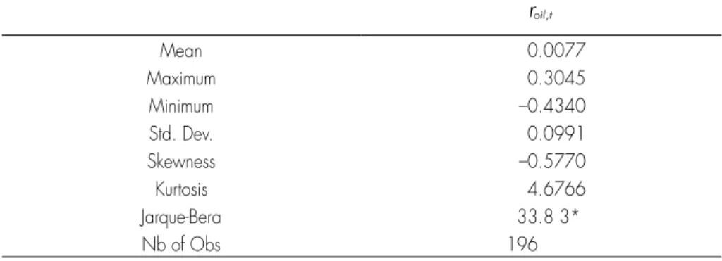
Standard descriptive statistics for return are reported in Table 1. They show evidence of

excess kurtosis and negative skewness. Not surprisingly, the Jarque-Bera test rejects the hypothesis of a Gaussian distribution. Some heteroscedasticity in the data may explain this non-normality as well as the presence of extremes (outliers). We do not explore the issue

of heteroscedasticity here as it is not our primary interest which is to model crude oil return conditional expectation and not higher moments.

Table 1 – Descriptive statistics for monthly crude oil returns (1993:12-2010:3)

roil t, Mean 0.0077 Maximum 0.3045 Minimum –0.4340 Std. Dev. 0.0991 Skewness –0.5770 Kurtosis 4.6766 Jarque-Bera 33.8 3* Nb of Obs 196

Note:(i) roil t, denotes crude oil return. It is computed as the price log differences. (ii) “*” denotes a rejection

of the null hypothesis of a Gaussian distribution at the 5% level.

In the empirical analysis presented in the next section, factors are extracted from a large panel of 187 macroeconomic and financial variables from developed and emerging countries. Our data set differs in its composition and time period from the widely known data set of Stock and Watson (2005) and its extension by Ludvigson and Ng (2009).12 _These two datasets mainly consist in U.S. data. As our aim is to include variables that are likely to influence crude oil return, we have included data from the main developed economies (128 variables) and also from emerging countries (59 variables). Therefore our dataset is representative of the world economy and high-level demand from emerging countries will be included in the information conveyed by estimated factors. These variables can also be classified into 103 real variables (73 for developed countries, 30 for emerging countries) and 84 nominal variables (55 for developed countries and 29 for emerging). For obvious reasons, we are constrained in our search of data for emerging countries but we try to make as much as possible a balanced panel. All data are extracted from DataStream. The list of these data is given in the appendix where a coding system indicates how the data were transformed so as to ensure stationarity. All of the raw data are standardized prior to estimation.

Following the analysis in Boivin and Ng (2006), we do not include as many variables as possible. Indeed, including too many variables may be particularly detrimental to the forecasting performance of the model. While we do not make any forecast in the present paper, we nevertheless pursue the logic of including a limited number of variables so as to render our study useful for future forecasting work. In addition, it is found in the empirical literature that including too many variables rarely lead to a better explanatory power. In a recent paper by Caggiano et al. (2011), the authors give a strong empirical support for

12. The original data set in Stock and Watson (2005) covers the period 1959:01 to 2003:12. It is slightly shortened in Ludvigson and Ng (2009) to cover the period 1964:01 to 2007:12.

the Euro area to the findings in Boivin and Ng (2006). Thinking that similar findings may be obtained for our world dataset, we limit the number of variables to be included in the computation of our static factors.

4. e

MpiricaliMpleMentation

4.1. Estimating the number of factors

We use Bai and Ng (2002) information criteria and Kapetanios (2010) sequential test to determine the number of factors. We briefly describe these two approaches and then present our results.

Bai and Ng (2002) information criteria are an extension to factor model of usual information criteria. If we note S k NT 1 iN1 Tt 1 xit ikFtk 2 m R R = − − = = t tl

t

_^

_h

_^

_h

_^

_h

_{the sum of squared residuals}

(divided by NT ) when k factors are considered, the information criteria have the following general expressions: , ) PCP ki

^

h

=S kt

^

h

+k g N Tvr2 i

^

h

, ln IC ki

^

h

= `S kt

^

h

j+kg N Ti

^

h

where _v

_r

2 _{is equal to S k} max

t

_^

_{h for a pre-specified value kmax and}

_{g N Ti}

_^

_,

_{h is a penalty}

function. We allow a maximum of kmax=20 factors and apply the four penalty functions , , 1, ,4

g N T ii

^

h

= f proposed by Bai and Ng (2002). The estimated number of factors

is chosen to minimize the aforementioned information criteria.

We also apply Kapetanios (2009) sequential test for determining the number of factors. This test is based on the property that if the true number of factors is k0, then, under some regularity conditions, the first k0 eigenvalues of the population covariance matrix R will increase at rate N while the others will remain bounded. If we denote by m

t

k,k=1,...,N

the N eigenvalues of the sample covariance matrix R, the difference m

t

k−m

t

kmax₊1 will tend to infinity for k=1,...,k0 but remain bounded for k k= +0 1,...,kmax where kmax is some

finite number such that k0<kmax. The null hypothesis that the true number of factors k0 is equal to k H k

^

0,k: 0=k

h against the alternative hypothesis

^

H k1,k: 0>k

h is therefore

tested with the test statistics m

t

k−m

t

kmax₊1. If there is no factor structure, m

t

_k−m

t

_kmax₊₁ properly

normalized by a sequence of constant

x

N T, should converge to a law limit. In the presence of factors, it should tend to infinity. The law limit as the rate of convergence

x

N T, have to be estimated by resampling technique. The test procedure is sequential. In a first step, we test

^

H k0,k: 0= =k 0

h against

^

H k >1,k: 0 0

h. If we reject the null hypothesis, then we

consider the null

^

H k0,k: 0= + =k 1 1

h. We stop once we cannot reject the null hypothesis.

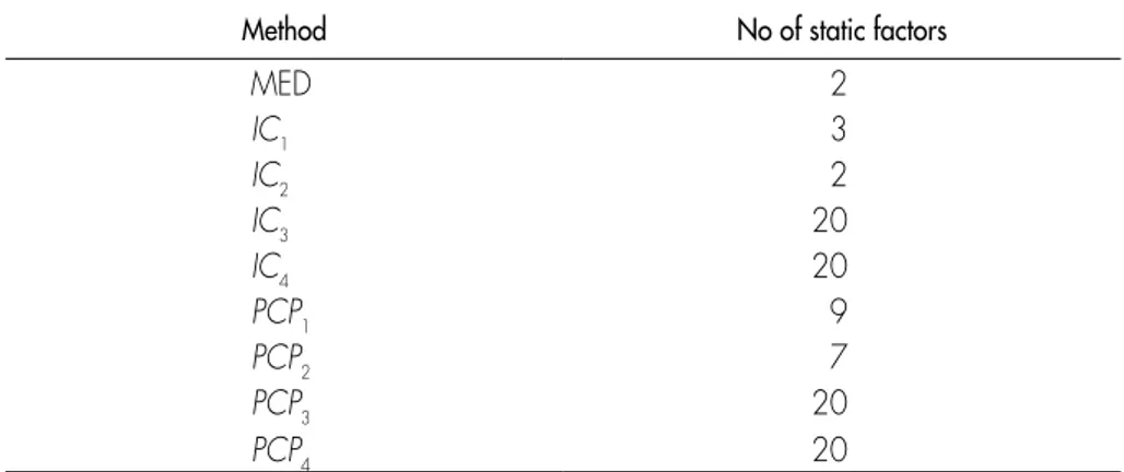
Kapetanios names this algorithm the MED (maximal eigenvalue distribution) algorithm. The estimated numbers of factors are displayed in Table 2. There is clearly no agreement on

that there is a great instability in determining the correct number of factors. According to Bai and Ng (2002) information criteria, the optimal number of factors runs from the 2 to 9. The Kapetanios test gives a number of 2 factors. Some information on the autocorrelation and the explanatory power of estimated factors Fttl are displayed in Table 3. We can note that the

first 3 factors only explain 20 % of the variance of the 187 data while we reach 36% with 9 factors. We decide to consider the set of the first 9 factors as potential set of regressors. Factors autocorrelations up to 3 lags also provided in Table 3 show that most factors appear

to be persistent.

Table 2 – Static factors selection results

Method No of static factors

MED 2 IC₁ 3 IC₂ 2 IC₃ 20 IC₄ 20 PCP₁ 9 PCP₂ 7 PCP₃ 20 PCP₄ 20

Notes: MED denotes the number of factors given by the Maximum eigenvalue algorithm. IC_i and PCP_i respectively denote the number of factors given by the information criteria IC and PCP estimated with penalty function g N Ti^ , h.

Table 3 – Summary statistics for Ft,ti for i = 1,...,9

factor i t1 t2 t3 Ri2 1 2 3 4 5 6 7 8 9 0.1614 0.1357 –0.0748 –0.0765 –0.2180 0.1801 0.0721 0.4086 –0.0066 0.1256 0.0805 0.0145 –0.0910 –0.0763 0.0388 0.2765 0.5013 –0.0305 0.3176 0.3110 –0.0294 0.1508 0.1213 0.0267 0.2744 0.3332 –0.0379 0.0975 0.1619 0.2030 0.2355 0.2654 0.2927 0.3185 0.3418 0.3636 Note: For i = 1,...,9, Ftit is estimated by the method of principal components using a panel of data

with 187 indicators of economic activity from 1993:12 to 2010:03 (196 time-series observations). The data are transformed (taking logs and differenced where appropriate) and standardized prior to estimation. ti denotes the i th autocorrelation. The relative importance of the common component, Ri2

4.2. Specification search

We now describe our specification search procedure. As a preliminary analysis, we regress crude oil return on each of the 9 factors and consider each R2 _{and Rr}2 _{as a measure of} the explanatory power of each individual factor. Results show that factor Ftt1 has the largest

explanatory power13 _{while factors 3 and 9 have almost none, so we exclude these latter} from our potential regressors. We consider all combinations of the 7 remaining factors and select the subset which minimizes the BIC criterion, as in Stock and Watson (2002) and Ludvigson and Ng (2009). According to this criterion, we choose the set of 4 factors

, , , F F F F F1 2 4 7

t= t t t tt t t t l

t

_^

_h

_{and estimate by OLS the following regression:}

roil t, = +a bF utt+ = +t a1 b1Ftt1+b2Ftt2+b4Ftt4+b7Ftt7+ut

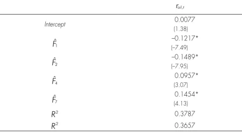
Our estimates are reported in Table 4.14 We explore a number of specifications where power

transformations of estimated factors are used as in Ludvigson and Ng (2009) to consider potential nonlinear effects. We do not report results here as nonlinear specifications have not a better explanatory power than linear ones.

Table 4 – OLS results for regression of the oil futures returns on selected factors

(1993:12 to 2010:03) roil t, Intercept 0.0077 (1.38) Ft1 –0.1217* (–7.49) Ft2 –0.1489* (–7.95) Ft4 0.0957* (3.07) Ft7 0.1454* (4.13) R2 _0.3787 R2 _0.3657

Notes: (i) t -statistics are reported in parenthesis under the estimates. A constant whose estimate is reported in the second row is always included in the regressions. (ii) For each test *, **, and *** respectively denotes rejection of the null hypothesis of no significant effect at the 1%, 5% and 10% levels.

13. Ftt1alone explains 14.3 % of the variation of crude oil return.

14. We add other possible extra explanatory variables (see Brown and Yücel (2008) for a justification for the case of natural gas). We add monthly stock/inventories changes computed as Dsit=log^S Si t,/ i t 1,−h where S,it stands for the stock level at date t (these data are extracted from the US Department of Energy website) and a dummy variable for the disruption in oil caused by Hurricanes Ivan in September 2004 and Katrina in August 2005. However these variables are not significant.

Each factor is significant and the R2 _{of the regression equals 37.87 % (the adjusted R}2 _is 36.57%) which is quite satisfying in light of the noisy nature of monthly returns. In addition, recall that we do not use oil price series which would increase the R2 _{as in Zagaglia} (2010) as they do not represent macro factors. However, it is not possible to interpret the sign of the estimated coefficients for the factors as the latter cannot be identified. In the next section, we present a simple method which could be used to give an interpretation of these factors.

4.3. Interpreting the estimated factors

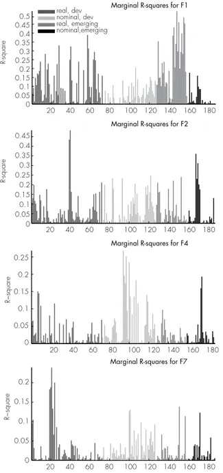
Ludvigson and Ng (2009) suggest a simple method to interpret the estimated factors. In practice, we regress each original variable on a single factor to measure the correlation between the former and the latter. Then, after sorting the variables along the horizontal axis say beginning with real variables and then with nominal variables, it is graphically possible to show the variables for which the highest R2 _{are obtained. The factor can then} be considered as representative of this set of variables. We classify our 187 series into four categories according to the characteristics real variable/nominal variable and developed countries/emerging countries. A finer classification would be difficult to illustrate and is relevant, in our opinion, only when a single country is at play.15 _{The R}2 _{from the regressions} of each of the 187 variables on each of the four factors F F F

t t t

t1, ,t2 t4 and F

t

t7 considered

separately are displayed on Figure 2.

Factor F

t

t1 can easily be interpreted as a real factor as it has its highest explanatory power for

real variables. To be more precise, F

t

t1 is mostly correlated with real variables from emerging

countries16_{. The correlation of F}

t1

t

_{with crude oil return can be interpreted as an evidence of}

the growing weight of emerging countries in oil imports during the time period considered. This finding is the most important result of the paper and it is new in the economic literature, to our best knowledge. Importantly, it may explain the rather weak support of previous studies to the common thinking that oil prices are mainly driven by speculative activity and not by real supply and demand variables.

Factor Ft4 reaches its highest explanatory power for nominal variables, especially for developed countries. It can therefore be interpreted as a “nominal” factor. Factors Ft7 and

Ft2 are more difficult to characterize as their explanatory power do not clearly cluster around a set of variables. Ft7reaches its highest explanatory power for a limited set of real variables from developed countries but no obvious interpretation can be given to Ft2.

Our results thus give a strong support to the theories in Hamilton (2009) and Kilian (2009) that emerging economies through an increasing demand for oil are responsible for the evolution of oil price in recent years. In particular, because we include in our database a

15. Ludvigson and Ng (2009) indeed rely on a finer classification but only use U.S. variables. We do not think that this methodology is applicable when several economies are considered if we want to preserve some interpretability. 16. Remind that factors are not identified, unless we impose some constraint to estimate them. Therefore the sign of the coefficient of Ftt1 in the crude oil return equation has no meaning per se.

number of Asian variables, it seems that their explanatory power is rather large and support the view in the literature of a demand-shock based-dynamics.

5. c

onclusion

This paper deals with the macroeconomic determinants of crude oil futures return taken at a monthly frequency. For such a purpose, we use the approximate factor model methodology along with a newly constructed database of macroeconomic and financial variables representative of developed and emerging countries. After investigating the optimal number of factors with several recent criteria from the econometric literature, we introduce the chosen estimated factors to explain the oil returns. Our results indicate that around 38% of the variability of oil futures return can be explained by a simple combination of 4 factors. These factors can be interpreted in light of their explanatory power of the variables included in the dataset. Importantly, we find that the first factor explaining oil price is strongly related to real variables from emerging countries. Hence, our first conclusion is that the analysis in Zagaglia (2010) is, as mentioned in Alquist et al. (2011), incomplete because the author only considers variables from the United-States of America. Our second, and more general conclusion is that, as commonly said in the financial press, emerging economies do influence oil price. While intuitive, this statement has not been supported in the literature so far. An exception is Faria et al. (2009, p. 793) where the authors show that “[...] Chinese growth can lead to an increase in oil prices that has a stronger impact on its export competitors”. Their results as well as ours provide a first step to the investigation of the relative share of emerging economies in driving oil prices.

The methodology used in the paper may be extended in a number of ways. In particular, as in Ludvigson and Ng (2010), it is possible to consider fully the fact that factors are estimated quantities that can be bootstrapped to make the analysis more robust. Ludvigson and Ng (2010) suggest a bootstrap procedure to deal with the issue of estimated factors. We do not think that the high explanatory power (and its related economic significance) of our main regression would be significantly modified but the robustness of the analysis would be enhanced. Dynamic factor models may also be used despite the misspecification issue discussed in the introduction. Indeed, if our interest is only in forecasting, as discussed below, the only barometer to choose among models will be the forecasting performance which may be better even with a misspecified model.

Figure 2 – Marginal R2 of macroeconomic and financial variables regressed on

the estimated factors no. 1, 2, 4 and 7

20 40 60 80 100 120 140 160 180 0.5 0.45 0.4 0.35 0.3 0.25 0.2 0.15 0.1 0.05 0 0.45 0.4 0.35 0.3 0.25 0.2 0.15 0.1 0.05 0 0.2 0.15 0.1 0.05 0 0.2 0.25 0.15 0.1 0.05 0 R-square

Marginal R-squares for F1 real, dev nominal, dev real, emerging nominal,emerging 20 40 60 80 100 120 140 160 180 R-square

Marginal R-squares for F2

20 40 60 80 100 120 140 160 180

R−square

Marginal R-squares for F4

20 40 60 80 100 120 140 160 180

R−square

Marginal R-squares for F7

Note: Each chart shows the R 2 _{from regressing the series number given on the x-axis onto each individual}

factor Fti. See the appendix for a description of the series. Series in the appendix are sorted as they appear in the Figure (real variables for developed countries, nominal variables for developed countries, real variables for emerging countries, nominal variables for emerging countries).

A natural extension of the present paper would be to investigate the forecasting power of time-series models based on large factors as those presented here. Forecasting crude oil price is of utmost importance for all international institutions, governments and multinationals. Nevertheless, as for exchange rates, the forecasting power of various methodologies that have been proposed in the literature is rather poor. Alquist et al. (2011) provide a very exhaustive survey of this challenging issue. The authors conclude that the random walk is not statistically beaten by any other method. To reach this conclusion, they compare the random walk forecasting accuracy with forecasts from futures prices (Wu and McCallum (2005), Alquist and Kilian (2010)), from exchange rates (Gilbert (1988), Chen et al. (2011)), from convenience yield predictions (Knetsch, 2007)17 _{and a number of time-series models based} on crude oil prices and other explanatory variables.

17. See also Gospodinov and Ng (2010) on the related issue of using the convenience yield to enhance inflation prediction.

r

eferences

Acharya, V.V., Lochstoer, L.A., Ramadorai, T. 2011. Limits to arbitrage and hedging: Evidence from commodity markets. NBER Working Paper no. 16875, March 2011, MA. Alquist, R., Kilian, L. 2010. What do we learn from the price of crude oil futures?, Journal of Applied Econometrics 25, 539-573.

Alquist, R., Kilian, L., Vigfusson, R.J. 2011. Forecasting the price of oil. In: G. Elliott and A. Timmermann, Handbook of Economic Forecasting, Elsevier, forthcoming.

Bai, J. 2003. Inferential theory for factor models of large dimensions, Econometrica 71, 135-172.

Bai, J., Ng, S. 2002. Determining the number of factors in approximate factor models, Econometrica 70, 191-221.

Bai, J., Ng, S. 2006. Confidence intervals for diffusion index forecasts and inference with factor-augmented regressions, Econometrica 74, 1133-1150.

Bai, J., NG , S. 2008. Large dimensional factor analysis, Foundations and Trends in Econometrics 3, 89-163.

Bartlett, M. S. 1951. The effect of standardization on a chi square approximation in factor analysis, Biometrika 38, 337-344.

Bekaert, G., Hodrick, R. 1992. Characterizing predictable components in excess returns on equity and foreign exchange markets, Journal of Finance 47, 467-509.

Bernanke, B., Boivin, J., Eliasz, P. 2005. Measuring the effects of monetary policy: A Factor-Augmented Vector Autoregressive (FAVAR) approach, Quarterly Journal of Economics 120, 387-422.

Boivin, J., NG, S. 2005. Understanding and comparing factor based forecasts, International Journal of Central Banking 1, 117-152.

Boivin, J., NG, S. 2006. Are more data always better for factor analysis, Journal of Econometrics 132, 169-194.

Borensztein, E., Jeanne, O., Sandri, D. 2009. Macro-hedging for commodity exporters, CEPR Discussion Paper, International Macroeconomics Series, no. 7513.

Borensztein, E., Reinhart, C.M. 1994. The macroeconomic determinants of commodity prices, IMF Staff Papers 41, 236-261.

Brown, S.P.A., Yücel, M.K. 2002. Energy prices and aggregate economic activity: An interpretative survey, Quarterly Review of Economics and Finance 42, 193-208.

Brown, S.P.A., Yücel, M.K. 2008. What drives natural gas prices?, Energy Journal 29, 45-60.

Büyükşahin, B., Haigh, M.S., Harris, J.H., Overdahl, J.A., Robe, M.A. 2009. Fundamentals, trader activity and derivative pricing, CFTC Working Paper.

Büyükşahin, B., Harris, J.H. 2011. Do speculators drive crude oil futures prices?, Energy Journal 32, 167-202.

Caggiano, G., Kapetanios, G., Labhard, V. 2011. Are more data always better for factor analysis? Results for the Euro area, the six largest Euro area countries and the UK, Journal of Forecasting 30, 736-752.

Chen, Y.-C., Rogoff, K.S., Rossi, B. 2010. Can exchange rates forecast commodity prices, Quarterly Journal of Economics 125, 1145-1194.

Faria, J.R., Mollick, A.V., Albuquerque, P.H., Léon-ledesma, M.A. 2009. The effect of oil price on China’s exports, China Economic Review 20, 793-805.

Forni, M., Hallin, M., Lippi, M., Reichlin, L. 2005. The generalized dynamic factor model, one sided estimation and forecasting, Journal of the American Statistical Association 100, 830-840.

Gilbert, C.L. 1989. The impact of exchange rates and developing country debt on commodity prices, Economic Journal 99, 773-784.

Gorton, G., Rouwenhorst, K.G. 2006. Facts and fantasies about commodity returns, Financial Analysts Journal 62, 47-68.

Gospodinov, N., Ng, S. 2010. Commodity prices, convenience yields, and inflation, Mimeo, Columbia University.

Hamilton, J.D. 2009. Causes and consequences of the oil shock of 2007-2008, Brookings Papers on Economic Activity Spring 2009, 215-261.

Kapetanios, G. 2010. A testing procedure for determining the number of factors in approximate factor models with large datasets, Journal of Business & Economic Statistics 28, 397-409.

Kaufmann, R.K. 2011. The role of market fundamentals and speculation in recent price changes for crude oil Energy Policy 39, 105-115.

Kilian, L. 2009. Comment on causes and consequences of the oil shock of 2007-2008, Brookings Papers on Economic Activity Spring 2009, 267-284.

Kilian, L., Vega, C. 2011. Do energy prices respond to U.S. macroeconomic news? A test of the hypothesis of predetermined energy prices, Review of Economics and Statistics 93, 660-671.

Knetsch, T.A. 2007. Forecasting the price of oil via convenience yield predictions, Journal of Forecasting 26, 527-549.

Lescaroux, F., Mignon, V. 2008. On the influence of oil prices on economic activity and other macroeconomic and financial variables, OPEC Energy Review 32, 343-380. Ludvigson, S.C., Ng, S. 2007. The empirical risk return relation: A factor analysis approach, Journal of Financial Economics 83, 171-222.

Ludvigson, S.C., Ng, S. 2009. Macro factors in bond risk premia, Review of Financial Studies 22, 5027-5067.

Ludvigson, S.C., Ng, S. 2010. A factor analysis of bond risk premia. In: A. Uhla and D.E.A. Giles, Handbook of Empirical Economics and Finance, Chapman & Hall, Boca Raton, FL. Parsons, J.E. 2010. Black gold and fool’s gold: Speculation in the oil futures market, MIT CEEPR WP 228.

Pindyck, R., Rotemberg, J. 1993. The comovement of stock prices, Quarterly Journal of Economics 108, 1073-1104.

Stock, J.H., Watson, M.W. 2002a. Forecasting using principal components from a large number of predictors, Journal of the American Statistical Association 97, 1167-1179. Stock, J.H., Watson, M.W. 2002b. Macroeconomic forecasting using diffusion indexes, Journal of Business and Economic Statistics 20, 147-162.

Stock, J.H., Watson, M.W. 2006. Forecasting with many predictors. In: G. Elliott, C.W.J. Granger, A. Timmermann (Eds.), Handbook of Economic Forecasting 1, Elsevier.

Tang, K., Xiong, W. 2011. Index investment and financialization of commodities, Mimeo, Stanford University.

Wheatley, S., 1989. A critique of latent variable tests of asset pricing models, Journal of Financial Economics 23, 325-338.

WU, T., MC CALLUM, A. 2005. Do oil futures prices help predict future oil prices?, Federal Reserve Bank of San Francisco Economic Letter, 2005-2038.

ZAGAGLIA, P. 2010. Macroeconomic factors and oil futures prices: A data-rich model, Energy Economics 32, 409-417.

a

ppendix

listofvariablesconsideredinthecoMputationofthecoMMonfactors Note: In the Trans column, we report the transformation used to make each variable stationary. ln denotes logarithm, ∆ ln and ∆² ln denote the first and second difference of the logarithm, lv denotes the level of the series, and ∆lv denotes the first difference of the series.

Developed countries

Series

Number Short name Mnemonic Trans Description Industrial production

1 IP: US USIPTOT G ∆ln US INDUSTRIAL PRODUCTION TOTAL INDEX VOLA _(2002=100) 2 IP: US USIPMFGSG ∆ln US INDUSTRIAL PRODUCTION MANUFACTURING _{(SIC) VOLA (1997=100)} 3 IP: Canada CNIPTOT.C ∆ln CN GDP INDUSTRIAL PRODUCTION CONN 4 IP: France FRIPMAN.G ∆ln FR INDUSTRIAL PRODUCTION MANUFACTURING _VOLA 5 IP: France FRIPTOT G ∆ln FR INDUSTRIAL PRODUCTION EXCLUDING _{CONSTRUCTION VOLA INDEX (2005=100)} 6 IP: Germany BDIPTOT G ∆ln BD INDUSTRIAL PRODUCTION INCLUDING _{CONSTRUCTION VOLA (2005=100)} 7 IP: UK UKIPTOT.G ∆ln UK INDEX OF PRODUCTION ALL PRODUCTION _{INDUSTRIES VOLA (2003=100)} 8 IP: UK UKIPMAN.G ∆ln UK INDUSTRIAL PRODUCTION INDEX _{MANUFACTURING VOLA (2003=100)} 9 IP: Japan JPIPTOT G ∆ln JP INDUSTRIAL PRODUCTION MINING & _{MANUFACTURING VOLA (2005=100)}

Orders and capacity utilization

10 Capacity utilization: _US USCUMANUG ∆lv US CAPACITY UTILIZATION MANUFACTURING VOLA 11 Manufct. new ord.: US USNOCOGMC ∆² _{ln US MANUFACTURERS NEW ORDERS CONSUMER}

GOODS AND MATERIALS CONN (base 1982) 12 Manufct. new ord.: US USBNKRTEQ ∆ln US MANUFACTURERS NEW ORDERS,NONDEFENSE _{CAPITAL GOODS SADJ (base 1982)} 13 New orders: Canada CNNEWORDB ∆ln CN NEW ORDERS: ALL MANUFACTURING _{INDUSTRIES (SA) CURA} 14 Manufct. ord.: _Germany BDNEWORDE ∆ln BD MANUFACTURING ORDERS SADJ (2000=100) 15 Manufct. ord.: Japan JPNEWORDB ∆ln JP MACHINERY ORDERS: DOM.DEMAND-PRIVATE _{DEMAND (EXCL. SHIP) CURA} 16 Operating ratio: Japan JPCAPUTLQ ∆lv JP OPERATING RATIO MANUFACTURING SADJ _(2005=100) 17 Business failures: Japan JPBNKRPTP ∆ln JP BUSINESS FAILURES VOLN

Housing start

Series

Number Short name Mnemonic Trans Description

19 Housing permits: _Canada CNHOUSE.O ln CN HOUSING STARTS: ALL AREAS (SA, AR) VOLA 20 Housing permits: _Germany BDHOUSINP ln BD HOUSING PERMITS ISSUED FOR BLDG.CNSTR.: _{BLDG.S-RESL, NEW VOLN} 21 Housing permits: _Australia AUHOUSE A ln AU BUILDING APPROVALS: NEW HOUSES CURN 22 Housing permits: Japan JPHOUSSTF ln JP NEW HOUSING CONSTRUCTION STARTED _VOLN

Car sales

23 Car registration: US USCAR P ln US NEW PASSENGER CARS TOTAL REGISTRATIONS _VOLN 24 Car registration: _Canada CNCARSLSE ln CN PASSENGER CAR SALES:TOTAL SADJ

25 Car registration: France FRCARREGP ln FR NEW CAR REGISTRATIONS VOLN 26 Car registration: _Germany BDRVNCARP ln BD NEW REGISTRATIONS CARS VOLN 27 Car registration: UK UKCARTOTF ln UK CAR REGISTRATIONS VOLN

28 Car registration : Japan JPCARREGF ln JP MOTOR VEHICLE NEW REGISTRATIONS: _{PASSENGER CARS EXCL.BELOW 66} Consumption

29 Consumer sentiment: _US USUMCONEH ∆ln US UNIV OF MICHIGAN CONSUMER SENTIMENT _{EXPECTATIONS VOLN (base 1966=100)} 30 Pers. cons. exp.: US USPERCONB ∆ln US PERSONAL CONSUMPTION EXPENDITURES (AR) _CURA 31 Pers. saving: US USPERSAVE ∆lv US PERSONAL SAVING AS % OF DISPOSABLE _{PERSONAL INCOME SADJ} 32 Retail sale: Canada CNRETTOTB ∆ln CN RETAIL SALES: TOTAL (ADJUSTED) CURA 33 Household confidence: _France FRCNFCONQ ∆lv FR SURVEY HOUSEHOLD CONFIDENCE INDICATOR _SADJ 34 Household confidence: _Germany BDCNFCONQ ∆lv BD CONSUMER CONFIDENCE INDICATOR _{GERMANY SADJ} 35 Retail sales: UK UKRETTOTB ∆ln UK RETAIL SALES (MONTHLY ESTIMATE, DS _{CALCULATED) CURA} 36 Household confidence: _UK UKCNFCONQ ∆lv UK CONSUMER CONFIDENCE INDICATOR UK SADJ 37 Retail sales: Australia AURETTOTT ∆ln AU RETAIL SALES (TREND) VOLA

38 Household confidence: _Australia AUCNFCONR ∆lv AU MELBOURNE/WESTPAC CONSUMER _{SENTIMENT INDEX NADJ} 39 Household expendi-_{ture: Japan} JPHLEXPWA ∆ln JP WORKERS HOUSEHOLD LIVING EXPENDITURE _{(INCL. AFF) CURN} 40 Retail sales: Japan JPRETTOTA ∆ln JP RETAIL SALES CURN

Wages and labor

41 Av. hourly real _{earnings: US} USWRIM D ∆ln US AVG HOURLY REAL EARNINGS _{MANUFACTURING CONA (base 82-84)}

Series

Number Short name Mnemonic Trans Description

43 Av. wkly hours : US USHKIM O ∆ln US AVG WKLY HOURS MANUFACTURING VOLA 44 Purchasing manager _{index: US} USPMCUE ∆ln US CHICAGO PURCHASING MANAGER DIFFUSION _{INDEX EMPLOYMENT NADJ} 45 Av. hourly real _{earnings: Canada} CNWAGES.A ∆ln CN AVG.HOURLY EARNINDUSTRIAL AGGREGATE _{EXCL. UNCLASSIFIED CURN} 46 Labor productivity: _Germany BDPRODVTQ ∆ln BD PRODUCTIVITY: OUTPUT PER MAN-HOUR _{WORKED IN INDUSTRY SADJ (2005=100)} 47 wages: Germany BDWAGES.F ∆ln BD WAGE & SALARY,OVERALL ECONOMY-ON A _{MTHLY BASIS(PAN BD M0191)} 48 Labor productivity: _Japan JPPRODVTE ∆ln JP LABOR PRODUCTIVITY INDEX -ALL INDUSTRIES SADJ

Unemployment

49 wages index: Japan JPWAGES E ∆ln JP WAGE INDEX: CASH EARNINGS ALL INDUSTRIES _SADJ 50 U rate: US USUNEM15Q ∆² ln US UNEMPLOYMENT RATE 15 WEEKS & OVER SADJ 51 U rate: US USUNTOTQ pc ∆² ln US UNEMPLOYMENT RATE SADJ

52 Employment: Canada CNEMPTOTO ∆² ln CN EMPLOYMENT CANADA (15 YRS & OVER, SA) _VOLA 53 U all: Germany BDUNPTOTP ∆ln BD UNEMPLOYMENT LEVEL (PAN BDFROM SEPT _{1990) VOLN} 54 U rate: UK UKUNTOTQ pc ∆² ln UK UNEMPLOYMENT RATE SADJ

55 Emp: Australia AUEMPTOTO ∆ln AU EMPLOYED: PERSONS VOLA 56 U all: Australia AUUNPTOTO ∆ln AU UNEMPLOYMENT LEVEL VOLA 57 U rate: Japan JPUNTOTQ pc ∆lv JP UNEMPLOYMENT RATE SADJ

International trade

58 Exports: US USI70 A ∆ln US EXPORTS CURN

59 Exports: EU EKEXPGDSA ∆ln EK EXPORTS TO EXTRA-EA17 CURN 60 Exports: France FREXPGDSB ∆ln FR EXPORTS FOB CURA

61 Exports: Germany BDEXPBOPB ∆ln BD EXPORTS FOB CURA 62 Exports: UK UKI70 A ∆ln UK EXPORTS CURN

63 Exports: Australia AUEXPG&SB ∆ln AU EXPORTS OF GOODS & SERVICES (BOP BASIS) _CURA 64 Exports: Japan JPEXPGDSB ∆ln JP EXPORTS OF GOODS CUSTOMSBASIS CURA 65 Imports: US USIMPGDSB ∆ln US IMPORTS F.A.S. CURA

66 Imports: EU EUOXT 09B ∆ln EU IMPORTS CURA 67 Imports: France FRIMPGDSB ∆ln FR IMPORTS FOB CURA

68 Imports: Germany BDIMPGDSB ∆ln BD IMPORTS CIF (PAN BD M0790) CURA 69 Imports: UK UKIMPBOPB ∆ln UK IMPORTS BALANCE OF PAYMENTS BASIS CURA 70 Imports: Australia AUIMPG&SB ∆ln AU IMPORTS OF GOODS & SERVICES (BOP BASIS) _CURA 71 Imports: Japan JPOXT009B ∆ln JP IMPORTS CURA

72 Terms of trade: UK UKTOTPRCF ∆ln UK TERMS OF TRADE EXPORT/IMPORT PRICES (BOP _{BASIS) NADJ} 73 Terms of trade: Japan JPTOTPRCF ∆ln JP TERMS OF TRADE INDEX NADJ

Series

Number Short name Mnemonic Trans Description 74 Money supply: US USM0 B ∆² ln US MONETARY BASE CURA 75 Money supply: US USM2 B ∆² ln US MONEY SUPPLY M2 CURA

76 Money supply: France FRM2 A ∆ln FR MONEY SUPPLY M2 (NATIONAL CONTRIBUTION _{TO M2) CURN} 77 Money supply: France FRM3 A ∆ln FR MONEY SUPPLY M3 (NATIONAL CONTRIBUTION _{TO M3) CURN} 78 Money supply: _Germany BDM1 A ∆ln BD MONEY SUPPLY-GERMAN CONTRIBUTION TO _{EURO M1(PAN BD M0790)} 79 Money supply: _Germany BDM3 B ∆ln BD MONEY SUPPLY-M3 (CONTRIBUTION TO EURO _{BASIS FROM M0195) CURA} 80 Money supply: UK UKM1 B ∆ln UK MONEY SUPPLY M1 (ESTIMATE OF EMU _{AGGREGATE FOR THE UK) CURA} 81 Money supply: UK UKM3 B ∆ln UK UK MONEY SUPPLY M3(ESTIMATE OF EMU _{AGGREGATE FORTHE UK) CURA} 82 Money supply: _Australia AUM1 B ∆ln AU MONEY SUPPLY M1 CURA

83 Money supply: _Australia AUM3 B ∆² ln AU MONEY SUPPLY M3 (SEE AUM3...OB) CURA 84 Money supply: Japan JPM1 A ∆ln JP MONEY SUPPLY: M1 (METHO-BREAK, APR. 2003) _CURN 85 Money supply: Japan JPM2 A ∆ln JP MONEY SUPPLY: M2 (METHO-BREAK, APR. 2003) _CURN 86 Credit: US USCOMILND ∆² ln US COMMERCIAL & INDUSTRIAL LOANS _{OUTSTANDING (BCI 101) CONA (base 2005)} 87 Credit: US USCILNNCB ∆lv US COMMERCIAL & INDL LOANS, NET CHANGE _{(AR) (BCI 112) CURA} 88 Credit: US USCRDNRVB ∆² ln US NONREVOLVING CONSUMER CREDIT _{OUTSTANDING CURA} 89 Credit: US USCSCRE Q ∆² ln US CONSUMER INSTALLMENT CREDIT TO _{PERSONAL INCOME (RATIO) SADJ} 90 Credit: France FRBANKLPA ∆² ln FR MFI LOANS TO RESIDENT PRIVATE SECTOR CURN 91 Credit: Germany BDBANKLPA ∆² ln BD LENDING TO ENTERPRISES & INDIVIDUALS CURN 92 Credit: UK UKCRDCONB ∆² ln UK TOTAL CONSUMER CREDIT: AMOUNT _{OUTSTANDING CURA} 93 Credit: Australia AUCRDCONB ∆² ln AU FINANCIAL INTERMEDIARIES: NARROW CREDIT _{PRIVATE SECTOR CURA} 94 Credit: Japan JPBANKLPA ∆² ln JP AGGREGATE BANK LENDING (EXCL. SHINKIN _{BANKS) CURN}

Stock index

95 Stock index: US USSHRPRCF ∆ln US DOW JONES INDUSTRIALS SHARE PRICE INDEX _{(EP) NADJ} 96 Stock index: France FRSHRPRCF ∆ln FR SHARE PRICE INDEX SBF 250 NADJ

97 Stock index: Germany BDSHRPRCF ∆ln BD DAX SHARE PRICE INDEX, EP NADJ

98 Stock index: UK UKOSP001F ∆ln UK FTSE 100 SHARE PRICE INDEXNADJ (2005=100) 99 Stock index: Japan JPSHRPRCF ∆ln JP TOKYO STOCK EXCHANGE TOPIX (EP) NADJ _(1968=100)

Series

Number Short name Mnemonic Trans Description Interest rate

100 Interest rate: US USFEDFUN ∆lv US FEDERAL FUNDS RATE (AVG.)

101 Interest rate: US USCRBBAA ∆lv US CORPORATE BOND YIELD MOODY’S BAA, _{SEASONED ISSUES} 102 Interest rate: US USGBOND ∆lv US TREASURY YIELD ADJUSTED TO CONSTANT _{MATURITY 20 YEAR} 103 Interest rate: France FRPRATE ∆lv FR AVERAGE COST OF FUNDS FOR BANKS / EURO _{REPO RATE} 104 Interest rate: France FRGBOND ∆lv FR GOVERNMENT GUARANTEED BOND YIELD (EP) _NADJ 105 Interest rate: Germany BDPRATE ∆lv BD DISCOUNT RATE / SHORT TERM EURO REPO _RATE 106 Interest rate: Germany BDGBOND ∆lv BD LONG TERM GOVERNMENT BOND YIELD 9-10 _YEARS 107 Interest rate: UK UKPRATE ∆lv UK BANK OF ENGLAND BASE RATE (EP)

108 Interest rate: UK UKGBOND ∆lv UK GROSS REDEMPTION YIELD ON 20 YEAR GILTS _{(PERIOD AVERAGE) NADJ} 109 Interest rate: Australia AUPRATE ∆lv AU RBA CASH RATE TARGET

110 Interest rate: Australia AUBOND ∆lv AU COMMONWEALTH GOVERNMENT BOND _{YIELD 10 YEAR (EP)} 111 Interest rate: Japan JPPRATE ∆lv JP OVERNIGHT CALL MONEY RATE, _{UNCOLLATERALISED (EP)}

112 Interest rate: Japan JPGBOND ∆lv JP INTEREST-BEARING GOVERNMENT BONDS _{10-YEAR (EP)} Exchange rate

113 Exchange rate: DM _{to US $} BBDEMSP ∆ln GERMAN MARK TO US $ (BBI) EXCHANGE RATE 114 Exchange rate: SK to _{US $} SDXRUSD ∆ln SD SWEDISH KRONOR TO US $ (BBI, EP) 115 Exchange rate: £ to $ UKDOLLR ∆ln UK £ TO US $ (WMR) EXCHANGE RATE 116 Exchange rate: Yen _{to $} JPXRUSD ∆ln JP JAPANESE YEN TO US $

117 Exchange rate: Aus.$ _{to US $} AUXRUSD ∆ln AU AUSTRALIAN $ TO US $ (MTH.AVG.) Producer price index

118 PPI: US USPROPRCE ∆ln US PPI FINISHED GOODS SADJ

119 PPI: Canada CNPROPRCF ∆ln CN INDUSTRIAL PRICE INDEX: ALL COMMODITIES _NADJ 120 PPI: Germany BDPROPRCF ∆ln BD PPI: INDL. PRODUCTS, TOTAL, SOLD ON THE _{DOMESTIC MARKET NADJ (2005=100)} 121 PPI: UK UKPROPRCF ∆ln UK PPI OUTPUT OF MANUFACTURED PRODUCTS _{(HOME SALES) NADJ} 122 PPI: Japan JPPROPRCF ∆ln JP CORPORATE GOODS PRICE INDEX: DOMESTIC _{ALL COMMODITIES NADJ}

Consumer price index

Series

Number Short name Mnemonic Trans Description 124 CPI: Canada CNCONPRCF ∆ln CN CPI NADJ

125 CPI: France FRCONPRCE ∆ln FR CPI SADJ 126 CPI: Germany BDCONPRCE ∆ln BD CPI SADJ

127 CPI: UK UKD7BT F ∆ln UK CPI INDEX 00 : ALL ITEMSESTIMATED PRE-97 _{2005=100 NADJ} 128 CPI: Japan JPCONPRCF ∆ln JP CPI: NATIONAL MEASURE NADJ

Emerging countries

129 IP: Brasil BRIPTOT G ∆ln BR INDUSTRIAL PRODUCTION VOLA index _2002=base 130 IP: China (cement) CHVALCEMH ∆ln CH OUTPUT OF INDUSTRIAL PRODUCTS CEMENT _VOLN 131 IP: India INIPTOT H ∆ln IN INDUSTRIAL PRODN. (EXCLUDING _{CONSTRUCTION & GAS UTILITY) VOLN index} 132 IP: India INIPMAN H ∆ln IN INDUSTRIAL PRODUCTION: MANUFACTURING _{VOLN index} 133 IP: Korea KOIPTOT.G ∆ln KO INDUSTRIAL PRODUCTION VOLA (2005=100) 134 IP: Mexico MXIPTOT H ∆ln MX INDUSTRIAL PRODUCTION INDEX VOLN 135 IP: Mexico MXIPMAN H ∆ln MX INDUSTRIAL PRODUCTION INDEX: _{MANUFACTURING VOLN}

136 IP: Philippines PHIPMAN F ∆ln PH MANUFACTURING PRODUCTION NADJ 2000 _prices 137 IP: South Africa SAIPMAN.G ∆ln SA INDUSTRIAL PRODUCTION (MANUFACTURING _{SECTOR) VOLA}

Orders and capacity utilization

138 Operating ratio: Brazil BRCAPUTLR ∆lv BR CAPACITY UTILIZATION MANUFACTURING NADJ 139 Mach. ord.: Korea KONEWORDA ∆ln KO MACHINERY ORDERS RECEIVEDCURN 140 Manufct. prod capa.: _Korea KOCAPUTLF ∆lv KO MANUFACTURING PRODUCTION CAPACITY _{NADJ (2005=100)}

Consumption

141 Retail sales: Korea KORETTOTF ∆ln KO RETAIL SALES NADJ (2005=100) Wages and labor

142 Labor cost: Brazil BRLCOST.F ∆ln BR UNIT LABOR COST NADJ Unemployment

143 U rate: Korea KOUNTOTQ pc ∆lv KO UNEMPLOYMENT RATE SADJ International trade

144 Exports: Brazil BREXPBOPA ∆ln BR EXPORTS (BOP BASIS) CURN 145 Exports: China CHEXPGDSA ∆ln CH EXPORTS CURN

146 Exports: India INI70 A ∆ln IN EXPORTS CURN 147 Exports: Indonesia IDEXPGDSA ∆ln ID EXPORTS FOB CURN

148 Exports: Korea KOEXPGDSA ∆ln KO EXPORTS FOB (CUSTOMS CLEARANCE BASIS) _CURN 149 Exports: Philippines PHEXPGDSA ∆ln PH EXPORTS CURN

Series

Number Short name Mnemonic Trans Description 150 Exports: Singapore SPEXPGDSA ∆ln SP EXPORTS CURN

151 Exports: Ta¨ıwan TWEXPGDSA ∆ln TW EXPORTS CURN

152 Imports: Brazil BRIMPBOPA ∆ln BR IMPORTS (BOP BASIS) CURN 153 Imports: China CHIMPGDSA ∆ln CH IMPORTS CURN

154 Imports: Indonesia IDIMPGDSA ∆ln ID IMPORTS CIF CURN

155 Imports: Korea KOIMPGDSA ∆ln KO IMPORTS CIF (CUSTOMS CLEARANCE BASIS) _CURN 156 Imports: Singapore SPIMPGDSA ∆ln SP IMPORTS CURN

157 Imports: Taïwan TWIMPGDSA ∆ln TW IMPORTS CURN

158 Terms of trade: Brazil BRTOTPRCF ∆ln BR TERMS OF TRADE NADJ (2006=100) 159 Money supply: Brazil BRM1 A ∆ln BR MONEY SUPPLY M1 (EP) CURN 160 Money supply: Brazil BRM3 A ∆ln BR MONEY SUPPLY M3 (EP) CURN

161 Money supply: China CHM0 A ∆ln CH MONEY SUPPLY CURRENCY IN CIRCULATION _CURN 162 Money supply: China CHM1 A ∆ln CH MONEY SUPPLY M1 CURN

163 Money supply: India INM1 A ∆ln IN MONEY SUPPLY: M1 (EP) CURN 164 Money supply: India INM3 A ∆ln IN MONEY SUPPLY: M3 (EP) CURN 165 Money supply: _Indonesia IDM1 A ∆ln ID MONEY SUPPLY: M1 CURN 166 Money supply: _Indonesia IDM2 A ∆² ln ID MONEY SUPPLYM2 CURN 167 Money supply: Korea KOM2 B ∆² ln KO MONEY SUPPLY M2 (EP) CURA

168 Money supply: Mexico MXM1 A ∆ln MX MONEY SUPPLY: M1 (EP) CURN base=end of _period 169 Money supply: Mexico MXM3 A ∆² ln MX MONEY SUPPLY: M3 (EP) CURN

170 Money supply: _Philippines PHM1 A ∆ln PH MONEY SUPPLY M1 (METHO BREAK AT 12/03) _CURN 171 Money supply: _Philippines PHM3 A ∆² ln PH MONEY SUPPLY M3 (METHO BREAK AT 12/03) _CURN 172 Money supply: Russia RSM2 A ∆² ln RS MONEY SUPPLYM2 CURN

Stock index

173 Stock index: Brazil BRSHRPRCF ∆² ln BR BOVESPA SHARE PRICE INDEX (EP) NADJ 174 Stock index: _Hong-Kong HKSHRPRCF ∆ln HK HANG SENG SHARE PRICE INDEX (EP) NADJ (31 _{july 1964 =100)}

Exchange rate

175 Exchange rate: Br.R. _{to US $} BRXRUSD ∆² ln BR BRAZILIAN REAIS TO US DOLLAR (AVG) 176 Exchange rate: Ch.Y. _{to US $} CHXRUSD ∆² ln CH CHINESE YUAN TO US DOLLAR (AVERAGE _AMOUNT) 177 Exchange rate: In.R. _{to US $} INXRUSD ∆² _{ln IN INDIAN RUPEES PER US DOLLAR (RBI)} 178 Exchange rate: Id.R. _{to US $} IDXRUSD ∆² ln ID INDONESIAN RUPIAHS TO US DOLLAR 179 Exchange rate: Mx.P. _{to US $} MXXRUSD ∆² ln MX MEXICAN PESOS TO US $-CENTRAL BANK _{SETTLEMENT RATE (AVG)}

Series

Number Short name Mnemonic Trans Description 180 Exchange rate: RS.R. _{to US $} RSXRUSD ∆² ln RS RUSSIAN ROUBLES TO US $ NADJ

Consumer price index

181 CPI: Brazil BRCPIGENF ∆² ln BR CPI GENERAL NADJ 182 CPI: China CHCONPRCF ∆ln CH CPI NADJ

183 CPI: India INCONPRCF ∆ln IN CPI: INDUSTRIAL LABOURERS (DS CALCULATED) _{NADJ (2001=100)} 184 CPI: Korea KOCONPRCF ∆ln KO CPI NADJ (2005=100)

185 CPI: Mexico MXCONPRCF ∆² ln MX CPI NADJ (JUN 2002=100) 186 CPI: Philippines PHCONPRCF ∆ln PH CPI NADJ