HAL Id: pastel-00957623
https://pastel.archives-ouvertes.fr/pastel-00957623
Submitted on 10 Mar 2014
HAL is a multi-disciplinary open access
archive for the deposit and dissemination of sci-entific research documents, whether they are pub-lished or not. The documents may come from teaching and research institutions in France or abroad, or from public or private research centers.
L’archive ouverte pluridisciplinaire HAL, est destinée au dépôt et à la diffusion de documents scientifiques de niveau recherche, publiés ou non, émanant des établissements d’enseignement et de recherche français ou étrangers, des laboratoires publics ou privés.
Genetic variation of growth and sex ratio in the
European sea bass (Dicentrarchus labrax L.) as revealed
by molecular pedigrees
Marc Vandeputte
To cite this version:
Marc Vandeputte. Genetic variation of growth and sex ratio in the European sea bass (Dicentrarchus labrax L.) as revealed by molecular pedigrees. Animal genetics. AgroParisTech, 2012. English. �NNT : 2012AGPT0057�. �pastel-00957623�
0
présentée et soutenue publiquement par
Marc VANDEPUTTE
le 4 octobre 2012
Genetic variation of growth and sex ratio in the European sea bass
(Dicentrarchus labrax L.) as revealed by molecular pedigrees
Doctorat ParisTech
T H È S E
pour obtenir le grade de docteur délivré par
L’Institut des Sciences et Industries
du Vivant et de l’Environnement
(AgroParisTech)
Spécialité : Génétique animale
Directrice de thèse : Edwige QUILLET
Jury
Mme Gabriele HÖRSTGEN-SCHWARK, Professeur, Université Georg-August, Göttingen Rapporteur
M. David PENMAN, Senior Lecturer, Université de Stirling Rapporteur
M. Philippe JARNE, Directeur de Recherches, CNRS Examinateur
M. Bernard CHEVASSUS-AU-LOUIS, Directeur de Recherches, INRA Examinateur
Mme Edwige QUILLET, Directrice de Recherches, INRA Examinatrice
ii
Remerciements
Il au a happ à pe so e ue le t a ail p se t da s e a us it est le sultat d u i estisse e t olle tif su plusieu s a es de t a ail. Qu il e soit do la ha e de p se te cela comme « ma » th se est à l ide e u e ha e i e se, a je pe se ue peu d tudia ts o t pu fi ie d u tel suppo t deu p ojets eu op e s su essifs… et d u e telle ua tit de données de qualité obtenues par un collectif hors normes.
Je souhaite tout d a o d remercier eu ui o t e ut au La o atoi e de G ti ue des Poisso s de l IN‘A e , pou a oi fait o fia e alo s u il faut ie di e u à ette po ue o e pe tise e g ti ue tait elati e e t l g e. Au sei de e la o atoi e, j ai pu t ou e u ad e e t ao di ai e pou d eloppe es o p te es, a e u tat d esp it o ie t e s les ésultats et l appli atio ui e a ja ais uitt , et ui est d ailleu s pou oi u e essit . E pa ti ulie , je souhaiterais remercier les « anciens » Bernard Chevassus, Edwige Quillet, René Guyomard et Daniel Chou out ui o t fait pa tage leu e périence sur tant de domaines différents.
E pa ti ulie , je suis t s e o aissa t à Ed ige Quillet d a oi a o pag tout au lo g de es a es a fo atio e g ti ue, d a o d e e ad a t lo s de o DEA e , puis e acceptant de suivrece travail de thèse malgré un agenda déjà plus que chargé. Merci pour ton attention bienveillante et ton exigence toujours constructive !
Merci aussi à Etienne Verrier pour avoir accepté de superviser cette thèse, en avoir assuré une construction conforme aux exigences académiques et un déroulement sans heurts.
Un grand merci également à Gabriele Hörstgen-Schwark, David Penman, Philippe Jarne et Bernard Chevassus d'avoir accepté de consacrer une part de leur temps à l'évaluation de ce travail.
La liste des person es a a t o t i u à l o te tio des sultats, à leu a al se et à leu ise e forme est longue, très longue, et si j e ou lie e tai s, u ils euille t ie e le pa do e … Je oud ais e pa ti ulie e e ie toute l uipe te h i ue de l If e e de Palavas, et en particulier Marie-Odile Vidal et F a çois ‘uelle sa s ui es poisso s e se aie t pas s et au aie t ja ais grandi. Merci aussi à tous ceux (à peu près toute la station de Palavas !) qui ont participé avec enthousiasme à de mémorables ha tie s de oise e t et de io t ies s tala t sou e t su plusieurs jours, sans faiblir et dans la bonne humeur. Evidemment, je veux adresser un merci tout spécial à Alain Vergnet, qui a été présent tout au long des ces expérimentations, se démenant pour que tout soit toujours organisé au mieux, pour améliorer les méthodes de collectes de données et t ou e des solutio s au p o l es ui o t pas ess de ous « stimuler », et aussi pour son humour subtil qui a toujours été un élément essentiel pour le moral des troupes sur ces expérimentations longues et il faut bien le dire parfois fastidieuses. Enfin, merci aussi à Marie-Jo Debos qui a toujours su trouver au plus vite les références bibliographiques les plus improbables. Quelle ha e d a oi e core une documentaliste !
La réalisation de ces travaux et la olle te de toutes es do es au ait pas o plus pu se fai e sa s la pa ti ipatio de eau oup de oll gues de l IN‘A ui o t fait a e ous le tou de la Méditerranée pour aller découper et mesurer des milliers de poissons dans des conditions parfois homériques avec des journées souvent peu conformes à la législation du travail ! Merci donc à Jean-Pierre Hiseux, Lucas Lefèvre, Elisabeth Perrot, Caroline Hervet, Amandine Launay, Nicolas Dechamp,
iii
Nicolas Collanges, Olivier Merdy,... et à Mathilde Dupont-Nivet qui non seulement a « mis les mains dedans » à de o euses ep ises ais e plus a a al s , dis ut , dig …toute la pa tie su la croissance lui doit beaucoup !
Ce travail ne se serait pas fait non plus sans nos partenaires privés, français et étrangers, qui ont pris part aux deux projets européens successifs. Au-delà des structures, je voudrais remercier personnellement Hervé Chavanne, qui a eu la folie de mettre en place en pratique un plan de oise e t o e pe so e a ait os l i agi e hez le a , et Glen Pagelson, André Bravo, Joana Amaral, Pedro Marques, Carlos Mazzorra, Rémi Ricoux et Stanislas Laureau, sans oublier Pierrick Haffray et Cedric Pincent du Sysaaf, pour leur enthousiasme, leur endurance, leur organisation et leu se s de l hospitalité qui font ue ous eg etto s tous aujou d hui es e p i e tatio s u peu folles.
Et puis ie sû , ie de tout ela au ait t possi le sa s B at i e Chatai , ui a oulu e programme, a toujours cru que nous y arriverions, a su entraîner toute cette fine équipe, trouver les o e s de fai e o te e t e ui tait au d ut u u e id e u peu hi i ue o ous l a ie fait sa oi … et a o attu les l e ts a e u e e gie sa s faille. Quelle ha e ue de fi ie du soutie et de l a iti d u e « légende vivante » de l a ua ultu e du a ! Béatrice, ette th se est aussi u peu la tie e…
iv
"Ondine scrute l'océan où sa mère doit..., où son père doit chasser le congre ou le bar. Le congre que le bar abhorre ou le bar que le congre hait. Car Ondine a la dalle et la mère a les crocs. Selon qu'il aura pris la barque à bars ou la barque à congres, le père devra remplir la barque à bars à ras bord de bars ou la barque à congres à ras bord de congres. Or, il n'a pas pris la barque à congres ; Il a pris la barque à bars. A l'arrière plan, le spectateur voit, au flanc de la montagne rouge feu, moutonner un maquis vert. Il y serpente des chemins rares qui débouchent soudain sur des criques sauvages où nul imbécile, cintré dans sa bouée Snoopy ne vient jamais ternir de son ombre grasse et populacière, l'irréelle clarté des fonds marins mordorés, où s'insinue le congre que donc, le bar abhorre. Oui : le bar abhorre le congre par atavisme. Le congre est barivore. Et donc le bar l'abhorre. Le bar est fermé aux congres du même fait que le palais des congres est ouvert au bar."
Pierre Desproges, 1986
v
Financial and technical support
Genetic parameters estimation experiment (Chapter 2)
This work was carried out in the framework of a CRAFT project no. Q5CR-2002-71720 (Heritabolum) funded by the EC and the private farms, Panittica Pugliese (Torre Canne di Fasano, Italy), Viveiro Villanova (Vila Nova de Milfontes, Portugal) and Ardag Red sea Maricultrure (Eilat, Israel) which are also thanked for their active participation, especially Hervé Chavanne, André and Joana Bravo and Glen Pagelson. Authors are also grateful to Stanislas Laureau from Ecloserie Marine de Gravelines (France) which helped us organizing the mating design., and the technical staff from Ifremer (Alain Vergnet, Marie-Odile Vidal, François Ruelle) is warmly thanked for taking care of the fish and organizing measurements over the two years of the experiment.
Response to selection experiment (Chapter 3)
This work was done in the frame of the COMPETUS project, funded by Ardag Red Sea Mariculture (Eilat, Israel), Ecloserie Marine de Gravelines (Gravelines, France), Les Poissons du Soleil (Balaruc, France), Tinamenor SA (Pesues, Cantabria, Spain), Viveiro Vilanova (Vila Nova de Milfontes, Portugal) and the European Union (project COOP-CT-2005-017633). I wish to express my gratitude to Massimo Caggiano from Panittica Pugliese (Torre Canne, Italy), which gave access to the cryopreserved sperm from the base wild population and from the PROSPER-like selected population.
The p ese t o k as also pa t of the p og a e of the ‘esea h G oup A lio atio G ti ue des Poisso s et ee financed by INRA and Ifremer (2004-2008)
vi
Table of contents
1
General introduction _____________________________________________________ 1
1.1 Aquaculture: a fast-growing animal production deserving optimisation______________ 1 1.2 Starting from the wild: domestication and selective breeding in fish ________________ 2 1.3 Selective breeding in fish: accessing the pedigree? ______________________________ 4
1.3.1 Not using the pedigree: individual selection ___________________________________________ 4 1.3.2 Separate rearing of the families _____________________________________________________ 5 1.3.3 A posteriori parentage assignment with genetic markers _________________________________ 6 1.4 The genetics of European sea bass ___________________________________________ 7
1.4.1 Population genetics of sea bass _____________________________________________________ 7 1.4.2 Genetic variation for quantitative traits _______________________________________________ 8
1.5 Sex ratio in the sea bass: a difficult trait to deal with _____________________________ 8 1.6 A two-steps approach for studying genetic variation and its application to sea bass culture 10
2
Genetic variation as revealed by between-family variation in common garden
experiments ______________________________________________________________ 15
2.1 Genetic variation for body size _____________________________________________ 15
2.1.1 Introduction ____________________________________________________________________ 15 2.1.2 Material and methods ____________________________________________________________ 16 2.1.2.1 Animals ___________________________________________________________________ 16 2.1.2.2 Data collection. _____________________________________________________________ 17 2.1.2.3 Parentage assignment _______________________________________________________ 17 2.1.2.4 Statistical analyses __________________________________________________________ 18 2.1.3 Results ________________________________________________________________________ 19 2.1.4 Discussion _____________________________________________________________________ 22 2.1.4.1 Deformities ________________________________________________________________ 22 2.1.4.2 Maternal effect _____________________________________________________________ 22 2.1.4.3 Heritability estimates ________________________________________________________ 23 2.1.4.4 Genotype by environment interactions _________________________________________ 23 2.1.4.5 Correlations between growth traits ____________________________________________ 24 2.1.5 Summary ______________________________________________________________________ 26
2.2 Genetic variation for growth rate ___________________________________________ 27
2.2.1 Introduction ____________________________________________________________________ 27 2.2.2 Material and methods ____________________________________________________________ 27 2.2.2.1 Animals ___________________________________________________________________ 27 2.2.2.2 Data collection _____________________________________________________________ 28 2.2.2.3 Statistical analyses __________________________________________________________ 29 2.2.3 Results and discussion ____________________________________________________________ 30 2.2.4 Summary ______________________________________________________________________ 32
2.3 Additional data: genetic correlations between initial weight, slaughter weight and growth rate 32
vii
2.4.1 A polygenic hypothesis for sex determination _________________________________________ 35 2.4.1.1 Introduction _______________________________________________________________ 35 2.4.1.2 Material and methods _______________________________________________________ 36 2.4.1.3 Results ____________________________________________________________________ 39 2.4.1.4 Discussion _________________________________________________________________ 41 2.4.1.5 Summary __________________________________________________________________ 45 2.4.2 Supplemental information ________________________________________________________ 46 2.4.2.1 The threshold model for sex determination ______________________________________ 46 2.4.2.2 Genetic and environmental correlations of sex tendency and body length at different ages 47
3
Effects of domestication and directional selection for body length _______________ 48
3.1 Selection response for growth ______________________________________________ 48
3.1.1 Introduction ____________________________________________________________________ 48 3.1.2 Materials and methods ___________________________________________________________ 49 3.1.2.1 Selection of sires____________________________________________________________ 49 3.1.2.2 Constitution of the experimental progeny _______________________________________ 50 3.1.2.3 Rearing conditions and phenotyping ____________________________________________ 51 3.1.2.4 Parentage assignment _______________________________________________________ 51 3.1.2.5 Statistical analyses __________________________________________________________ 52 3.1.3 Results ________________________________________________________________________ 53 3.1.3.1 Parentage assignment _______________________________________________________ 53 3.1.3.2 Selection response in separate tanks ___________________________________________ 54 3.1.3.3 Selection response in mixed tanks______________________________________________ 55 3.1.4 Discussion _____________________________________________________________________ 57 3.1.4.1 Parentage assignment in mixed tanks ___________________________________________ 57 3.1.4.2 Response to selection _______________________________________________________ 57 3.1.4.3 Effect of domestication ______________________________________________________ 59 3.1.4.4 Possible application of the results at commercial scale _____________________________ 59 3.1.5 Summary ______________________________________________________________________ 60
3.2 Selection response for sex ratio _____________________________________________ 61
3.2.1 A necessary baseline: sex ratios in wild sea bass populations_____________________________ 61 3.2.1.1 Introduction _______________________________________________________________ 61 3.2.1.2 Material and methods _______________________________________________________ 62 3.2.1.3 Results ____________________________________________________________________ 62 3.2.1.4 Discussion _________________________________________________________________ 63 3.2.1.5 Summary: _________________________________________________________________ 66 3.2.2 Sex ratio changes in domesticated and selected populations _____________________________ 67 3.2.2.1 Introduction _______________________________________________________________ 67 3.2.2.2 Material and methods _______________________________________________________ 68 3.2.2.3 Results ____________________________________________________________________ 69 3.2.2.4 Discussion _________________________________________________________________ 69 3.2.2.5 Summary __________________________________________________________________ 71 3.2.3 Additional data: genetic correlation of growth and sex tendency over time _________________ 72
3.3 Modelling the mid-term evolution of growth and sex ratio in farmed sea bass populations under selection for growth _______________________________________________________ 74
3.3.1 Why model the evolution of sex ratio under selection for growth ? _______________________ 74 3.3.2 A stochastic simulation model _____________________________________________________ 75 3.3.3 Parameters tested _______________________________________________________________ 76
viii
3.3.4 Results and discussion ____________________________________________________________ 77
4
General Discussion _____________________________________________________ 79
4.1 Summary of the main results _______________________________________________ 79 4.2 A perspective for sea bass domestication and breeding programmes _______________ 82
4.2.1 A proof of concept of the use of marker-based parentage assignment _____________________ 82 4.2.2 Selection for increased body weight ________________________________________________ 86 4.2.3 Genotype by environment interactions for growth: which consequences? __________________ 91 4.2.4 Practical consequences of genetic variation for sex ratio ________________________________ 93 4.2.5 How to move towards monosex female sea bass populations? ___________________________ 96
4.3 An evolutionary perspective on the genetic variation of sex ratio in sea bass, and its relations with growth __________________________________________________________ 101
4.3.1 Polygenic sex determination: a very peculiar system ? _________________________________ 101 4.3.2 The adaptive significance of polygenic sex determination (in sea bass) ____________________ 105 4.3.3 Sex determination and sex differentiation? __________________________________________ 109
4.4 Conclusion _____________________________________________________________ 112
1
1 General introduction
1.1 Aquaculture: a fast-growing animal production deserving optimisation
In historic times, the sea has always been considered as an inexhaustible source of high quality food for humanity. It is only very recently that it became more and more evident that this was not the case. When FAO records on capture fisheries started in 1951, 70 % of the world fisheries were considered undeveloped, and less than 10% were fully exploited, while in 1999 the picture was quite the opposite: 50% of the fisheries were fully exploited, and more than 40% were overfished or collapsed (Froese and Kesner-Reyes, 2002). This can also be seen in the production curve, where growth of fisheries production has stopped and is even declining since the 80's despite a continuous increase in fishing effort (FAO, 2009). Nowadays, although propositions are done by scientists to help better manage capture fisheries (e.g. Pauly et al., 2002), nobody seriously expects that world capture fisheries production will ever produce more than they did in the 1980's, and some authors argue that capture fisheries could even completely collapse by the middle of the 21th century (Worm et al., 2006).
Facing this rise and fall of capture fisheries, the demand for seafood has continuously increased, and indeed the total world production of fish1 has never stopped growing since 1950 (FAO, 2009). Where does the difference come from? It comes from aquaculture, which is the fastest growing animal production in the world for more than 20 years (Figure 1-1). Aquaculture became more important than sheep and goats in the 1990s, and is now catching up with bovine meat and
eggs production. When compared with capture fisheries, aquaculture now provides ca. 50% of the human consumption of fish (FAO, 2009). Thus, all the increase in fish production at the world level since the 1980's comes from aquaculture. This has to be mitigated by the fact that the bulk of aquaculture production comes from Asia, with 60-70% of the production originating from just China. Consequently, the world production trend may not be the same in all countries, and especially in Europe, the growth of the production is much slower. Still, in addition to significant inland productions like common carp (Cyprinus carpio) in Central Europe or rainbow trout (Oncorhynchus
mykiss) all over Europe, there are some success stories. These are mainly marine aquaculture, -
another difference with the global situation where freshwater aquaculture dominates. These successful European species are Atlantic salmon (Salmo salar) in Northern Europe, European sea bass (Dicentrarchus labrax) and gilthead sea bream (Sparus aurata) in the Mediterranean area. The
1 in this section, the generic term "fish" represents finfish, mollusks and crustaceans.
Figure 1-1: World production of farmed animal products (except milk)
since 1960 (FAOSTAT data) 0.E+00 2.E+07 4.E+07 6.E+07 8.E+07 1.E+08 1.E+08 1960 1980 2000 2020 W or ld a nn ua l pr od uc ti on (t ) Eggs Bovine meat Poultry meat Sheep and Goats meat Aquaculture (w/o algae) Pig meat
2
methods to rear those last two species were developed only in the mid 80's, and since then the production of each of them has grown to more than 130,000t/year in 2008 (FEAP, 2008).
This very fast growth of aquaculture inevitably raises questions about its sustainability. Important concerns were raised about the use of fish meal and fish oil, originating from small pelagic fisheries (especially in Peru and Chile) in the aquaculture of carnivorous fishes. Some estimations of the global efficiency of the system led to the conclusion that aquaculture was not producing more fish, but indeed increased the pressure on wild fish stocks (Naylor et al., 2000). However, the composition of fish feeds is evolving quickly with inclusion of more and more oils and proteins from plant origin, and provided this trend continues, feed source is not seen as a major threat to the sustainability of aquaculture production anymore (Tacon and Metian, 2008; Naylor et al., 2009).
Selective breeding has been shown to be a major driver in the improvement of production efficiency in terrestrial species. In broiler chickens for example, it has been shown that selective breeding was responsible for more than 80% of the increase in growth rate observed between 1957 and 2001 (Havenstein et al., 2003b). The same experiment also revealed an improvement in feed conversion ratio (1.62 in the selected strain vs. 2.14 in the control strain) and in meat yield (breast yield at 71 days: 21.3% in the selected strain, vs. 11.0% in the control strain - Havenstein et al., 2003a). Such important productivity improvements have also been seen in almost all terrestrial livestock species (reviewed in Van Der Steen et al., 2005), with a correlated improvement in production efficiency allowing a reduced production of greenhouse gases per ton of animal product (Hume et al., 2011). Therefore, it can be reasonably forecast that genetic improvement also has potential to dramatically increase the productivity and efficiency of aquaculture production. This is of crucial importance as aquaculture will play an ever-increasing role in the production of aquatic products at the world level.
1.2 Starting from the wild: domestication and selective breeding in fish
A major difference between terrestrial livestock and aquaculture species is their domestication status. In terrestrial livestock, the bulk of the production (>90% in volume2) is based on four species, pig (Sus scrofa domesticus), chicken (Gallus domesticus), cattle (Bos taurus) and sheep (Ovis aries). All those species are long domesticated, between 10000 and 1500 years before present (reviewed in Mignon-Grasteau et al., 2005). It should be noted that domestication involves an evolutionary process by which animal populations become adapted to man and the environment he provides, in addition to environment induced ontogenic changes at the level of the animal itself (Price, 1984). For this reason, only species which went through many generations of captive breeding can be considered domesticated.
In the case of fish, the two species considered domesticated are the common carp and the goldfish
Carassius auratus (Balon, 2004), both domesticated at the end of the Middle Ages. The real
possibility to domesticate other species arose with the discovery of artificial fertilization of salmonids in the 17th century (Coste, 1853). However, in many important species for aquaculture, the life cycle has been completely closed (by controlled reproduction of captive-born fishes) only very recently. In salmon for example, this occurred in the 1970's, thus leading to ca. 10 generations of captive breeding until 2010. In the European sea bass and the gilthead sea bream, the techniques for captive reproduction and efficient larval rearing were only established in the mid-1980's, but this does not ensure a domestication of those species, as many hatcheries still use wild broodstock. Moreover,
3
even hatcheries which conduct breeding programmes on these species were only between 3 and 5 generations from the wild in 2009 (Chavanne, pers.comm.).
Domestication of fish is expected to increase the adaptation of fish lines to the farming environment, producing bolder animals, with increased motivation for food, losing anti-predator and reproductive behaviour (reviewed in Ruzzante, 1994; Gross, 1998; Vandeputte and Prunet, 2002). As one of the main determinants of domestication is "natural selection" for the captive environments, it can be foreseen that domestication may act very rapidly in fish species, where fertility is very high (up to 106 eggs/kg female weight in many species), as the intensity of this natural selection may be very high (Doyle, 1983; Doyle et al., 1995). Thus, domesticating fish is a first step towards farmed fish lines which has proven very efficient: when comparing wild and domesticated rainbow trout, after a few tens of generations of captive breeding, the difference in growth rate between the offspring of domesticated and wild trout lines is spectacular (from ca. x2 to x27 for body weight at a given age -Devlin et al., 2001; Morkramer et al., 1985). In Coho salmon Oncorhynchus kisutch, domestication has also been shown to increase growth rate after four generations, although to a lesser extent (Hershberger et al., 1990).
The next step of genetic improvement following domestication is selective breeding for one or several traits of interest. Indeed, as we indicated before that in most fish species domestication is very recent, most of the time, unlike what happened in livestock, selective breeding starts as soon as the life cycle is closed. The reason for this is that the theory of breeding and the gains it can generate is well known, which was not the case for cattle 10,000 years ago! The first trait to be selected is always growth rate, which has the advantage to be easily measured and to give a visible result. The result is important genetic gains in growth rate in many species, in the range of 9-20% per generation as reviewed by Gjedrem and Thodesen (2005). More recent results are in the same range: 21.5% per generation in brown trout (Chevassus et al., 2004), 7.1-18.7% in Nile tilapia Oreochromis niloticus (Khaw et al., 2008; Thodesen et al., 2011) and 10.2-13.9% in Coho salmon (Neira et al., 2006).
These successful achievements are the consequence of 1) the relatively high heritability of body weight in fish (mostly between 0.20 and 0.50 - see review by Gjedrem and Olesen, 2005), 2) the high coefficient of variation of body weight (20-35% vs. 7-10% in land animals - Gjedrem, 1998) and 3) the possible use of high selection intensities, due to the high fertility and small individual size of fish.
Heritability has been estimated for a number of other traits like reproduction traits, processing yields, body shape, fat content, disease resistance,... and in most cases significant genetic variation can be identified, allowing the development of breeding programmes on virtually any trait (see Gjedrem and Olesen, 2005, for a general review, Quillet et al., 2007 and Odegard et al., 2011 for reviews focused on disease resistance traits).
Altogether, we can conclude that like in terrestrial livestock, and probably even more owing to the high possible selection intensities, domestication and selection have the potential to be major contributors to the development of efficient aquaculture industries throughout the world.
4
1.3 Selective breeding in fish: accessing the pedigree?
An important point, in any optimized selective breeding programme, is the capability to keep track of the pedigree. The knowledge of the pedigree has three main interests:
allowing a better management of inbreeding, as with a known pedigree inbreeding can be calculated and constrained through optimized matings;
permitting the estimation of heritability and genetic correlations through the evaluation of the within and between-family variance components for the trait(s) of interest, a strategy much more efficient than realized heritability, which is limited to one trait and requires a selected and a control line;
setting up more efficient breeding programmes using family information as a means to improve the precision of the selection index.
In fish, knowledge of the pedigree is complicated by the fact that hatchlings are very small in size (from a few tens of micrograms to 150 mg) and cannot be physically tagged. There are three ways to solve the issue of using pedigrees in fish breeding programmes: (i) not use them (which is the case with mass or individual selection), (ii) use separate rearing of progenies until they reach a size where they can be tagged (usually ca. 20g mean body weight) or (iii) use genotyping of polymorphic markers to assess the parentage of individuals.
1.3.1 Not using the pedigree: individual selection
Using individual selection can yield interesting gains owing to the high selection intensity possible, and remains a choice of interest for selecting traits that can be measured directly on live breeding candidates. This method produced positive results selecting for body weight in channel catfish
Ictalurus punctatus (Dunham and Smitherman, 1983), gilthead sea bream (Knibb et al., 1998), Nile
tilapia (Basiao and Doyle, 1999), brown trout (Chevassus et al., 2004) and common carp Cyprinus
carpio (Vandeputte et al., 2008). However, this was not always the case, and unsuccessful trials in
common carp (Moav and Wohlfarth, 1976) and Nile tilapia (Teichert-Coddington and Smitherman, 1988; Huang and Liao, 1990) initially led some to think that selection was not operating in fish (Gjedrem, 2012). It was also the rationale to develop the P ospe ethod, a opti ized i di idual selection method for growth that proposes to control non genetic maternal effects and competition effects (Chevassus et al., 2004) and has been the basis of the development of many breeding programmes in France (Haffray et al., 2004; Vandeputte et al., 2009a).
Other traits have also been successfully selected for by mass selection, like body shape in common carp (Ankorion et al., 1992) and muscle fat content, estimated with a Distell Fat-meter, in rainbow trout (Quillet et al., 2005).
Individual selection has the advantage that it is the easiest and cheapest to implement of selection methods, making it particularly suitable for small or medium companies. However, it also suffers from serious drawbacks. The first one is that this method is likely to generate important rates of inbreeding if not properly managed (Gjerde et al., 1996; Dupont-Nivet et al., 2006). Second, it cannot be used on traits that cannot be recorded (directly or indirectly) on the live breeding candidates. In addition, the genetic parameters of the traits selected remain generally unknown. Realized heritability for the selected trait can be estimated if a control line is maintained in parallel, but this is a rough estimate of the true heritability, and most of all the genetic parameters of other potentially
5
interesting traits (and the genetic correlations among those) will remain unknown unless specific selection experiments for these traits are set up. Finally, selection might be more effective, especially with low heritability traits, if family information can be used (Falconer and Mackay, 1996). This will be especially true when selection applies to a combination of several traits - and it is a normal fate for breeding programmes to incorporate more traits over time.
1.3.2 Separate rearing of the families
Family-based selection with separate rearing of progenies is the method which has been used and developed in the first "modern" breeding programmes for fish in the 1970's-1980's in Norway (Gjedrem, 2010, 2012) and in North America (e.g. Hershberger et al., 1990). Typically, in such breeding programmes, each male is mated with 2-3 females in a hierarchical system, then progenies are reared separately until tagging (100-400 separate rearing units needed). After tagging3 at ca. 20g (almost 1 year in Atlantic salmon - Gjerde et al., 1994), some breeding candidates remain on the breeding site, while other tagged fish from the different families are sent to on-farm growing tests or to challenge testing for diseases (Gjedrem, 2010). This type of breeding programme was then extended to other species, with famous programmes like the GIFT (Genetically Improved Farm Tilapia) in the Philippines (Eknath and Acosta, 1998), the programme for the improvement of rohu
Labeo rohita in India (Gjerde et al., 2005) or several programmes for the Pacific white shrimp Penaeus vannamei (e.g. Gitterle et al., 2005).
Knowledge of the multi-generational pedigree allows the use of optimal methods, like BLUP (Best Linear Unbiased Prediction) for the prediction of breeding values. Undoubtedly, such breeding programmes have generated the bulk of the genetic gain in the major genetically improved species of world aquaculture like Nile Tilapia, Atlantic salmon and Pacific white shrimp (Neira, 2010; Rye et
al., 2010). While they are very convenient to include traits recorded on sibs in challenge tests
(including farm ongrowing data), the initial rearing phases are done in conditions that differ a lot from industry standards, owing to the necessity to have all families reared separately in small volume tanks or hapas. A fish that starts its life at a few milligrams (or tens of milligrams in the case of salmonids) has already increased its body weight by a factor of 200 to 2000 when it reaches 20g, while the way to commercial weight only implies a further multiplication by a factor of 20 to 200.
Therefore, common environment effects (= "tank effects") are expected to be large, and indeed they may be so when measured: 10-30% of the phenotypic variance for body weight in common carp (Ninh et al., 2011), a "substantial" amount in rohu carp (Gjerde et al., 2005), from 2 to 20% in Atlantic Salmon (Gjerde et al., 1994), from 3 to 12% in Atlantic cod Gadus morhua (Gjerde et al., 2004; Tosh
et al., 2010), 14-17% in rainbow trout (Henryon et al., 2002). In some cases however, it appears that
tank effects are contained to limited level (0 to 9% of phenotypic variance in rainbow trout- Elvingson and Johansson, 1993). High tank effects are problematic as they may bias the estimated family values, and then the estimated breeding value of individuals. In addition to this, the need to minimize family (and then rearing units) number tends to promote hierarchical mating designs, as for a given effective population size (needed to avoid inbreeding) they imply the production of less families than most factorial mating designs. However, hierarchical designs perform less than factorial designs both for estimation of genetic parameters (Vandeputte et al., 2001) and conservation of
3 Initially, tagging was performed by freeze branding, abaltion of fins or use of external tags (Gjedrem, 2010. Today, the
majority of fish is tagged by injection of RFID glass tags (called PIT-tags) which provide reliable individual tagging at a modest cost (1- € pe – reusable- tag)
6
genetic variability (Dupont-Nivet et al., 2006). A last problem of using separate rearing of families is the initial cost of building the infrastructure. While the benefit to cost ratio of fish selective breeding is so high that at the industry level this initial cost should have no significant impact on the profitability of a breeding programme (Ponzoni et al., 2008), this initial investment can clearly be a constraint for a small-medium company to engage in a breeding programme.
1.3.3 A posteriori parentage assignment with genetic markers
The last solution to access pedigree information is the use of genetic markers. This had been thought of a long time ago in fishes (Brody et al., 1976; Moav et al., 1976; Brody et al., 1980), but at that time the available genetic markers (allozymes) did not exhibit enough variability to resolve parentage in more than a few families and involved highly invasive (even lethal) sampling. The idea had a second life when microsatellite markers became available, as those markers have a much higher genetic variability, and sampling is limited to a small piece of fin kept in ethanol at ambient temperature. Then, using either exclusion of incompatible parent pairs (Dodds et al., 1996) or maximum likelihood approaches (SanCristobal and Chevalet, 1997), a new possibility to trace family relationships arose. The first small scale trials were done in salmon and cod (Doyle et al., 1995; Doyle and Herbinger, 1995; Herbinger, 1995), and it soon became evident theoretically that large crosses with several tens of parents could be dealt with (Estoup et al., 1998; Norris et al., 2000; Villanueva et al., 2002). The first large scale trials were done in rainbow trout and Atlantic salmon (Fishback et al., 2002; Norris and Cunningham, 2004), with single assignment rates higher than 90%.
Several assignment softwares have been developed, some more focused on wildlife (CERVUS: Marshall et al., 1998; PARENTE: Cercueil et al., 2002; PAPA: Duchesne et al., 2002), on forest trees (FAMOZ: Gerber et al., 2003) or on aquaculture species (PROBMAX: Danzmann, 1997; VITASSIGN: Vandeputte et al., 2006; FAP: Taggart, 2007). Differences between assignment results can appear in complex situations, especially with likelihood-based softwares in which more hypotheses are needed than with simple exclusion (Herlin et al., 2007). The main drawback of exclusion-based softwares is their sensitivity to genotyping errors, which generates "impossible" genotypes and then unassigned offspring. This proportion of unassigned offspring can reach high levels even with modest genotyping error rates (Vandeputte et al., 2006), but this problem can be easily solved by accepting a limited number of allelic mismatches (1 to 2 in general) in the evaluation of an offspring-sire-dam triplet (Vandeputte et al., 2006; Christie, 2010). In this way, practical assignment rates higher than 90% can be obtained most of the time (Vandeputte et al., 2011).
Compared to separate rearing systems, the major advantage of a posteriori parentage assignment is that all fish can be reared as a single batch from the beginning, thus completely eliminating the confusion of tank and family effects. This may be particularly important in species with small eggs (carps, marine fishes), where larval mortalities can be high (50 to 90%) and strongly interact with recorded growth rates at the larval and post-larval stages through rearing density effects. The possibility to have all families in a single batch also allows the use of industry rearing structures from the first stages, thus permitting a more realistic evaluation of the breeding values of the families, from a farmer's point of view. The third advantage of this method is that it allows the use of any type of mating design, including factorial designs which are the most informative and the best ones to keep genetic variability during the selection process (Dupont-Nivet et al., 2006). Finally, from a practical point of view, genotyping is only an operating cost, and no initial investment is needed to use this methodology in practice, making it quite cost-effective in many cases (e.g. Ninh et al., 2011).
7
Moreover, it allows a transition from individual selection to family selection just by genotyping the breeding candidates in a pre-existing individual selection programme, as has been done in the French fish breeding industry (Haffray et al., 2004; Vandeputte et al., 2009b).
The main drawback of using parentage assignment is the cost of individual fish data - linked to the cost of genotyping. In separate rearing, the primary limiting factor is the number of families, and increasing the number of fish per family just increases feeding, handling and tagging costs. In a parentage assignment system, in addition to feeding, handling and tagging, each extra fish will also i u a ge ot pi g ost, hi h a e su sta tial f o to € /fish - see review in Ninh et al., 2011). This can be a problem to record data on challenged sibs (e.g. field growth tests, disease challenge tests, processing traits) where several tens of fishes per family are usually needed. An additional problem is that due to differential survival of families and sampling error, uneven numbers of fish per family will be obtained. This is seen by some as a major problem (Gjerde, 2005), as for a given number of families, disequilibrium in family size limits the number of families which can be used to estimate breeding values with reasonable precision. However, this could probably be at least partially solved by increasing the number of families produced, which can be done at little cost in such programmes. Theoretical optimisation has been done for estimation of genetic parameters using such technology (Vandeputte et al., 2001; Dupont-Nivet et al., 2002) and is on the way for the set up of breeding programmes (Sonesson, 2005; Sonesson et al., 2011). Additionally, breeding programmes using genotyping of progenies are implemented in 15 out of 37 European breeding programmes (Aquabreeding, 2009), showing their scope for practical application.
1.4 The genetics of European sea bass
At the time the present research was conceived, very little was known about the genetics of European sea bass. This is understandable as efficient rearing procedures allowing industry development only dated back a few years. Genetic studies first concentrated on the population genetics of the species, then a few trials attempted to describe genetic variability for some traits of interest.
1.4.1 Population genetics of sea bass
The study of population genetics in sea bass started with enzymatic markers, which showed some level of genetic variation between individual stocks (both natural and farmed - e.g. Martinez et al., 1991) , and a general picture with a strong differentiation between Atlantic and Mediterranean populations (Allegrucci et al., 1997) and some level of genetic differentiation within the Mediterranean sea (Allegrucci et al., 1997) and locally in the North Atlantic (Child, 1992). The development of microsatellite markers (Garcia De Leon et al., 1995) allowed wider and more precise studies, which nevertheless ended up with the same conclusions: there is a strong differentiation between Mediterranean and Atlantic populations, the limit being the Alboran sea in South-eastern Spain (Naciri et al., 1999). In the Mediterranean, there is a clear differentiation between East and West Mediterranean, while the populations seem very homogeneous in the Western part, and much more differentiated in the Eastern part (Bahri-Sfar et al., 2000; Castilho and Ciftci, 2005). Some samples collected in the wild in the Eastern part also show similarities to Western Mediterranean samples, and could be escapees from fish farms, which are very numerous in Greece and may use stocks from hatcheries using West-Mediterranean broodstock (Bahri-Sfar et al., 2005).
8
1.4.2 Genetic variation for quantitative traitsEvaluation of populations were done for a West Mediterranean population, marine and lagoon populations from Egypt and crosses thereof (Gorshkov et al., 2004), showing small though significant differences of specific growth rate, condition factor and survival, with no evidence of heterosis in the crosses. However, the lack of replication in some of the experiments, and the small numbers of broodstock used, together with the use of mass spawnings, make these results rather uncertain. First estimates of heritability for growth traits were obtained from a 9-10 males *3 females full factorial mating (Saillant et al., 2006) where families were identified by genotyping. The overall heritability of body weight was 0.29±0.13, and was higher when the fish were raised at low temperature (0.50±0.19) or low density (0.60±0.22). Heritability of body weight tended to increase with age, and genetic correlations between body weights at different ages (average 0.70, range 0.61-0.85) was considered to be high enough to use early growth as a predictor for later growth, thus allowing early (and consequently less expensive) selection. Although these estimates had limited precision, as the number of parents used to generate the families was low, they constituted an incentive to go forward, as genetic variation seemed to be high enough to perform efficient breeding programmes in this species.
1.5 Sex ratio in the sea bass: a difficult trait to deal with
In most vertebrates, sex is genetically determined (Genotypic Sex Determination or GSD), in most cases by sex chromosomes, yielding stable 50:50 primary sex ratios. In the sea bass, it was soon discovered that farmed populations comprised a high proportion of males (75-95%, Piferrer et al., 2005). This is seen as problematic, first because females grow faster than males (ca. 25% higher body weight at 1 year, Saillant et al., 2001b; Gorshkov et al., 2003) and mature one year later, thus making them more suitable for farming. A second problem, thinking of developing breeding programmes, is that both males and females are needed, and heavily biased sex ratios induce a lower selection intensity on the least present sex, which cannot be fully compensated by the higher selection intensity on the other sex.
In rainbow trout or Nile tilapia, two major farmed fish species, the better performance of one sex has led to the development of monosex technologies. In rainbow trout, female (with XX sex chromosomes) juveniles are sex-reversed as "neomales" using methyltestosterone, and these XX neomales, when mated with normal XX females, only produce XX (female) offspring, which is the sex of interest in this species (Breton et al., 1996). In Nile tilapia, YY supermales can be obtained by mating feminized XY males with normal males (Mair et al., 1997). These supermales, when mated with normal XX females, produce near to 100% male offspring. Sex-reversal with steroids was also tried in sea bass, but the sex ratios of the offspring of the sex-reversed parents was not compatible with a simple chromosomal sex determination system (Blazquez et al., 1999). Uniparental reproduction (gynogenesis) also ruled out the possibility that females could bear XX sex chromosomes, as gynogenetic progenies had the same sex ratio as bi-parental diploid controls (Felip
et al., 2002; Peruzzi et al., 2004).
In parallel, several studies investigated the effect of environmental factors on sex determination in sea bass, with a major interest on temperature. Indeed, temperature sex determination (TSD) is the most frequent case of environmental sex determination (ESD), and is rather common in reptiles, amphibians and fishes (see review in Kraak and Pen, 2002). In sea bass, it appears that high
9
temperatures (>17°C) during early development (before 60 days post fertilization -dpf) promote the appearance of increased numbers of males in the populations.
This general interpretation, proposed by Navarro-Martin et al. (2009b), fits well with most of the published data (Pavlidis et al., 2000; Koumoundouros et al., 2002; Saillant et al., 2002; Mylonas et al., 2005). However, some results are not explained by this interpretation. After a warm early rearing (20-24°C), Blazquez et al., 1998 exposed groups of young sea bass to high (25°C) or low (15°C) temperatures from 57 to 137 dpf, which resulted in 0% females in the low temperature group vs. up to 27% females in the high temperature group (13% on average). Similarly, fish reared at 13°C from hatching to 346 dpf had only 11% females, vs. 32% in groups reared at 20°C (Saillant et al., 2002). Moreover, variability of sex ratios in different batches (from different families or origins) exposed to the same temperature profiles remains very high (e.g. 21.7 to 90.0% females in four batches reared 64 days below 17°C, Navarro-Martin et al., 2009b). Then, although the general tendency that cold early rearing would favour females seems quite established, its practical use remains unreliable, and the possibility that later cold temperatures may act in the opposite way cannot be excluded. Clearly, the TSD of sea bass is not as clearly defined as what is seen in some turtles, where a 2°C increase in nest temperature changes the sex ratio of the progeny from 100% male to 100% female (Bull et al., 1982b). Environmental variables other than temperature, like rearing density (Saillant et al., 2003c), salinity (Saillant et al., 2003b) or photoperiod (Blazquez et al., 1998) were tested in sea bass but did not induce changes in sex ratios. Surprisingly, although many investigations were conducted to identify the environmental causes of the sex ratio disequilibrium in farmed populations, no studies provided convincing evidence about the natural sex ratio of sea bass in the wild, which was implicitly thought to be even, but without formal proof thereof.
Finally, it was demonstrated that family or strain effects could have an important impact on the sex ratio of sea bass reared in the same environmental conditions (Saillant et al., 2002; Gorshkov et al., 2003; Gorshkov et al., 2004). This was however achieved with a limited number of parents tested (2x2 factorial in Gorshkov et al., 2003, 9x3 factorial in Saillant et al, 2002), which prevented the quantification of this variability in sex ratio. Interestingly, significant sire*temperature interactions were also demonstrated (Saillant et al., 2002), although they were mainly explained by one sire which gave similar offspring sex ratios at both high and low temperatures, while the other 8 sire progenies had much less females at low temperature. Then, it clearly appears that the sex determination system in sea bass is not simple, and seems to be a complex mixture of genetic and environmental influences, with possible interactions inbetween. This is clearly not the best starting point for obtaining stable - and even monosex female- sex ratios for sea bass farming.
10
1.6 A two-steps approach for studying genetic variation and its application to sea
bass culture
In order to study the genetic variation of growth and sex ratio traits in sea bass, we followed a two-steps approach: first the between-family variation of traits was estimated in a partial factorial mating design, and second selective breeding for growth was undertaken in order to evaluate the realized selection response. We evaluated both the direct response on the trait selected (growth) and the correlated response on sex ratio. This two-steps approach was expected to give accurate and robust results, and to provide the basis for setting up efficient breeding programmes in sea bass. To implement this approach, we made a number of important scientific and technical choices.
The first choice was to focus on the Atlantic sea bass population. This choice was governed by the availability of a large number of wild-caught Atlantic broodstock in our partner farm (Panittica Pugliese, Torre Canne di Fasano, Italy). Although some hatchery-reared broodstock might have been available, we chose this option of using wild caught fish as it was the guarantee to access a large genetic variability. Indeed, it is well known that, due to the general use of mass spawnings with uncontrolled participation of the broodstock present, it is not unusual to see low effective population sizes and consequently low genetic variability in hatchery-reared marine fish ( see Perez-Enriquez et
al., 1999 in red sea bream or Chatziplis et al., 2007 in sea bass). Moreover, as many hatcheries
(although not all of them) still use wild broodstock for their sea bass juveniles production, this was expected to be kind of a representative starting point for a selective breeding programme. Studying only fish from one base population was a limitation in the sense that a significant part of the genetic variation for production traits may lie between populations, as was seen for example in the Atlantic salmon (Refstie and Steine, 1978), brown trout (Chevassus et al., 1992), common carp (Wohlfarth, 1993) or Nile tilapia (Bentsen et al., 1998). However, the comparison of wild populations was scheduled for a later phase and has now been done, although not published yet.
The second important choice was to use genotyping of microsatellites to access the family structure of the experimental population chosen. This was indeed the only possible choice, as we did not have access to a family larval rearing unit that would have allowed separate rearing of independently produced families. Small-scale (in terms of family number) trials in the sea bass had proven the feasibility of this parentage assignment approach (Saillant et al., 2002), and larger scale uses of this technology has already been done in other fish species (Fishback et al., 2002; Norris and Cunningham, 2004; Vandeputte et al., 2004). A decisive advantage of this approach was the ability to use industry larval rearing protocols, directly in the fish farm, allowing the fish to express their performance in a rearing environment representative of the production sector. Another decisive advantage was the certainty, through the use of a "common garden" experiment, to avoid any confusion of family effects with common environment (tank) effects. Finally, as the number of families produced is not a limiting factor with this approach, it also gave us the opportunity to choose any type of mating design to produce the experimental families.
This is where the third choice came in. Although in practice, all sea bass hatcheries use mass spawnings for their production of juveniles, we chose to use artificial fertilization. The main reason for this is that mass spawnings may give very unbalanced family representations, with only a small proportion of the present broodstock effectively participating to the reproduction. For example, in a mass spawning in with 58 female and 45 male sea bass parents, a single female contributed more than 95% of the progeny, with only 26 males participating, one of which sired ca. 50% of the progeny
11
(Chatziplis et al., 2007). This kind of outcome is clearly not optimal at all for estimating genetic parameters. The ability to get relatively balanced family sizes by artificial fertilization and common garden rearing had been demonstrated earlier (Saillant et al., 2002) on a small size mating design, and upscaling it to a larger size, although challenging, seemed feasible. Moreover, artificial fertilization allows the set up of factorial mating designs, which are the most informative for the estimation of genetic parameters, as not only of additive genetic variance, but also of non genetic maternal effects and dominance variance can be estimated. This was thought to be essential as maternal effects can be important in fish, as repeatedly demonstrated in salmonids (Aulstad et al., 1972; Gall, 1974; Chevassus, 1976; Mckay et al., 1986b; Blanc, 2002; Vandeputte et al., 2002b). For dominance variance, very little data were available, but in salmonids the dominance component can represent up to 22% of the phenotypic variance (Rye and Mao, 1998; Pante et al., 2002; Gallardo et
al., 2010), while most of the time it remained difficult to estimate. This difficulty was certainly at
least partly due to the quite general use of nested designs in which dominance is confounded with the full-sib family effect, while it is not the case in factorial designs (Becker, 1984). A preliminary simulation study showed that common garden factorial designs with a few tens of sires tested were likely to give good estimates of additive and dominance variance (Vandeputte et al., 2001).
A last important point to deal with was the possible existence of genotype by environment interactions for the traits of interest. Sea bass juveniles are typically produced in hatcheries which send their products for ongrowing in a variety of different structures (cages, ponds, tanks, raceways) with variable environmental conditions (temperature, salinity). As breeding programmes will be located in hatcheries, it is therefore extremely important to verify that the high performing families in one site will also perform well in another site. Therefore, we decided to conduct a multi-site estimation of genetic parameters, in order to quantify genotype by environment interactions through the estimation of genetic correlations between rearing sites for the same recorded trait. Studies of within population genotype by environment interactions (GxE) in fish have not been very numerous, and in most cases conclude that GxE interactions exist but not to a level requiring the building of environment-specific breeding programmes (e.g. Sylven et al., 1991; Kause et al., 2003; Kolstad et al., 2006; Khaw et al., 2012). However, in some rare cases, GxE interaction can be quite high with genetic correlations between environments below 0.5, like in Nile tilapia between freshwater and brackish water (Luan et al., 2008). Under the general hypothesis that GxE interactions should not be very high, we decided to use very different rearing systems, in order to maximize them if present. The general characteristics of the systems chosen are shown in Table 2-1 (p.17). As too many parameters differed between the sites, we did not expect to be able to infer the origin of eventual GxE interactions, so the partner fish farms were left free to raise the fish with their usual practices (notably in terms of feed and density).
The second step of our approach was to estimate response to selection. To this end, we compared the performance of the offspring of fish either selected or not selected for growth. This estimation was done after only one generation of selection, and furthermore only comparing sires in a paternal testing design, as females start spawning only at three years of age while all males spermiate at two years. Moreover, as sex ratios in the first generation were highly male biased (18.2% females), it was easy to apply a high selection intensity (p=5%) on males. The high selection differential generated partially compensated the fact that a paternal testing design only allows the measurement of half of the additive genetic divergence between the lines tested. Knowing that the observed divergence between lines might be limited, we used a common garden strategy also for the estimation of
12
selection response, with all genotypes mixed as early as incubation. This avoided confounding any environmental effect with genetic groups, and increased the statistical power to detect even modest differences. However, it is well known that in fish, there is a magnification of genetic differences in communal rearing (Moav and Wohlfarth, 1974; Blanc and Poisson, 2003), so we also set up triplicated separate tanks of the groups tested to try and estimate this magnification effect in case it would operate in sea bass.
For the genetic groups tested, we compared sires mass selected for body length (5% selection pressure at commercial weight) to a control group of sires issued from the same parents, but which had an average length at the same age. Two more genetic groups were added to have a more complete description of the selection response. First, we also used a group of wild sires, in order to see if the control group had a modified breeding value linked to domestication selection, which is thought to operate quickly when starting from a wild fish stock (Doyle et al., 1995; Araki et al., 2007; Christie et al., 2012). Second, we used a second selected population of sires, which originated from the same wild parents as our selected and control fish, but which had been selected for growth in an commercial breeding programme in our partner farm, Panittica Pugliese, using a method derived from the Prosper individual selection scheme designed by Chevassus et al. (2004) on brown trout. In the case of sea bass, the control of maternal effects recommended in Prosper could only be done by using spawns produced on the same day, but not by mixing progenies of females with similar egg sizes, as there was no proof of the existence of maternal effects in sea bass, nor that they would be linked to differences in egg size. The main feature of this commercial breeding programme was the use of repeated growth challenges, recommended in Prosper to avoid the establishment of o petitio th ough eha iou al hie a hies, a d to assess fish o thei eal ge eti pote tial fo growth rate. Instead of selecting fish only on body length at commercial size, like we did in our mass selected sires, they were selected based on three successive growth challenges at different ages, two of which were based on body length, and one on body weight. The final selection pressure was the same, with 5% of the fish selected.
Then, this selection response experiment allowed the comparison of two lines selected for growth, a massal (M) and a Prosper (P) line, with an unselected control line (which we called D for domesticated), and the base Wild population (W). Thus, we expected to be able to estimate the effects of selection and domestication on growth, as well as the correlated response on other traits (especially sex ratio, but also quality traits which are not reported in the present thesis). The influence of competition on those traits could be estimated by comparing the results in separated and mixed rearing groups.
The following chapters are a series of papers retracing the different steps in our approach:
Chapter 2
presents the estimates of genetic variation for growth and sex ratio within an offspring group of sea bass issued from wild parents from an Atlantic population, reared in four different locations. This was conducted in the frame of the European project Heritabolum (Q5CR-2002-71720), funded by the EC and the private farms, Panittica Pugliese (Italy), Viveiro Villanova (Portugal) and Ardag (Israel).The first paper (section 2.1) deals with heritability and genotype by environment estimates for body size and body shape traits: "Heritabilities and GxE interactions for growth in the European sea bass (Dicentrarchus labrax L.) using a marker-based pedigree", by Mathilde Dupont-Nivet, Marc
13
Vandeputte, Alain Vergnet, Olivier Merdy, Pierrick Haffray, Hervé Chavanne, and Béatrice Chatain, was published in 2008 in Aquaculture (volume 275: 81-87)
The second paper (section 2.2) came from a re-analysis of the same dataset, evaluating growth rates rather than body size and weight. We had focused the first paper on weight, as this is the commercial trait. However fish could only be tagged at 35g mean weight and were slaughtered at 400g, so that their final weight was indeed quite influenced by the tagging weight and finally not that much representative of GxE interactions, as all pre-tagging growth had been done in one site. This paper, "Genotype by environment interactions for growth in European sea bass (Dicentrarchus
labrax) are large when growth rate rather than weight is considered" by Mathilde Dupont-Nivet,
Bilge Karahan-Nomm , Alain Vergnet, Olivier Merdy, Pierrick Haffray, Hervé Chavanne, Béatrice Chatain and Marc Vandeputte, was published in 2010 in Aquaculture (volume 306: 365-368).
In section 2.3, I briefly present additional data about the genetic correlations of body weight and growth rate at different ages and in different sites, which were too many to include in the published papers but will be used in the general discussion to predict the outcome of various selection strategies to increase growth.
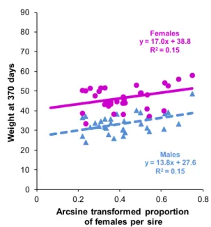
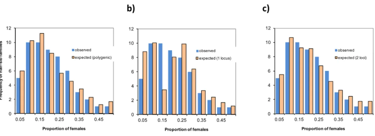
The third paper (section 2.4) describes the between families variation in sex ratio and its co-variation with body weight, and tests several hypotheses about the underlying genetic determinism of sex ratio. There is no genotype by environment component in this paper, as sex was fully determined at tagging, and was therefore not likely to be influenced by the different ongrowing conditions. It is titled "A polygenic hypothesis for sex determination in the European sea bass" by Marc Vandeputte, Mathilde Dupont-Nivet, Hervé Chavanne and Béatrice Chatain and was published in 2007 in Genetics (volume 176: 1049-1057). Complementary (unpublished) information about the threshold model for sex determination and some genetic and environmental correlations between size and sex ratio at different ages is added at the end of section 2.4.
Chapter 3
is about the response to domestication and selection for increased body size, in terms of growth and sex ratio. The related experiments were done in the frame of the European project Competus, funded by the farms Ardag (Israel), Ecloserie Marine de Gravelines (France), Les Poissons du Soleil (France), Tinamenor SA (Spain), Viveiro Vilanova (Portugal) and the European Union (COOP-CT-2005-017633).Direct selection response in terms of growth is studied in section 3.1, where we compare the offspring of wild founders, domesticated (first generation hatchery bred) and selected (2 populations, one mass selected for growth in Ifremer and the other in Panittica Pugliese, with a different protocol) sea bass populations. The paper, "Response to domestication and selection for growth in the European sea bass (Dicentrarchus labrax) in separate and mixed tanks" by Marc Vandeputte, Mathilde Dupont-Nivet, Pierrick Haffray, Hervé Chavanne, Silvia Cenadelli, Katia Parati, Marie-Odile Vidal, Alain Vergnet and Béatrice Chatain was published in 2009 in Aquaculture (volume 286: 20-27).
Correlated responses in terms of sex ratio to domestication and selective breeding for body size is the subject of section 3.2., where we first present evidence on the sex ratio in natural populations of sea bass. As pointed out before, this essential information was lacking in the numerous studies about the causes of sex ratio variations in farmed sea bass, and we felt it was a necessary starting point to