Multiple-Outcome Proof Number Search
Abdallah Saffidine
1and Tristan Cazenave
1Abstract. We present Multiple-Outcome Proof Number Search (MOPNS), a Proof Number based algorithm able to prove positions in games with multiple outcomes.MOPNSis a direct generalization of Proof Number Search (PNS) in the sense that both behave exactly the same way in games with two outcomes. However,MOPNS tar-gets a wider class of games. When a game features more than two outcomes,PNScan be used multiple times with different objectives to finally deduce the value of a position. On the contrary,MOPNSis called only once to produce the same information. We present exper-imental results on solving various positions of the gamesCONNECT FOURandWOODPUSHshowing that in most problems, the total num-ber of node creations ofMOPNSis lower than the cumulative number of node creations ofPNS, even in the best case wherePNSdoes not need to perform a binary search.
1
INTRODUCTION
Proof Number Search (PNS) [4] is a best first search algorithm that enables to dynamically focus the search on the parts of the search tree that seem to be easier to solve. WhilePNSis primarily applicable to games with two outcomes, win and loss, it can also solve games with more than two outcomes using a binary search and thresholds on the outcomes.PNSbased algorithms have been successfully used in many games and especially as a solver for difficult games such as
CHECKERS[17],SHOGI[19], andGO[7].
In this paper, we propose a new effort number based algorithm that enables to solve games with multiple outcomes. The principle guiding our algorithm is to use the same tree for all possible out-comes. When using a dichotomicPNS, the search trees are indepen-dent of each other and the same subtrees are expanded again. We avoid this re-expansion sharing the common nodes. Moreover we can safely prune some nodes using considerations on bounds as in Score Bounded Monte Carlo Tree Search (MCTS) [6].
There has been a lot of developments of the originalPNS algo-rithm [4]. An important problem related to PNS is memory con-sumption as the tree has to be kept in memory. In order to alleviate this problem, V. Allis proposed PN2[3]. It consists in using a sec-ondaryPNSat the leaves of the principalPNS. It allows to have much more information than the originalPNSfor equivalent memory, but costs more computation time. PN2 has recently been used to solve
FANORONA[15].
The main alternative to PN2 is the Depth-First Proof Number Search (DFPN) algorithm [11].DFPNis a depth-first variant ofPNS
based on the iterative deepening idea.DFPNwill explore the game tree in the same order asPNSwith a lower memory footprint but at the cost of re-expanding some nodes.
1 LAMSADE, Université Paris-Dauphine, France.
[email protected], [email protected]
Conspiracy numbers search [8, 16] also deals with a range of pos-sible evaluations at the leaves of the search tree. However, the algo-rithm works with a heuristic evaluation function whereas Multiple-Outcome Proof Number Search (MOPNS) has no evaluation function and only scores solved positions. Moreover the development of the tree is not the same forMOPNSand for Conspiracy numbers search sinceMOPNS tries to prove the outcome that costs the less effort whereas Conspiracy numbers search tries to eliminate unlikely val-ues of the evaluation function.
The IterativePNSalgorithm [9] also deals with multiple outcomes but uses the usual proof and disproof numbers as well as a value for each node and a cache. The main difference between Iterative
PNSand the proposedMOPNS, is that IterativePNStries to find the value of the game by eliminating outcomes step by step. On the other hand,MOPNScan dynamically focus on newly promising values even if previously promising values have not been completly outruled yet. The next section gives some definitions that will be used in the remainder of the paper. The third section detailsPNS. The fourth sec-tion explainsMOPNS. The fifth section gives experimental results for the gamesCONNECT FOURandWOODPUSH.
2
DEFINITIONS
We consider a two player game. The players are named Max and Min. O = {o1, . . . , om} denotes the possible outcomes of the game.
We assume that the outcomes are linearly ordered with the following preference relation for Max: o1 <Max · · · <Max om, we further
as-sume that the game is zero-sum and derive a preference relation for Min: om <Min · · · <Min o1. In the following, we will always stand
in the point of view from Max and use oi < oj(resp. oi≤ oj) as a
shorthand for oi<Maxoj(resp. ¬oi<Minoj).
We assume the game is finite, acyclic, sequential and determinis-tic. Each position n is either terminal or internal and some player is to move. When a position n is internal and player p is to play, we call children of n (noted chil(n)) the positions that can be reached by a move of p. Using backward induction, we can therefore associate to each position n a so-called minimax value, noted real(n) ∈ O.
Solving a position consists in obtaining its minimax value. It is possible to compute directly the minimax value of a given position by building the whole subsequent game tree and using straightforwardly the definition of minimax values. This naive procedure, however, is resource intensive and more practical methods can be sought. Indeed, not every part of the subsequent game tree is needed to compute the minimax value of a position. For instance, if we know that Max is to play in a position n and one child has the best value possible, then real(n) does not depend on the value of the other children and they need not be calculated.
As the current game tree is not necessarily completely expanded, the following classification of nodes arises. Internal nodes
corre-spond to internal positions and have their children in the tree. Ter-minal nodescorrespond to terminal positions and have no children. Non-terminal leaf nodes (leaves for short) correspond to internal po-sitions and do not have their children in the tree.
We call effort numbers heuristic numbers which try to quantify the amount of information needed to prove some fact about the minimax value of a position. The higher the number, the larger the missing piece of information needed to prove the result. When an effort num-ber reaches 0, then the corresponding fact has been proved to be true, while if it reaches ∞ then the corresponding fact has been proved to be false.
3
PROOF NUMBER SEARCH
PNSis an algorithm that can solve positions without exploring the whole game tree. It is essentially designed for games with two out-comes O = {Lose, Win}. In the context ofPNS, proving that the minimax value of a node is Win is called proving the node, while proving that it is Lose is called disproving the node.
3.1
Determination of the effort
PNSis a best first search algorithm which tries to minimize the effort needed to solve the root position. Two effort numbers are associated to each node in the tree, the proof number (PN) represents an esti-mation of the remaining effort needed to prove the node, while the disproof number (DN) represents an estimation of the remaining ef-fort needed to disprove the node. When a node n has been proved, we have PN(n) = 0 and DN(n) = ∞, when n has been disproved, PN(n) = ∞ and DN(n) = 0.
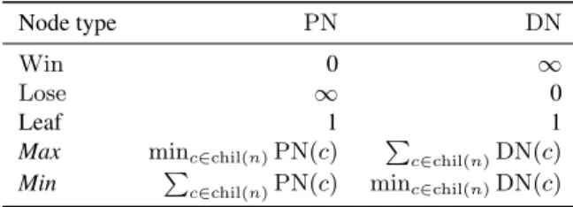
The effort needed to solve a node in the tree is determined in dif-ferent ways depending on its type. They are summarized in Figure 1. The Win and Lose rows designate terminal nodes, in which case the node is already solved. The Leaf row designates a leaf node. Such a node has not been expanded yet, and the proof and disproof num-bers are initially set to 1, although more elaborate initializations exist (see Section 4.6). The Max (resp. Min) row designates internal nodes where Max (resp. Min) is to play. For such nodes, the numbers are deduced from the effort numbers of the children nodes.
Node type PN DN
Win 0 ∞
Lose ∞ 0
Leaf 1 1
Max minc∈chil(n)PN(c)
P
c∈chil(n)DN(c)
Min P
c∈chil(n)PN(c) minc∈chil(n)DN(c)
Figure 1: Determination of effort numbers forPNS
3.2
Descent and expansion of the tree
If the root node is not solved, then more information needs to be added to the tree. Therefore a (non-terminal) leaf needs to be ex-panded. To select it, the tree is recursively descended selecting at each Max node the child minimizing the proof number and at each Minnode the child minimizing the disproof number.
Once the node to be expanded, n, is reached, each of its children are added to the tree. Thus the status of n changes from leaf to in-ternal node and PN(n) and DN(n) have to be updated. This update
may in turn lead to an update of the proof and disproof numbers of its ancestors.
After the proof and disproof numbers in the tree are updated to be consistent with formulae from Figure 1, another most proving leaf can be expanded. The process continues iteratively with a descent of the tree, its expansion and the consecutive update until the root node is solved.
3.3
Multi-outcome games
Many interesting games have more than two outcomes, for instance
CHESS,DRAUGHTSandCONNECT FOURhave three outcomes: O = {Win, Draw, Lose}. We describe the game ofWOODPUSHin the fifth section. A game ofWOODPUSHof size S has 2 × S × (S + 1) possible outcomes. For many games, it is not only interesting to know who is the winner but also what is the exact score of the game.
If there are more than two possible outcomes, the minimax value of the starting position can still be found withPNSby using a di-chotomic search [4]. This didi-chotomic search is actually usingPNSon transformed games. The transformed games have exactly the same rules and game tree as the original one but have binary outcomes. If there are m different outcomes, then the dichotomic search will make about lg(m) calls toPNS.
If the minimax value is already known, e.g., from expert knowl-edge, but needs to be proved, then two calls toPNSare necessary and sufficient.
4
MULTIPLE-OUTCOME PROOF NUMBER
SEARCH
MOPNSaims at applying the ideas fromPNSto multi-outcome games. However, contrary to dichotomicPNSand iterativePNS,MOPNS dy-namically adapts the search depending on the outcomes and searches the same tree for all the possible outcomes.
MOPNSshares many similarities withPNS. A game tree is kept in memory and it is extended through cycles of descent, expansion and updates.MOPNSalso makes use of effort numbers.
In PNS, two effort numbers are associated with every node, whereas inMOPNS, if there are m outcomes, then 2m effort num-bers are associated with every node. InPNS, only completely solved subtrees can be pruned, while pruning plays a more important role in
MOPNSand can be compared to alpha-beta pruning.
4.1
Effort Numbers
MOPNSalso uses the concept of effort numbers but different num-bers are used here in order to account for the multiple outcomes. Let n be a node in the game tree, and o ∈ O an outcome. The greater number, G(n, o), is an estimation of the number of node expansions required to prove that the value of n is greater than or equal to o (from the point of view of Max), while conversely the smaller number, S(n, o), is an estimation of the number of node ex-pansions required to prove that the value of n is smaller than or equal to o. If G(n, o) = S(n, o) = 0 then n is solved and its value is o: real(n) = o.
Figure 2 features an example of effort numbers for a three out-comes game. The effort numbers show that in the position under consideration Max can force a draw and it seems unlikely that at that point the Max can force a win.2
2S(n, Win) 6= 0 means that it was not assumed that the game is finite and
Outcome G S
Win 500 3
Draw 0 10
Lose 0 ∞
Figure 2: Example of effort numbers for a 3 outcome game
4.2
Determination of the effort
The effort numbers of internal nodes are obtained in a very similar fashion toPNS, G is analogous to PN and S is analogous to DN. Ev-ery effort number of a leaf is initialized at 1, while the effort numbers of an internal node are calculated with the sum and min formulae as shown in Figure 3a.
If n is a terminal node and its value is real(n), then the effort numbers are associated as shown in Figure 3b. We have for all o ≤ real(n), G(n, o) = 0 and for all o ≥ real(n), S(n, o) = 0.
Node type G(n, o) S(n, o)
Leaf 1 1
Max minc∈chil(n)G(c, o) Pc∈chil(n)S(c, o)
Min P
c∈chil(n)G(c, o) minc∈chil(n)S(c, o)
(a) Internal node
Outcome G S om ∞ 0 . . . ∞ 0 real(n) 0 0 . . . 0 ∞ o1 0 ∞ (b) Terminal node
Figure 3: Determination of effort numbers forMOPNS
4.3
Properties
G(n, o) = 0 (resp. S(n, o) = 0) means that the value of n has been proved to be greater than (resp. smaller) or equal to o, i.e., Max (resp. Min) can force the outcome to be at least o (resp. at most o). Conversely G(n, o) = ∞ means that it is impossible to prove that the value of n is greater than or equal to o, i.e., Max cannot force the outcome to be greater than or equal to o.
As can be observed in Figure 2, the effort numbers are mono-tonic in the outcomes. If oi ≤ ojthen G(n, oi) ≤ G(n, oj) and
S(n, oi) ≥ S(n, oj). Intuitively, this property states that the better an
outcome is, the harder it will be to obtain it or to obtain better. 0 and ∞ are permanent values since when an effort number reached 0 or ∞, its value will not change as the tree grows and more information is available. Several properties link the permanent values of a given node. The proofs are straightforward recursions from the leaves and are omitted for lack of space. Care must only be taken that the initialization of leaves satisfies the property which is the case for all the initializations discussed here.
Proposition 1. If G(n, o) = 0 then for all o0 < o, S(n, o0) = ∞ and similarly ifS(n, o) = 0 then for all o0> o, G(n, o0) = ∞. Proposition 2. If G(n, o) = ∞ then S(n, o) = 0 and similarly if S(n, o) = ∞ then G(n, o) = 0.
4.4
Descent policy
We call attracting outcome of a node n, the outcome o∗(n) that has not been proved to be achievable by the player on turn and minimiz-ing the sum of the correspondminimiz-ing effort numbers. We have for Max nodes o∗(n) = arg mino,G(n,o)>0(G(n, o)+S(n, o)). Similarly, we
have for Min nodes o∗(n) = arg mino,S(n,o)>0(G(n, o) + S(n, o)). As a consequence of the existence of a minimax value for each po-sition, for all node n, there always exists at least one outcome o, such that G(n, o) 6= ∞ and S(n, o) 6= ∞. Hence, G(n, o∗(n)) + S(n, o∗(n)) 6= ∞.
We call distracting outcome of a Max (resp. Min) node n the outcome just below (resp. above) its attracting outcome, we note it o0(n). When the attracting outcome of a Max (resp. Min) node is the worst (resp. best) outcome in the game, we set the distracting outcome to be equal to the most likely outcome. That is, if n is a Maxnode with o∗(n) = ok, then o0(n) = omax(k−1,1)and if n is
a Min node, then o0(n) = omin(k+1,m). As the name indicates, the
distracting outcome of a node is the one towards which it would be simplest for the opponent to deviate if he or she wanted to disprove the attracting outcome.
Consider Figure 2, if these effort numbers were associated to a Maxnode, then the attracting outcome would be Win and the dis-tracting outcome would be Draw, while if they were associated to a Minnode then the attracting outcome would be Draw and the dis-tracting outcome would be Win.
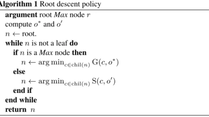
From now on, unless we specify otherwise, we will only consider the attracting and distracting outcomes of the root node r of the tree and note o∗ = o∗(r), o0 = o0(r). We assume Max is at turn in the root node. We can now define the root descent policy that specify how the leaf to be expanded is selected (see Algorithm 1). We first estimate which outcome is attracting at the root node, then we try to prove this value at Max nodes and to disprove it at Min nodes. Algorithm 1 Root descent policy
argument root Max node r compute o∗and o0 n ← root.
while n is not a leaf do if n is a Max node then
n ← arg minc∈chil(n)G(c, o ∗
) else
n ← arg minc∈chil(n)S(c, o 0
) end if
end while return n
Proposition 3. For finite two outcome games,MOPNSandPNS de-velop the same tree.
Proof. If we know the game is finite, the Max is sure to obtain at least the worst outcome so we can initialize the greater number for the worst outcome to 0, we can also initialize the smaller number for the best outcome to 0. If there are two outcomes only, O = {Lose, Win}, then we have the following relation between effort numbers inPNSandMOPNS: G(n, Win) = PN(n), S(n, Lose) = DN(n). If the game is finite with two outcomes, then the attract-ing outcome of the root is Win and the distractattract-ing outcome is Lose. Hence,MOPNSandPNSbehave in the same manner.
4.5
Pruning
We define the pessimistic and optimistic bounds for a node n as pess(n) = arg maxo(G(n, o) = 0) and opti(n) =
arg mino(S(n, o) = 0). The following inequality gives their name to the bounds pess(n) ≤ real(n) ≤ opti(n), pess(n) (resp. opti(n)) is the worst value possible (resp. the best value possible) for n con-sistent with the current information in the tree. For any node n, n is solved as soon as pess(n) = opti(n). Although the definition is dif-ferent, these bounds coincide with those described in Score Bounded Monte Carlo Tree Search [6].
We also define relevancy bounds that are similar to alpha and beta bounds in the classic Alpha-Beta algorithm [13]. For a node n, the lowerrelevancy bound is noted α(n) and the upper relevancy bound is noted β(n). These bounds are calculated using the optimistic and pessimistic bounds as follows. If n is the root of the tree, then α(n) = pess(n) and β(n) = opti(n). Otherwise, we use the rele-vancy bounds of the father node of n: if n ∈ chil(f ), we set α(n) = maxMax(α(f ), pess(n)) and β(n) = minMax(β(f ), opti(n)).
The relevancy bounds of a node n take their name from the fact that if real(n) ≤ α(n) or if real(n) ≥ β(n), then having more information about real(n) will not contribute to solving the root of the tree. Therefore they enable safe pruning.
Proposition 4. For each node n, if we have β(n) ≤ α(n) then the the subtree ofn need not be explored any further.
Subtrees starting at a pruned node can be completely removed from the main memory as they will not be used anymore in the proof. This improvement is crucial as lack of memory is one of the main bottleneck ofPNSandMOPNS.
We now show that pruning does not interfere with the root descent policy in the sense that it will not affect the number of descents per-formed before the root is solved. For this purpose, we prove that the root descent policy does not lead to a node which can be pruned. Proposition 5. If r is not solved, then for all nodes n traversed by the root descent policy,α(n) < o∗≤ β(n).
Proof. We first prove the inequality for the root node. If the root po-sition r is not solved, then by definition of the attractive outcome, o∗ > pess(r) = α(r). Using Proposition 1, we know that all out-comes better than the optimistic bound cannot be achieved: ∀o > opti(r) = β(r), G(o, r) = ∞. Since G(r, o∗) + S(r, o∗) 6= ∞, then α(r) < o∗≤ β(r).
For the induction step, suppose n is a Max node that satisfies the inequality. We need to show that c = arg minc∈chil(n)G(c, o
∗
) also satisfies the inequality. Recall that the pessimistic bounds of n and c satisfy the following order: pess(c) ≤ pess(n) and ob-tain the first part of the inequality α(c) = α(n) < o∗. From the induction hypothesis, o∗ ≤ β(n) ≤ opti(n), so from Proposi-tion 1 G(n, o∗) 6= ∞, moreover, the selection process ensures that G(c, o∗) = G(n, o∗) 6= ∞, therefore G(c, o∗) 6= ∞ which using Proposition 2 leads to o∗≤ opti(c). Thus, o∗≤ β(c). The induction step when n is a Min node is similar and is omitted.
4.6
Applicability of classical improvements
Many improvements of PNSare directly applicable toMOPNS. For instance, the current-node enhancement presented in [3] takes ad-vantage of the fact that many consecutive descents occur in the same subtree. This optimization allow to obtain a notable speed-up and can be straightforwardly applied toMOPNS.
It is possible to initialize leaves in a more elaborate way than pre-sented in Figure 3a. Most initializations available toPNScan be used withMOPNS, for instance the mobility initialization [20] in a Max node n consists in setting the initial smaller number to the number of legal moves: G(n, o) = 1, S(n, o) = | chil(n)|. In a Min node, we would have G(n, o) = | chil(n)|, S(n, o) = 1.
A generalization of PN2is also straightforward. If n is a new leaf and d descents have been performed in the main tree, then we run a nestedMOPNSindependent from the main search starting with n as root. After at most d descents are performed, the nested search is stopped and the effort numbers of the root are used as initializa-tion numbers for n in the main search. We can safely propagate the interest bounds to the nested search to obtain even more pruning.
Similarly, a transformation ofMOPNSinto a depth-first search is possible as well, adapting the idea of Nagai [11]. Just as in DFPN, only two threshold numbers would be needed during the descent, one threshold would correspond to the greater number for the current attractive outome at the root and one threshold would correspond to the smaller number for the distractive outcome.
Finally, given thatMOPNSis very close in spirit toPNS, a care-ful implementer should not face many problems adapting the various improvements that make DFPN such a successful technique in prac-tice. Let us mention in particular Nagai’s garbage collection tech-nique [11], Kishimoto and Müller’s solution to the Graph History Interaction problem [7], and Pawlewicz and Lew’s 1 + ε trick [12].
5
EXPERIMENTAL RESULTS
To assess the validity of our approach, we implemented a prototype ofMOPNSand tested it on two games with multiple outcomes, namely
CONNECT FOUR and WOODPUSH. Our prototype does not detect transposition and is implemented via the best first search approach described earlier. As such, we compare it to the original best-first variation ofPNS, also without transposition detection. Note that the domain ofCONNECT FOURandWOODPUSHare acyclic, so we do not need to use the advanced techniques presented by Kishimoto and Müller to address the Graph History Interaction problem [7]. Addi-tionally, the positions that constitute our testbed were easy enough that they could be solved by search trees of at most a few million nodes. Thus, the individual search trees forPNSas well asMOPNS
could fit in memory without ever pruning potentially useful nodes. In our implementation, the two algorithms share a generic code for the best first search module and only differ on the initialization, the update, and the selection procedures. The experimental results were obtained running OCaml 3.11.2 under Ubuntu on a laptop with Intel T3400 CPU at 2.2 GHz and 1.8 GiB ofmemory.
For each test position and each possible outcome, we performed one run of the PNS algorithm and recorded the time the number of node creation it needed. We then discarded all but the two runs needed to prove the final result. For instance, if a position inWOOD
-PUSHadmitted non-zero integer scores between −5 and +5 and its perfect play score was 2, we would runPNSten times, and finally out-put the measurements for the run proving that the score is greater or equal to 2 and the measurements for the run disproving that the score is greater or equal to 3. This policy is beneficial toPNScompared to doing a binary search for the outcome.
To compareMOPNStoPNSon a wide range of positions, we created the list of all positions reached after a given number of moves from the starting position of a given size. These positions range from being vastly favourable to Min to vastly favourable to Max, and from triv-ial (solved in a few milliseconds) to more involved (each run being
around two to three minutes).
5.1
CONNECT FOURCONNECT FOURis a commercial two-player game where players drop a red or a yellow piece on a 7 × 6 grid. The first player to align four pieces either horizontally, vertically or diagonally wins the game. The game ends in a draw if the board is filled and neither player has an alignment. The game was solved by James D. Allen and Victor Allis in 1988 [2].
Table 1 presents aggregate data over our experiments on size 4 × 5 and 5×5. In both cases, we used the positions occuring after 4 moves. In the first case, 16 positions among the 256 positions tested were a first player win, 222 were a draw while 18 were a first player loss. In the second list of positions, there were 334 wins, 267 draws, and 24 losses.
Table 1: Cumulated time and number of node creation for theMOPNS
andPNSalgorithms in the game ofCONNECT FOUR. For both algo-rithm, Lowest time indicates the number of positions that were soved faster by this algorithm, while Lowest node creations indicates the number of positions which needed fewer node creations.
MOPNS PNS
Size 4 × 5, 256 positions after 4 moves
Total time (seconds) 99 85 Total node creations 16,947,536 20,175,238
Lowest time 21 235
Lowest node creations 227 13 Size 5 × 5,
625 positions after 4 moves
Total time (seconds) 11,230 9055 Total node creations 1,557,490,694 1,757,370,222
Lowest time 55 570
Lowest node creations 406 140
Figure 4 plots the number of node creations needed to solve each of the 256 4×5 positions. We can see that for a majority of positions,
MOPNSneeded fewer node creations thanPNS. There are 16 positions that needed the same number of node creations by both algorithm and these positions are exactly the positions that are first player wins.
104 105 104 105 Node creations PNSnode creations MOPNS PNS
Figure 4: Comparison of the number of node creations forMOPNSand
PNSfor solving 256CONNECT FOURpositions on size 4 × 5.
5.2
WOODPUSHThe game ofWOODPUSHis a recent game invented by combinatorial game theorists to analyze a game that involves forbidden repetition of
the same position [1, 5]. A starting position consists of some pieces for the left player and some for the right player put on an array of pre-defined length as shown in Figure 5. A Left move consists in sliding one of the left pieces to the right. If some pieces are on the way of the sliding piece, they are jumped over. When a piece has an opponent piece behind it, it can move backward and push all the pieces behind, provided it does not repeat the previous position. The game is won when the opponent has no more pieces on the board. The score of a game is the number of moves that the winner can play before the board is completely empty.
#
#
Figure 5:WOODPUSHstarting position on size (10, 2) The experimental protocol forWOODPUSHwas similar to that of
CONNECT FOUR. The first list of problems corresponds to positions occuring after 4 moves on a board of length 8 with 3 pieces for each player. The second list of problems corresponds to positions occuring after 8 moves on a board of length 13 with 2 pieces for each player. Table 2 presents aggregates data for the solving time and the num-ber of node creations, while Figure 6 presents the numnum-ber of node creations for each problem in the second list.
Table 2: Cumulated time and number of node creation for theMOPNS
andPNSalgorithms in the game ofWOODPUSH.
MOPNS PNS
Size (8, 3), 99 positions after 4 moves
Total time (seconds) 718 702 Total node creations 31,328,178 34,869,213
Lowest time 25 74
Lowest node creations 76 23 Size (13, 2),
256 positions after 8 moves
Total time (seconds) 4796 4573 Total node creations 155,756,022 174,285,199
Lowest time 98 158
Lowest node creations 205 51
105 106 105 106 Node creations PNSnode creations MOPNS PNS
Figure 6: Comparison of the number of node creations forMOPNSand
PNSfor solving 256WOODPUSHpositions on size (13, 2).
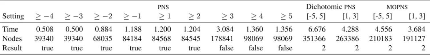
InWOODPUSH(8, 3), it is possible to create final positions with scores ranging from −18 to 18 but these positions might not be ac-cessible from the start position. Indeed, in our experiments, no final position with a score below −5 or over 5 was ever reached. How-ever, while the scores remained between −5 and 5, the exact range varied depending on the problem. While doing a binary search for the
Table 3: Detailed results for the 86th
WOODPUSHproblem on size (8, 3).
PNS DichotomicPNS MOPNS
Setting ≥ −4 ≥ −3 ≥ −2 ≥ −1 ≥ 1 ≥ 2 ≥ 3 ≥ 4 ≥ 5 [-5, 5] [1, 3] [-5, 5] [1, 3] Time 0.508 0.500 0.884 1.188 1.200 1.204 3.084 1.360 1.356 6.676 4.288 4.556 3.684 Nodes 39340 39340 68035 84184 84568 84545 178841 98069 98069 351366 263386 210183 191127 Result true true true true true true false false false 2 2 2 2 outcome is the natural generic process for solving a multi-outcome
game withPNS, we decided to compareMOPNSto the ideal case for
PNSwhich only involves two runs per position. On the other hand, we only assumed forMOPNSthat the outcome was in [−5, 5]. Therefore, the results presented in Table 2 and Figure 6 significantly favourPNS. Table 3 details the results for the position presented in Figure 7. ThePNStree did not access any position with a score lower or equal to −4 nor any position with a score greater or equal to 5.
#
#
#
Figure 7: 86thWOODPUSHproblem on size (8, 3).
6
CONCLUSION AND DISCUSSION
We have presented a generalized Proof Number algorithm that solves games with multiple outcomes in one run. Running PNSmultiple times to prove an outcome develops the same nodes multiple times while inMOPNSthese nodes are developed only once. MOPNShas been formally proved equivalent toPNSin two-outcome games and we have shown how safe pruning could be performed in multiple out-come games. For smallCONNECT FOURandWOODPUSHboards, in most casesMOPNSsolves the games with fewer node creations than
PNSeven if it already knows the optimal outcome of the game and no binary search is needed.
We have assumed in this article that the game structure was a tree. In most practical cases it actually is a Directed Acyclic Graph (DAG) and in some cases the graph contains cycles.3The theoretical results presented in this article still hold in theDAGcase, provided the def-inition of the relevancy bounds is adapted to reflect the fact that a node may have multiple parents and some of them might not yet be in the tree. The double count problem ofPNSwill also affectMOPNS
inDAGs, but it is possible to take advantage of previous work on the handling of transpositions inPNS[18, 10]. Similarly, the problems encountered byMOPNSin cyclic graphs are similar to that ofPNSand
DFPNin cyclic graphs. Fortunately, it should be straightforward to adapt Kishimoto and Müller’s ideas [7] fromDFPNto a depth-first version ofMOPNS.
In future work, we plan on trying to adapt the PN2paralellization scheme suggested by Saffidine et al. [14] to games with multiple out-comes viaMOPNS. We would also like to study a depth-first version ofMOPNSthat can be obtained via Nagai’s transformation [11].
Finally, studying howMOPNScan be extended to deal with prob-lems where the outcome space is not known beforehand or is con-tinuous in order to develop an effort number algorithm for non-deterministic two-player games is definitely an attractive research agenda.
3For instance, the original rules forCHESSresult in aDAGbecause of the
50-moves rule, but this rule is usually abstracted away, resulting in a cyclic structure.
REFERENCES
[1] Michael H. Albert, Richard J. Nowakowski, and David Wolfe, Lessons in play: an introduction to combinatorial game theory, AK Peters Ltd, 2007.
[2] Louis Victor Allis, A Knowledge-based Approach of Connect-Four The Game is Solved: White Wins, Masters thesis, Vrije Universitat Amster-dam, AmsterAmster-dam, The Netherlands, October 1988.
[3] Louis Victor Allis, Searching for Solutions in Games an Artificial Intel-ligence, Phd thesis, Vrije Universitat Amsterdam, Department of Com-puter Science, Rijksuniversiteit Limburg, 1994.
[4] Louis Victor Allis, M. van der Meulen, and H. Jaap van den Herik, ‘Proof-Number Search’, Artificial Intelligence, 66(1), 91–124, (1994). [5] Tristan Cazenave and Richard J. Nowakowski, ‘Retrograde analysis of
woodpush’, in Games of no chance 4, to appear.
[6] Tristan Cazenave and Abdallah Saffidine, ‘Score bounded Monte-Carlo tree search’, in Computers and Games, eds., H. van den Herik, Hiroyuki Iida, and Aske Plaat, volume 6515 of Lecture Notes in Computer Sci-ence, 93–104, Springer-Verlag, Berlin / Heidelberg, (2011).
[7] Akihiro Kishimoto and Martin Müller, ‘A solution to the GHI prob-lem for depth-first proof-number search’, Information Sciences, 175(4), 296–314, (2005).
[8] David A. McAllester, ‘Conspiracy numbers for min-max search’, Arti-ficial Intelligence, 35(3), 287–310, (1988).
[9] Carsten Moldenhauer, Game tree search algorithms for the game of cops and robber, Master’s thesis, University of Alberta, September 2009.
[10] Martin Müller, ‘Proof-set search’, in Computers and Games 2002, Lec-ture Notes in Computer Science, 88–107, Springer, (2003).
[11] Ayumu Nagai, Df-pn algorithm for searching AND/OR trees and its applications, Ph.D. dissertation, University of Tokyo, December 2001. [12] Jakub Pawlewicz and Łukacz Lew, ‘Improving depth-first PN-search: 1+ε trick’, in Proceedings of the 5th international conference on Com-puters and games, pp. 160–171. Springer-Verlag, (2006).
[13] Stuart J. Russell and Peter Norvig, Artificial Intelligence — A Modern Approach, Pearson Education, third edn., 2010.
[14] Abdallah Saffidine, Nicolas Jouandeau, and Tristan Cazenave, ‘Solving Breakthough with race patterns and Job-Level Proof Number Search’, in Advances in Computer Games, Springer-Verlag, Berlin / Heidelberg, (2011).
[15] Maarten P.D. Schadd, Mark H.M. Winands, Jos W.H.M. Uiterwijk, H. Jaap van den Herik, and M.H.J. Bergsma, ‘Best Play in Fanorona leads to Draw’, New Mathematics and Natural Computation, 4(3), 369– 387, (2008).
[16] Jonathan Schaeffer, ‘Conspiracy numbers’, Artificial Intelligence, 43(1), 67–84, (1990).
[17] Jonathan Schaeffer, Neil Burch, Yngvi Björnsson, Akihiro Kishimoto, Martin Müller, Robert Lake, Paul Lu, and Steve Sutphen, ‘Checkers is solved’, Science, 317(5844), 1518, (2007).
[18] Martin Schijf, L. Victor Allis, and Jos W.H.M. Uiterwijk, ‘Proof-number search and transpositions’, ICCA Journal, 17(2), 63–74, (1994).
[19] Masahiro Seo, Hiroyuki Iida, and Jos W.H.M. Uiterwijk, ‘The PN*-search algorithm: Application to tsume-shogi’, Artificial Intelligence, 129(1-2), 253–277, (2001).
[20] H. Jaap van den Herik and Mark Winands, ‘Proof-Number Search and its variants’, Oppositional Concepts in Computational Intelligence, 91– 118, (2008).