Ardia: Corresponding author. Département de finance, assurance et immobilier, Université Laval, Québec, Canada; and CIRPÉE
david.ardia@fsa.ulaval.ca
Gatarek: Erasmus School of Economics, Erasmus University Rotterdam, Rotterdam, The Netherlands; Tinbergen Institute, The Netherlands
gatarek@tlen.pl
Hoogerheide: Department of Econometrics, Vrije Universiteit Amsterdam, The Netherlands; Tinbergen Institute, The Netherlands
l.f.hoogerheide@vu.nl
We are grateful to Kris Boudt for numerous comments. Any remaining errors or shortcomings are the authors’ responsibility.
Cahier de recherche/Working Paper 14-13
A New Bootstrap Test for the Validity of a Set of Marginal Models for
Multiple Dependent Time Series: an Application to Risk Analysis
David Ardia Lukasz Gatarek
Lennart F. Hoogerheide
Abstract:
A novel simulation-based methodology is proposed to test the validity of a set of marginal time series models, where the dependence structure between the time series is
taken ‘directly’ from the observed data. The procedure is useful when one wants to
summarize the test results for several time series in one joint test statistic and p-value. The proposed test method can have higher power than a test for a univariate time series, especially for short time series. Therefore our test for multiple time series is particularly useful if one wants to assess Value-at-Risk (or Expected Shortfall) predictions over a small time frame (e.g., a crisis period). We apply our method to test GARCH model specifications for a large panel data set of stock returns.
Keywords: Bootstrap test, GARCH, Marginal models, Multiple time series, Value-at-Risk
1. Introduction
In several situations one desires to evaluate the validity of a set of models for dependent uni-variate time series. Therefore, a test of the joint validity is desirable. In this paper, a novel simulation-based methodology is proposed to test the validity of a set of marginal time series models, where the dependence structure between the time series is taken ‘directly’ from the ob-served data. Since the dependence structure is not tested, the procedure is useful in the following situations. First, the case where one has specified the dependence structure, but where one specif-ically desires to test only the marginal models; for example, as an additional tool for assessing the univariate specifications in a copula model, without testing the validity of the particular copula choice. That is, a separate goodness-of-fit test can be applied for the copula specification. Second, the case where no dependence structure is specified; for example, when one wants to summarize the test results of a proposed model or method for several time series in one joint test statistic and p-value.
We apply our method to test GARCH model specifications for a large panel data set of stock returns; from a practical viewpoint, it is desirable to have a single model for many time series. The proposed test method can have higher power than a test for a univariate time series, especially for short time series. The reference test by Christoffersen (1998) for testing the Value-at-Risk performance may require a large number of observations, in order to have a reasonable power. Therefore our test for multiple time series is particularly useful if one wants to assess Value-at-Risk (or Expected Shortfall) predictions over small time frames such as crisis periods. In particular, we test a range of GARCH models for left-tail density and Value-at-Risk predictions for the universe of S&P 500 equities. We use the new methodology to discuss the application of the models over the whole universe and for subsets of the universe (e.g., sizes or sectors). Also, we make use of the cross-sectional power of the approach to test the models over sub-windows, in particular a crisis period.
A well-known alternative is the Bonferroni correction method, where in a situation of multiple testing the significance level per test is computed as the the total significance level (or family-wise error rate (FWER)) divided by the number of tests. An extension is the Holm-Bonferroni method (Holm, 1979). However, for the null hypothesis that all marginal models are correct this Holm-Bonferroni method reduces to the original Holm-Bonferroni correction. These Holm-Bonferroni correction methods may lead to very low power, especially in cases of large numbers of tests. Furthermore, the Bonferroni correction only leads to rejection or non-rejection in a conservative setting, without explicitly giving an exactly appropriate p-value. This also implies that in certain situations where one wants to retain, not reject, the null hypothesis, the Bonferroni correction is actually non-conservative. ˇSid´ak (1967) proposed an alternative way to improve the power of the Bonferroni correction method, but this method requires the independence of the multiple tests.
Another alternative method to test for the validity of the marginal models may seem the false discovery rate (FDR) methodology of Storey (2002), in combination with the confidence interval for the percentage of correct marginal models of Barras et al. (2010). One could attempt to test the hypothesis that all marginal models are correct by investigating whether the confidence interval for the percentage of correct marginal models contains the value 100%. However, the false discovery rate methodology assumes independence between the different time series (or a ‘limited’ type of
dependence such as independence between a large enough number of subsets), an assumption that may be substantially violated by e.g. time series of asset returns. Storey and Tibshirani (2003) discuss the FDR under different types of dependence. Under their most general assumptions on the dependence their estimator is (conservatively) biased. Further, they consider DNA data, which arguably have a substantially different dependence structure than e.g. time series in economics and finance.
This article continues as follows. In Section 2 we introduce the bootstrap test and discuss applications. In Section 3 we perform a Monte Carlo study to test the performance of the new methodology, where we consider the size and power for simulated data sets. In Section 4 we apply the new method to GARCH models on several equity universes. In particular, we test the forecasting performance of the models over sub-periods such as crisis periods. In Section 5 we discuss some possible extensions and applications. Section 6 concludes.
2. Bootstrap test procedure and its applications
We consider variables yti (t = 1, . . . , T ; i = 1, . . . , N ), where we have N time series of T
periods. We present the test in the context of financial returns for convenience with the latter applications, where ytiis the ex-post return (or profit/loss) of asset i at time t. However, it can be
applied in any situation where the validity of a set of marginal models is tested: H0 : all ‘marginal models’ are correct,
H1 : at least one ‘marginal model’ is incorrect.
(1) Define the probability integral transform (PIT) or p-scores (Diebold et al., 1998) xtias:
xti . = ˆFt|t−1,i(yti) . = Z yti −∞ ˆ ft|t−1,i(u)du , (2)
with ˆft|t−1,i the ex-ante forecasted return density, and ˆFt|t−1,i the ex-ante forecasted return
cumu-lative density function. Only under a correct model specification, i.e., if both the model and the parameter values are correctly specified, the PITs have uniform distributions that are independent over time. The PITs have this property asymptotically if consistent parameter estimators are used (Rosenblatt, 1952). If an invalid model specification is used, then the PITs will have a non-uniform distribution and/or the PITs will be dependent over time. Therefore, it is natural to investigate the PITs of a model in order to assess the validity of a marginal model. Define the matrix X as the (T × N ) matrix of xti (t = 1, . . . , T ; i = 1, . . . , N ). First, compute for each time series (i.e., for
each column of X) the test statistic, for example the LR statistic in a particular test for the validity of the marginal model. Examples of such LR tests include the test for correct unconditional cover-age, independence, or correct conditional coverage of Christoffersen (1998), the tests for correctly distributed or independent durations between ‘violations’ of the Value-at-Risk of Christoffersen and Pelletier (2004), and the test of Berkowitz (2001) with null hypothesis that zti
.
= Φ−1(xti) has
The joint test statistic for all columns (assets) is now a function (yielding a scalar) of the test statistics over the N columns (assets). If this paper we consider the sum of the N test statistics, but a different function such as the maximum could also be used. This choice obviously affects the power against different violations of H0. For example, if each marginal model suffers from a
minor misspecification, then the sum of the N test statistics seems a reasonable choice. If only one marginal model has a substantial misspecification, whereas the other models are correctly specified, then the maximum of the N test statistics seems a reasonable choice. If the N test statistics are LR statistics, then this sum of N test statistics would be the valid joint LR test statistic (asymptotically having a χ2 distribution under H0) if the columns (assets) would be independent.
However, we do not make this (unrealistic) assumption of independence. To take the dependence between the columns/assets into account, we compute the p-value by simulating the distribution of X under H0.
Step 1 Compute the (T × N ) matrix R of which each column contains the ranking numbers of the corresponding column of X.
Step 2 Simulate X under H0: simulate i.i.d. U (0, 1) distributed elements per column, with
depen-dence between elements per row. First, simulate a (T × 1) vector v containing T i.i.d. draws from the discrete uniform distribution on {1, 2, . . . , T }. Second, define the (1 × N ) vector st(t = 1, 2, . . . , T ) as the vt-th row of R. Third, simulate uti (t = 1, . . . , T ; i = 1, . . . , N )
from a beta distribution Beta(sti, T + 1 − sti). Note that we make use of the result that the
sti-th order statistic of T i.d.d. U (0, 1) distributed variables has a B(sti, T + 1 − sti)
distribu-tion. Also, notice that for N = 1 this is a clumsy way of simulating a (T × 1) column vector of i.i.d. U (0, 1) draws (by first simulating the order statistic from {1, 2, . . . , T } and second simulating from the relevant Beta distribution conditional on the simulated order statistic). Now we have a (T × N ) matrix where each column has i.i.d. U (0, 1) draws, but with de-pendence between the elements per row. The reason is that we simulate rows independently, and that the ranking numbers per row are dependent (if the columns of the original data are dependent). The dependence between the columns is preserved.
Step 3 Repeat simulation of X under H0and compute p-value as the fraction of simulated data sets
for which H0 is not rejected. Typically the test statistic can be computed from the PITs;
otherwise, a time series of the original variable can be computed from the PITs and the model.
The computer code of the above steps is straightforward; see Appendix A for a MATLAB imple-mentation.
We can generate many matrices X from the distribution under H0, compute the test statistic
(i.e., the sum of N test statistics) for each simulated data set, and compute the p-value by com-paring the test statistic for the empirical data set with the test statistics for the simulated data sets under H0.
As mentioned before, for the likelihood ratio (LR) tests, the sum of the LR statistics for the univariate time series provides a natural ‘joint’ test statistic for the set of time series, since this amounts to the LR statistics if the series would be independent. The bootstrap method serves as a way to correct the distribution under the null hypothesis, replacing the no longer valid (asymptotic)
χ2 distribution. However, also other test statistics for univariate time series can be summed to
produce a joint test statistic, e.g., F-statistics or Cram´er-von Mises test statistics.
We preserve the dependence between the time series. That is, we take the dependence structure between the time series from the data. For this purpose, we do not require that the dependence structure is constant over time. In the case of a time-varying dependence structure of a stationary process, for large enough samples the distribution of the dependence structure tends to its uncon-ditional distribution. Our experiments in Section 3 illustrate that our approach also works well, in the sense of a U (0, 1) distributed p-value under the null for the continuously distributed test statistic of Berkowitz (2001), for two DGPs involving time-varying dependence structures – one DGP where the time-varying dependence structure is exogenous (a two-regime Markov switch-ing model) and one DGP where the time-varyswitch-ing dependence structure is endogenous (a dynamic conditional correlation model).
In this paper we will consider the following tests: • Berkowitz (2001): We test whether zti
.
= Φ−1(xti) is standard normal and independent over
time. That is, in the model:
zti− µi = ρi(zt−1,i− µi) + εti, εti∼ i.i.d. N (0, σi2) , (3)
we perform the LR test with null hypothesis that µi = 0, ρi = 1, and σ2i = 1. Under the
null hypothesis the LR statistic follows asymptotically a χ2 distribution with three degrees of freedom but we do not make use of this asymptotic distribution, as we only use our simulation-based approach to determine the p-value. We also consider an extension of this LR test, which was suggested by Christoffersen and Pelletier (2004), with specific focus on the left tail. In that extended version of the test, we only select those xitthat are smaller than
α = 0.05 or α = 0.01, after which we test whether zti
.
= Φ−1(xti/α) is standard normal and
independent over time.
• Christoffersen (1998): We perform the LR test for correct conditional coverage of the 95% and 99% Value-at-Risk, i.e., the 5% and 1% percentile of the predicted return’s distribution. That is, for α = 0.05 and α = 0.01 we perform the LR test with null hypothesis that the binary variables: Iti . = ( 1 if xit < α 0 if xit ≥ α , (4)
are independent and Bernoulli distributed with P{Iti = 1} = α, against the alternative that
the Iti follow a first-order Markov chain. This LR test combines the LR tests for correct
unconditional coverage, P{Iti= 1} = α, and independence between Itiand It−1,i.
3.1. Illustration of correct size
In this section we consider the size and power of our proposed approach. We analyze the finite sample performance of the method via some (necessary limited) simulations. First, we illustrate that our test yields a p-value that is U (0,1) distributed under the null. For this purpose we use the test of Berkowitz (2001), for which the test statistic has a continuous distribution. Note that in the tests of Christoffersen (1998) for correct unconditional coverage, independence and correct conditional coverage statistic, the test statistic has a discrete distribution, which implies that even under the null the distribution of the p-value is not U (0,1).
We consider different DGPs with different dependence structures between the time series. For the marginal distributions we consider the convenient N (0,1) distribution, since the choice of the marginal distribution does not matter in these experiments. The marginal is anyway correct under the null hypothesis, so that the PIT will anyway be U (0, 1) distributed for the marginal models. We consider the following three data generating processes (DGPs):
• Constant correlation model: The data generating process for the (N × 1) vector ytis given
by:
yt ∼ i.i.d. N (0, Σ) (5)
Σ= ρ J + (1 − ρ) I ,. (6)
with J a (N × N ) matrix of ones and I the (N × N ) identity matrix. We set ρ = 0.9. • Two-regime Markov switching correlation model:
yt∼ N (0, Σst) (7)
Σst
.
= ρstJ + (1 − ρst) I , (8)
with {st} a sequence assumed to be a stationary, irreducible, Markov process with discrete
state space {1, 2} and transition matrix P = [P. ij] where Pij
.
= P{st+1 = j | st = i}. We
consider ρ1 = 0.9, ρ2 = 0, P11= 0.9 and P22= 0.9. Note that the time-varying dependence
structure is exogenous here, in the sense that the dependence structure at time t only depends on the dependence structure at time t − 1, and not on yt−1(given the dependence structure
at time t − 1).
• Dynamic conditional correlation model: The data generating process for the (N × 1) vector ytis given by:
yt∼ N (0, Σt) (9)
Σt
.
= (I − A − B)Σ + A yt−1y0t−1+ B Σt−1, (10)
(N × N ) matrix with 0.97 in the diagonal. That is,
yt ∼ N (0, Σt) (11)
Σt
.
= (1 − a − b)Σ + a yt−1yt−10 + b Σt−1, (12)
with a = 0.02 and b = 0.97. Again, we set ρ = 0.9. Note that the time-varying dependence structure is endogenous here, in the sense that the dependence structure at time t not only depends on the dependence structure at time t, but also on yt−1 (given the dependence
structure at time t − 1).
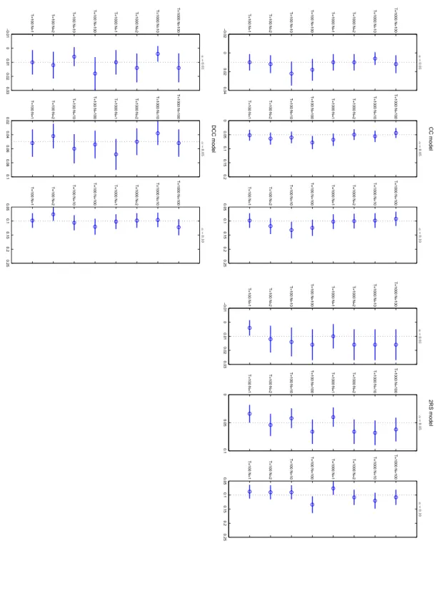
We compare rejection probabilities under the null, based on 500 simulated data sets per scenario. For each data set, the bootstrapped p-value is computed using 500 replications. Results are re-ported in Figure 1. We display, for various N and T , the average and the 95% confidence bands of the frequency that the test rejects the null (under H0) at the 1%, 5% and 10% significance
lev-els. Figure 1 indicates that the size seems correct for the three DGPs, including the two DGPs involving different time-varying dependence structures.
3.2. Power of the test as the number of seriesN (all with wrongfully specified marginals) increases In order to measure the power of our test procedure, and the possible gain in power obtained with a larger number of time series N , we consider the constant correlation (CC) model, where we generate data sets with shifted mean µ > 0 of the marginal distributions ranging from 0 to 0.5, whereas we wrongfully assume µ = 0 in the PITs (i.e., in ˆFt|t−1,i(yti) and ˆft|t−1,i(u) in (2)).
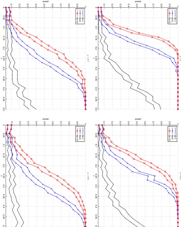
We simulate 500 data sets, where each time we use 500 simulated data sets in our bootstrap test procedure. We consider T = 100 observations for N = 1, N = 10 and N = 100. Results are reported in Figure 2, for a cross-correlation of respectively 0, 0.5, 0.7 and 0.9. The bands reports the 95% confidence bands of the frequency of rejection of the null (at the 5% significance level).
As expected, we observe the following two results. First, the power obviously increases as the actual mean µ in the marginal distributions of the DGP are further away from 0. Second, the gain in power from using a larger number of time series N is smaller for higher values of the cross-correlation. This makes sense, since if the cross-correlation tends to 1, then the addition of extra time series (which are then all (scaled) versions of the same time series) does not increase the power of the test. However, the median cross-correlation between daily returns on equities within a stock index (and between different worldwide equity indices) is typically not as high as 0.7 or 0.9, but rather in the neighborhood of 0.5, as can be seen in Figure 4 in the empirical section.
If all cross-correlations are equal to ρ > 0, and if each time series has the same mean µ 6= 0 (whereas the marginal models assume the misspecified mean 0), then the power does not increase to 1 if N → ∞. Intuitively, each additional i-th time series can be explained increasingly well from the previous i − 1 time series, where the additional information in the additional i-th time series decreases to 0. This explains why the difference in power (for ρ = 0.5, 0.7 or 0.9) between N = 1 and N = 10 is substantially larger than the difference in power between N = 10 and N = 100. However, in practice typically not all marginal models of the time series have the same “amount of misspecification” (here incorporated by the value of µ 6= 0 in the DGP).
3.3. Power of the test as the number of series with wrongfully specified marginals (out of ten series) increases
Figure 3 displays the power of our methodology for N = 10 times series, where the marginal distribution is wrongfully specified for M (M = 1, 5, 10) of the N = 10 series. We generate M time series with shifted mean µ > 0 of the marginal distributions ranging from 0 to 0.5, whereas we simulate N − M time series with mean µ = 0.
The increase in power if M increases from 1 to 10 in Figure 3 is larger than the increase in power if N increases from 1 to 10 in Figure 2. The reason is that the number of ‘nuisance’ series N − M (for which the null is correct) decreases from 9 to 0 in Figure 3.
Obviously, even for large numbers of time series, the gain in power from adding even more time series can still be substantial if the models for the added time series suffer from substantial misspecification that was not present in the models for the other time series. Therefore, if one desires to test for the validity of a set of marginal models, it is obviously recommended to test for the validity of all these marginal models, which may give substantially higher power than testing for the validity of a subset of the models, even if all the time series are highly correlated.
4. Empirical application: Backtesting GARCH models on various equity universes
Investigation of volatility dynamics has attracted many academics and practitioners, as this is of substantial importance for risk management, derivatives pricing and portfolio optimization. Since the seminal paper by Bollerslev (1986), GARCH-type models have been widely used in financial econometrics for the forecasting of volatility. These are nowadays standard models in risk management: they are easy to understand and interpret and available in many statistical packages. For a review on GARCH models we refer the reader to Bollerslev et al. (1992) and Bollerslev et al. (1994).
In our application, we consider the AR(1)-GJR(1,1) specification for the log-returns {rt}:
rt = µ + ρ rt−1+ ηt (t = 1, . . . , T ) ηt = σtεt εt ∼ i.i.d. fε σt2 = ω + (α + γ I{ut−1 ≤ 0}) u2t−1+ β σ 2 t−1, (13)
where ω > 0 and α, γ, β ≥ 0 to ensure a positive conditional variance. I{} denotes the indicator function, whose value is one if the constraint holds and zero otherwise. No constraints have been imposed to ensure covariance stationarity; however, as a sensitivity analysis we have repeated the whole study with additional covariance stationarity constraints, which yielded approximately the same results with qualitatively equal conclusions. Another sensitivity analysis with the inclusion of ‘variance targeting’, where the unconditional variance in the GARCH model is set equal to the sample variance – reducing the number of parameters to be estimated by one, led to similar results. The symmetric GARCH model results by imposing γ = 0. For the distribution fε, we
consider the simple Gaussian and Student-t distributions, together with a non-parametric Gaussian kernel estimator. The Student-t distribution is probably the most commonly used alternative to the Gaussian for modeling stock returns and allows modeling fatter tails than the Gaussian. The
kernel approach gives a non-parametric alternative which can deal with skewness and fat tails in a convenient manner.
Models are fitted by quasi maximum likelihood. For the non-parametric model, the bandwidth is selected by the rule-of-thumb of Silverman (1986) on the residuals of the quasi maximum like-lihood fit; alternative bandwidth choices lead to similar results. We rely on the rolling-window approach where 1000 log-returns – i.e., approximately four trading years – are used to estimate the models. Similar results were obtained for windows of 750 and 1500 observations. Then, the next log-return is used as a forecasting window. The model parameters’ estimates are updated every day.
We test the performance of the models on several universes: (i) a set of nine international stock market indices: the S&P 500 (US), FTSE 100 (UK), CAC 40 (France), DAX 30 (Germany), MIBTel 30 (Italy), Toronton SE 300 (Canada), AORD All ordinaries index (Australia), TSEC weighted index (Taiwan) and Hang Seng (Hong Kong); (ii) equity universe of the DAX 30 index (as of June 2013); (iii) equity universe of the Eurostoxx 50 index (as of June 2013); (iv) equity universe of the S&P 100 index (as of June 2013). For all data sets, we take the daily log-return series defined by yt
.
= log(Pt) − log(Pt−1), where Ptis the adjusted closing price (index) on day t.
The period ranges from January 1990 to June 2013. Data are downloaded from Datastream. The data are filtered for liquidity following Lesmond et al. (1999). In particular, we remove the time series with less than 1500 data points history, with more than 10% of zero returns and more than two trading weeks of constant price. This filtering approach reduces the databases of all universe. More precisely this leads to (i) 9 equity indices, (ii) 24 equities for the DAX, (iii) 39 equities for the Eurostoxx 50, and (iv) 85 equities for the S&P 100. The numbers of observations also vary among the universes. We have respectively 3824 observations for the nine indices, 3367 for the DAX 30, 3549 for the Eurostoxx 50 and 3348 for the S&P 100.
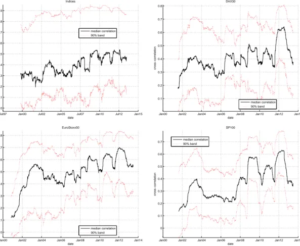
In Figure 4 we display the median (and 5th and 95th percentiles) of the one-year rolling win-dow correlation of the daily log-returns for the four considered universes. Although the cross-correlations vary over time, the median cross-correlation remains closer to (and often below) 0.5 than to 0.7 or 0.9. Hence we expect that our bootstrap test procedure will have a reasonable to good power to detect invalid specifications of the marginal models.
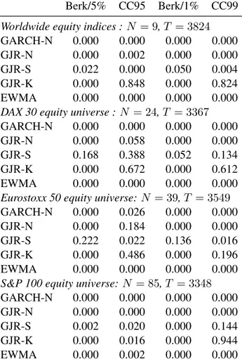
We perform our bootstrap test procedure for the extension of the test of Berkowitz (2001), suggested by Christoffersen and Pelletier (2004), with a specific focus on the left tail (with α = 0.05 and α = 0.01). And we test for correct conditional coverage of the 95% and 99% Value-at-Risk, using the test of Christoffersen (1998). Results for the four universes are reported in Table 1.
The GJR model with Student-t innovations seems the best model. For the N = 24 equities in the DAX 30 and the N = 39 equities in the Eurostoxx 50 indices it is not rejected at a significance level of 5% and 1%, respectively. The other models have at least two p-values of 0.0000 (for the two Berkowitz tests) for each of the four universes. The p-values of 0.000 for the correct conditional coverage test of the 99% Value-at-Risk, which is known to have low power for a univariate time series, reflect the gain in power of our bootstrap test procedure for multiple time series.
4.1. Pre-crisis, crisis and post-crisis periods
The forecast sample period covers the financial crisis of 2008. The performance of the mod-els may vary between the financial-crisis period and the pre-crisis and post-crisis periods. It is important to know if the rejection of most of the models’ forecasts can be ascribed to the crisis period only, or not. We thus present a comparison of the models’ forecasting performance between the crisis period (September 2007 to February 2009), pre-crisis (January 2005-August 2007) and post-crisis period (March 2009 to June 2011); see Ardia and Boudt (2013). Results are reported in Table 2, which shows that the rejection of the density forecasts from the GARCH(1,1) and GJR(1,1) models with Gaussian innovations, the GJR(1,1) model with Gaussian kernel density estimate for the innovations, and the exponentially weighted moving average (EWMA) for the variance estimate is not only due to the crisis period. Also for the pre-crisis and post-crisis sub-periods the validity of these forecasts is rejected. On the other hand, the GJR model with Student-t distributed innovations is rejected for the crisis period, also for the DAX 30 and Eurostoxx 50 uni-verses for which it was not rejected for the whole period (due to its good performance in the pre-crisis period). Therefore, none of the marginal models seems appropriate in the crisis sub-period. This stresses the usefulness of our bootstrap test procedure, since it enables us to perform a relatively powerful test, while focusing on a relatively short (crisis) sub-period of 18 months, in the context of tests for correct conditional coverage which are known to have relatively low power for univariate time series.
5. Possible extensions of the procedure and the applications
In this section, we make several remarks on further possibilities regarding the novel test proce-dure. First, the procedure can easily cope with situations in which the time series are not observed in exactly the same periods. If for some of the time series the PIT is not observed in the first part of the period, then one simply includes missing values or ‘not-a-number’ (NaN or NA) values for the corresponding elements in these rows of the matrices X and R. For the simulated data sets under the null, the NaN values are simply discarded when computing the test statistic for a column, so that the test statistic is computed for a consecutive time series.
Second, the replications in our bootstrap test procedure (i.e., the bootstrapped data sets) are independent, and the test statistics for each time series are computed separately. These two prop-erties facilitate parallel implementation on multiple CPUs or GPUs. Such an implementation may enormously reduce the required computing time, so that one can consider larger universes of stocks within a reasonable amount of computing time. Or alternatively, this enables the use of rather time consuming tests for each time series, such as a bootstrap test procedure for the validity of the Ex-pected Shortfall or Cram´er-von Mises tests. This would then lead to a ‘bootstrap within bootstrap’ test.
Third, it is also possible to add different related test statistics for the same time series, in order to produce one joint test statistic (and corresponding p-value). For example, in our empirical application we could add the four test statistics (of the two Berkowitz tests and the two conditional coverage tests) for each time series to construct one p-value that summarizes the four p-values in Table 1 or Table 2. If in each data set that is simulated under the null these four test statistics are
computed from the same column of simulated PIT values, then the simulated distribution under the null automatically takes into account the dependence between the four test statistics.
Fourth, our proposed method is also applicable if T < N (for example, if one wants to test the validity of a large number of marginal models over a very short period, such as a few days around a crash). In such cases, it would even be difficult to compute a usable covariance matrix.
Fifth, our method can be used to ‘summarize’ a set of p-values for the validity of models for multiple data sets – with which existing papers in the literature may conclude in order to ‘prove’ the validity of the proposed model – in one ‘summarizing p-value’.
Sixth, the method can be used to investigate the effect of the particular dependence of a given data set on a procedure which implicitly assumes independence (or a ‘limited’ type of dependence such as independence between a large enough number of subsets), – an assumption that may be substantially violated by e.g. time series of asset returns. One important example is the false discovery rate (FDR) methodology of Storey (2002). For example, we can investigate how the estimated percentage of correct models (and the confidence interval for this percentage) is affected, under the assumption that all models are correct or under various assumptions on the percentage and nature of misspecified models, where a block bootstrap extension of our method may be used for the latter. This may facilitate the generation of more robust results for the false discovery rate methodology in case of highly dependent time series. Note that in the case of highly dependent time series, we do not have independently uniformly distributed p-values under the null hypothesis, where the latter basically forms the underlying principle of the false discovery rate methodology. Storey and Tibshirani (2003) discuss the FDR under different types of dependence. Under their most general assumptions on the dependence their estimator is (conservatively) biased. Further, they consider DNA data, which arguably have a substantially different dependence structure than e.g. time series in economics and finance.
6. Conclusion
We have introduced a novel simulation-based methodology to test the validity of a set of marginal time series models, where the dependence structure between the time series is taken ‘directly’ from the observed data. We have illustrated its correct size and its power for typically realistic levels of cross-correlation, and shown its potential usefulness in empirical applications involving GARCH-type models for daily returns on stocks or stock indices. We have also shown several possible extensions of the procedure and the applications, which we will consider in future research.
−0.02 0 0.02 0.04 T=100 N=1 T=100 N=2 T=100 N=10 T=100 N=100 T=1000 N=1 T=1000 N=2 T=1000 N=10 T=1000 N=100 α = 0 .0 1 0 0.05 0.1 0.15 0.2 T=100 N=1 T=100 N=2 T=100 N=10 T=100 N=100 T=1000 N=1 T=1000 N=2 T=1000 N=10 T=1000 N=100 α = 0 .0 5 0.05 0.1 0.15 0.2 0.25 T=100 N=1 T=100 N=2 T=100 N=10 T=100 N=100 T=1000 N=1 T=1000 N=2 T=1000 N=10 T=1000 N=100 α = 0 .1 0 CC model −0.01 0 0.01 0.02 0.03 T=100 N=1 T=100 N=2 T=100 N=10 T=100 N=100 T=1000 N=1 T=1000 N=2 T=1000 N=10 T=1000 N=100 α = 0 .0 1 0 0.05 0.1 T=100 N=1 T=100 N=2 T=100 N=10 T=100 N=100 T=1000 N=1 T=1000 N=2 T=1000 N=10 T=1000 N=100 α = 0 .0 5 0.05 0.1 0.15 0.2 0.25 T=100 N=1 T=100 N=2 T=100 N=10 T=100 N=100 T=1000 N=1 T=1000 N=2 T=1000 N=10 T=1000 N=100 α = 0 .1 0 2RS model −0.01 0 0.01 0.02 0.03 T=100 N=1 T=100 N=2 T=100 N=10 T=100 N=100 T=1000 N=1 T=1000 N=2 T=1000 N=10 T=1000 N=100 α = 0 .0 1 0.02 0.04 0.06 0.08 0.1 T=100 N=1 T=100 N=2 T=100 N=10 T=100 N=100 T=1000 N=1 T=1000 N=2 T=1000 N=10 T=1000 N=100 α = 0 .0 5 0.05 0.1 0.15 0.2 0.25 T=100 N=1 T=100 N=2 T=100 N=10 T=100 N=100 T=1000 N=1 T=1000 N=2 T=1000 N=10 T=1000 N=100 α = 0 .1 0 DCC model Figure 1: Size results for the constant correlation model (CC, top-le ft), the tw o-re gime M ark o v switching correlation model (2RS, top-right) and the dynamic conditional correlation (DCC, bottom-left). V arious sample sizes T and numbers of time series N are considered for 500 Monte Carlo replications. The plots display the av erage and the 95% confidence bands of the frequenc y that the null h ypothesis is rejected, at the 1% (left), 5% (middle) and 10% (right) significance le v els. F or each simulated data set, the number of bootstrap replications in the test is set to 500.
0 0.05 0.1 0.15 0.2 0.25 0.3 0.35 0.4 0.45 0.5 0.1 0.2 0.3 0.4 0.5 0.6 0.7 0.8 0.9 1 µ power ρ = 0 N=1 N=10 N=100 0 0.05 0.1 0.15 0.2 0.25 0.3 0.35 0.4 0.45 0.5 0.1 0.2 0.3 0.4 0.5 0.6 0.7 0.8 0.9 1 µ power ρ = 0 .5 N=1 N=10 N=100 0 0.05 0.1 0.15 0.2 0.25 0.3 0.35 0.4 0.45 0.5 0.1 0.2 0.3 0.4 0.5 0.6 0.7 0.8 0.9 1 µ power ρ = 0 .7 N=1 N=10 N=100 0 0.05 0.1 0.15 0.2 0.25 0.3 0.35 0.4 0.45 0.5 0.1 0.2 0.3 0.4 0.5 0.6 0.7 0.8 0.9 1 µ power ρ = 0 .9 N=1 N=10 N=100 2: Po wer results for the constant correlation (CC) model with shifted mean µ > 0 of the mar ginal distrib utions ranging from 0 to 0.5, with correlation of ρ = 0 (top-left), ρ = 0 .5 (top-right), ρ = 0 .7 (bottom-left) and ρ = 0 .9 (bottom-right), for T = 100 observ ations and v arious numbers of time N . The plot displays the 95% confidence bands of the frequenc y of rejecting the null as a function of the shifted mean µ . The number of Monte Carlo is set to one 500, where each time we use 500 bootstrap replications in our test procedure.
0 0.05 0.1 0.15 0.2 0.25 0.3 0.35 0.4 0.45 0.5 0.1 0.2 0.3 0.4 0.5 0.6 0.7 0.8 0.9 1 µ power ρ = 0 M=1 M=5 M=10 0 0.05 0.1 0.15 0.2 0.25 0.3 0.35 0.4 0.45 0.5 0.1 0.2 0.3 0.4 0.5 0.6 0.7 0.8 0.9 1 µ power ρ = 0 .5 M=1 M=5 M=10 0 0.05 0.1 0.15 0.2 0.25 0.3 0.35 0.4 0.45 0.5 0.1 0.2 0.3 0.4 0.5 0.6 0.7 0.8 0.9 1 µ power ρ = 0 .7 M=1 M=5 M=10 0 0.05 0.1 0.15 0.2 0.25 0.3 0.35 0.4 0.45 0.5 0.1 0.2 0.3 0.4 0.5 0.6 0.7 0.8 0.9 1 µ power ρ = 0 .9 M=1 M=5 M=10 Figure 3: Po wer results for the constant correlation (CC) model with shifted mean µ > 0 of the mar ginal distrib utions ranging from 0 to 0.5 for M (M = 1 ,5 ,10 ) out of N = 10 series, and µ = 0 for the remaining N − M series. The correlation v alues of ρ = 0 (top-left), ρ = 0 .5 (top-right), ρ = 0 .7 (bottom-left) and ρ = 0 .9 (bottom-right) are considered for T = 100 observ ations and v arious number s of time series N . The plot dis plays the 95% confidence bands of the frequenc y of rejecting the null as a function of the shifted mean µ . The number of Monte Carlo replications is set to one 500, where each time we use 500 bootstrap replications in our test procedure.
Jul97 Jan00 Jul02 Jan05 Jul07 Jan10 Jul12 Jan15 0 0.1 0.2 0.3 0.4 0.5 0.6 0.7 0.8 0.9 date cross−correlation Indices median correlation 90% band
Jan00 Jan02 Jan04 Jan06 Jan08 Jan10 Jan12 Jan14 0.1 0.2 0.3 0.4 0.5 0.6 0.7 0.8 date cross−correlation DAX30 median correlation 90% band
Jan00 Jan02 Jan04 Jan06 Jan08 Jan10 Jan12 Jan14 0 0.1 0.2 0.3 0.4 0.5 0.6 0.7 0.8 date cross−correlation EuroStoxx50 median correlation 90% band
Jan00 Jan02 Jan04 Jan06 Jan08 Jan10 Jan12 Jan14 0 0.1 0.2 0.3 0.4 0.5 0.6 0.7 date cross−correlation SP100 median correlation 90% band
Figure 4: One-year rolling window cross-correlation of daily log-returns. Top-left: universe of nine stock indices, top-right: DAX 30 equities, bottom-left: Eurostoxx 50 equities, bottom-top-right: S&P 100 equities. Solid line reports the median value of all the cross-correlations while the dotted lines report the 5th and 95th percentiles of the distribution of cross-correlations. The date in the horizontal axis indicates the end of the one-year rolling window.
Berk/5% CC95 Berk/1% CC99 Worldwide equity indices :N = 9, T = 3824
GARCH-N 0.000 0.000 0.000 0.000
GJR-N 0.000 0.002 0.000 0.000
GJR-S 0.022 0.000 0.050 0.004
GJR-K 0.000 0.848 0.000 0.824
EWMA 0.000 0.000 0.000 0.000
DAX 30 equity universe :N = 24, T = 3367
GARCH-N 0.000 0.000 0.000 0.000
GJR-N 0.000 0.058 0.000 0.000
GJR-S 0.168 0.388 0.052 0.134
GJR-K 0.000 0.672 0.000 0.612
EWMA 0.000 0.000 0.000 0.000
Eurostoxx 50 equity universe:N = 39, T = 3549
GARCH-N 0.000 0.026 0.000 0.000
GJR-N 0.000 0.184 0.000 0.000
GJR-S 0.222 0.022 0.136 0.016
GJR-K 0.000 0.486 0.000 0.196
EWMA 0.000 0.000 0.000 0.000
S&P 100 equity universe:N = 85, T = 3348
GARCH-N 0.000 0.000 0.000 0.000
GJR-N 0.000 0.000 0.000 0.000
GJR-S 0.002 0.020 0.000 0.144
GJR-K 0.000 0.016 0.000 0.944
EWMA 0.000 0.002 0.000 0.000
Table 1: Performance results for the whole considered period. Bootstrappedp-values for the 5% lower tail (Berk/5%) and 1% lower tail (Berk/1%) test of Christoffersen and Pelletier (2004), which extends Berkowitz (2001), and for the conditional coverage test of Christoffersen (1998) for the VaR95 (CC95) and VaR99 (CC99). All models contain an AR(1) part. GARCH-N: symmetric GARCH(1,1) with Gaussian innovations; GJR-N: asymmetric asymmetric GJR(1,1) with Gaussian innovations; GJR-S: asymmetric GJR(1,1) with Student-t innovations; GJR-K: GJR(1,1) with Gaussian kernel density estimate for the innovations. EWMA denotes the exponentially weighted moving average for the variance estimate, where a Gaussian distribution is assumed for the innovations. The bootstrap test is computed with 500 replications.
Pr e-crisis Berk/5% CC95 Berk/1% CC99 W orldwide equity indices : N = 9 GARCH-N 0.000 0.444 0.000 0.000 GJR-N 0.000 0.952 0.000 0.000 GJR-S 0.794 0.513 0.000 0.370 GJR-K 0.000 1.000 0.000 1.000 EWMA 0.000 0.000 0.000 0.000 D AX 30 equity univer se : N = 24 GARCH-N 0.000 0.000 0.000 0.002 GJR-N 0.000 0.010 0.000 0.004 GJR-S 0.206 0.150 0.316 0.364 GJR-K 0.000 0.034 0.000 0.608 EWMA 0.000 0.012 0.000 0.000 Eur ostoxx 50 equity univer se: N = 39 GARCH-N 0.000 0.002 0.000 0.000 GJR-N 0.000 0.032 0.000 0.002 GJR-S 0.420 0.160 0.342 0.134 GJR-K 0.000 0.030 0.000 0.426 EWMA 0.000 0.040 0.000 0.000 S&P 100 equity univer se: N = 85 GARCH-N 0.000 0.000 0.000 0.000 GJR-N 0.000 0.000 0.000 0.000 GJR-S 0.008 0.000 0.000 0.024 GJR-K 0.000 0.000 0.000 0.436 EWMA 0.000 0.002 0.000 0.000 Crisis Berk/5% CC95 Berk/1% CC99 W orldwide 0.000 0.000 0.000 0.000 0.000 0.000 0.002 0.000 0.192 0.000 0.486 0.000 0.016 0.000 0.232 0.022 0.000 0.000 0.000 0.000 D AX 30 0.000 0.000 0.000 0.000 0.000 0.000 0.000 0.000 0.048 0.000 0.156 0.000 0.000 0.000 0.000 0.000 0.000 0.000 0.000 0.000 Eur ostoxx 50 0.000 0.000 0.000 0.000 0.000 0.000 0.000 0.000 0.084 0.000 0.396 0.000 0.000 0.000 0.000 0.000 0.000 0.004 0.000 0.000 S&P 100 0.000 0.000 0.000 0.000 0.000 0.000 0.000 0.000 0.114 0.000 0.328 0.000 0.000 0.000 0.000 0.000 0.000 0.020 0.000 0.000 P ost-crisis Berk/5% CC95 Berk/1% CC99 W orldwide 0.000 0.216 0.004 0.000 0.000 0.158 0.018 0.000 0.492 0.054 0.680 0.184 0.184 0.270 0.002 0.604 0.000 0.000 0.000 0.000 D AX 30 0.000 0.010 0.000 0.382 0.000 0.016 0.000 0.310 0.426 0.328 0.146 0.800 0.000 0.040 0.000 0.488 0.000 0.234 0.000 0.000 Eur ostoxx 50 0.000 0.322 0.000 0.004 0.000 0.234 0.000 0.004 0.474 0.188 0.000 0.240 0.000 0.282 0.000 0.694 0.000 0.024 0.000 0.000 S&P 100 0.000 0.004 0.000 0.050 0.000 0.012 0.000 0.178 0.168 0.064 0.080 0.748 0.000 0.014 0.000 0.718 0.000 0.296 0.000 0.000 able 2: Performance results for the pre-crisis, crisis and post-crisis sub-periods. Bootstrapped p -v alues for the 5% lo wer tail (Berk/5%) and 1% lo wer tail test of Christof fersen and Pelletier (2004), which extends Berk o witz (2001), and for the conditional co ver a g e test of Christof fersen (1998) for the aR95 (CC95) and V aR99 (CC99). All models contain an AR(1) part. GARCH-N: symmetric GARCH(1,1) with Gaussian inno v ations; GJR-N: asymmetric with Gaussian inno v ations; GJR-S: asymmetric GJR(1,1) with Student-t inno v ations; GJR-K: asymmetric GJR(1,1) with Gaussian k ernel density for the inno v ations. EWMA denotes the exponentially weighted mo ving av erage for the v ariance estimate, where a Gaussian distrib ution is assumed the inno v ations. The bootstrap test is computed with 500 replications. The windo w sizes are 2305, 1848, 2030 and 1829 for the pre-crisis period for the uni v erses, 370 for the crisis period and 1149 for the post-crisis period.
References
Ardia, D., Boudt, K., 2013. Reconsidering Funds of Hedge Funds: The Financial Crisis and Best Practices in UCITS, Tail Risk, Performance, and Due Diligence. Academic Press: Elsevier Inc, Ch. The Short-Run Persistence of Performance in Funds of Hedge Funds, pp. 289–301.
Barras, L., Scaillet, O., Wermers, R., 2010. False discoveries in mutual fund performance: Measuring luck in estimated alphas. Journal of Finance 65, 179–216.
Berkowitz, J., 2001. Testing density forecasts, with applications to risk management. Journal of Business & Economic Statistics 19 (4), 465–474.
Bollerslev, T., 1986. Generalized autoregressive conditional heteroskedasticity. Journal of Econometrics 31 (3), 307– 327.
Bollerslev, T., Chou, R. Y., Kroner, K., 1992. ARCH modeling in finance: A review of the theory and empirical evidence. Journal of Econometrics 52 (1–2), 5–59.
Bollerslev, T., Engle, R. F., Nelson, D. B., 1994. ARCH models. In: Handbook of Econometrics. North Holland, Ch. 49, pp. 2959–3038.
Christoffersen, P. F., 1998. Evaluating interval forecasts. International Economic Review 39 (4), 841–862.
Christoffersen, P. F., Pelletier, D., 2004. Backtesting Value-at-Risk: A duration-based approach. Journal of Financial Econometrics 2 (1), 84–108.
Diebold, F. X., Gunther, T. A., Tay, A. S., 1998. Evaluating density forecasts with applications to financial risk management. International Economic Review 39 (4), 863–883.
Holm, S., 1979. A simple sequentially rejective multiple test procedure. Scandinavian Journal of Statistics 6 (2), 65–70.
Lesmond, D. A., Ogden, Joseph, P., Trzinka, C. A., 1999. A new estimate of transaction costs. The Review of Financial Studies 12 (5), 1113–1141.
Rosenblatt, M., 1952. Remarks on a multivariate transformation. Annals of Mathematical Statistics 23, 470–472. Silverman, B. W., 1986. Density Estimation for Statistics and Data Analysis, 1st Edition. Chapman and Hall, New
York, USA.
Storey, J., 2002. A direct approach to false discovery rates. Journal of the Royal Statistical Society B 64, 479–498. Storey, J., Tibshirani, R., 2003. Statistical significance for genome-wide studies. Proceedings of the National Academy
of Sciences 100, 9440–9445.
ˇSid´ak, Z. K., 1967. Rectangular confidence regions for the means of multivariate normal distributions. Journal of the American Statistical Association 62 (318), 626–633.
Appendix A. MATLAB implementation
In MATLAB the T × N matrix R of rank numbers is easily computed (from the T × N matrix X of PIT values) by merely two lines of code (using Hungarian notation with i for integer, v for vector and m for matrix):
[mSortedX, mInverseR] = sort(mX);
[mOneToT, mR] = sort(mInverseR);
The second output of MATLAB’s sort command contains the ‘inverse’ rank numbers (indicating which element of X corresponds to each rank number instead of which rank number corresponds to each element): mSortedX equals mX(mInverseR), and mOneToT equals mInverseR(mR), where all N columns of mOneToT are equal to (1, 2, . . . , T )0.
The matrix X is easily simulated under H0 by merely three lines of code:
vV = random(’unid’, iT, iT, 1);
mS = mR(vV, :);