Short-term unit commitment and loading problem
Sara S´
eguin
GERAD & Department of Mathematics and Industrial Engineering
Polytechnique Montr´
eal
Montr´
eal (Qu´
ebec) Canada, H3C 3A7
[email protected]Pascal Cˆ
ot´
e
Rio Tinto Alcan
Saguenay (Qu´
ebec) Canada, G7S 4R5
[email protected]Charles Audet
GERAD & Department of Mathematics and Industrial Engineering
Polytechnique Montr´
eal
Montr´
eal (Qu´
ebec) Canada, H3C 3A7
[email protected]Abstract: This paper presents a new method for solving the short-term unit commitment and loading problem of a hydropower system. Dynamic programming is used to compute maximum power output generated by a power plant. This information is then used as input of a two-phase optimization process. The first phase solves the relaxation of a nonlinear mixed-integer program in order to obtain the water discharge, reservoir volume and optimal number of units working at each period in the planning horizon. The second stage solves a linear integer problem to determine which combination of turbines to use at each period. The goal is to maximize total power produced over all periods of the planning horizon which consists of a week divided in hourly periods. Start-up of turbines are penalized. Numerical experiments are conducted on thirty different test cases for two Rio Tinto Alcan power plants with five turbines each.
Key Words: Hydro unit commitment and loading problem, optimization, nonlinear programming, linear integer programming.
Acknowledgments: This work was supported by the FRQNT (Fonds de recherche du Qu´ebec – Nature et technologies), NSERC (Natural Sciences and Engineering Research Council of Canada) and Rio Tinto Alcan. The authors would like to thank Marco Latraverse from Rio Tinto Alcan for his implication and advice throughout this project.
ORIGINAL CITATION: S. S´eguin, P. Cˆot´e, C. Audet, Self-scheduling short-term unit commitment and loading problem, IEEE Transactions on Power Systems, 31(1), 133–142, Jan. 2016. http://dx.doi.org/10.1109/ TPWRS.2014.2383911.
1
Introduction
The planning of hydroelectric systems is complex and requires different optimization processes. A good planning allows to produce more power with the same quantity of water, generating substantial savings for the producer, even with a slight computational improvement [12]. Long-term, medium-term and short-term optimization models are used in order to manage the resources. Long-term optimization follows a 2-3 year planning horizon [5] and establishes future production potential under highly uncertain inflows in the basins. Medium-term optimization [8] is used to plan the reservoir volumes by estimating the quantity of water available for hydroelectric production on a weekly basis. This optimization takes into account the water transfer function between plants, minimum and maximum levels of reservoirs, uncertainty of the inflows and energy demands. Short-term optimization [7] is mandatory to determine how to split the available water volume in an optimal way between the turbines of a plant. Each turbine has a different efficiency curve which means that for the same water discharge the power will differ. The planning horizon is a week divided in hourly periods and the problem consists of finding the optimal water discharge as well as the volume of the reservoir for each plant in order to maximize power production and penalize start-ups of turbines. The present work focuses on short-term optimization.
These optimization problems are difficult to solve since the hydroelectric production functions are non-convex. They are also highly nonlinear and depend on turbine efficiency, net water head that is a nonlinear function of the water discharge and reservoir elevation and finally, water discharge of each unit. Furthermore, turbines have forbidden operating zones, which complicates the problem.
Short-term unit commitment and loading problem have been studied in the past and many researches are still undergoing. Many methods have been proposed to solve the short-term unit commitment and loading problem, including dynamic programming. In [1], a power generation loss function is used to take into account the hydro power efficiency in the dispatch of the plants, but considers the forebay elevation insignificant and neglects the water balance equations. Another approach [22] maximizes basinwide operating efficiency and changes the scheduling of the units only when the energy generation or the water discharges exceed a deadband. These assumptions will cause the optimization solution to differ from the real ones. Formulations of interest must consider tailrace elevations, penstock losses as well as efficiency of the turbines, which are often set aside to simplify the problem. A different manner [3] approximates the influence of the head effect to linearize the power production function, while Ohishini [14] assumes that all units of a hydropower plant are similar and does not consider different power outputs being produced by the units. Another widely used method is the the lagrangian relaxation to separate the linking constraints and solve sub-problems that are easier to compute [4]. However, this method usually causes solutions to be slightly infeasible since the linking constraints are rarely satisfied with the first solutions. Heuristics are then used to obtain a feasible solution. Not only are the methods different, but the choice of the objective function can vary from one method to the other. Another formulation of the problem [11] is to minimize the sum of power losses and solve a relaxed mixed-integer nonlinear problem. Then, a simulation phase is processed to obtain a feasible solution for the relaxed constraints. Once again, a two-phase approach is necessary to obtain a feasible solution. In [18], the plant efficiency is maximized since it is known that water is not used in an efficient way to meet the demand in energy. Nonlinear approaches [6] have been considered, by linearizing the hydro power efficiency of the plants and the water level functions, but do not consider the unit commitment of the plants. Other techniques have been proposed, including genetic algorithms [17], ant algorithms [13] and network flows [15], but they require parameter tuning before obtaining solutions, which is not an issue when using mixed-integer formulations, nonlinear problems or lagrangian relaxations, just to name a few.
This paper presents a new approach for modeling the short-term unit commitment and loading problem that requires a two-phase approach and allows to find a feasible solution at the end of the first stage. The first optimization dispatches generation among plants and seeks to maximize total power production. For each period and each plant, reservoir volume, water discharge and optimal number of units working is determined. The second stage uses this solution to select the optimal unit commitment that, once again, maximizes total power production but also penalizes unit start-ups. The models are then tested on two hydroelectric plants in series.
The paper is organized as follows. Section 1.1 presents the hydroelectric system studied in this paper. Section 2 gives an overview of the problem characteristics and presents characteristics of the short-term optimization problem. Sections3presents the mathematical models developed which are a nonlinear model and a linear integer program. They respectively aim to solve the loading problem as well as the optimal unit commitment problem. Extensive numerical experiments are reported in Section4on thirty test cases for two power plants with five turbines each, and concluding remarks are drawn in Section5.
1.1
Saguenay-Lac-St-Jean hydroelectric system
The models presented in this paper are tested on the Saguenay-Lac-St-Jean hydroelectric system. It is privately owned by Rio Tinto Alcan in the province of Quebec. This company operates aluminum plants in that region and can produce 90% of the energy they need to operate them. The installed capacity is of 3100 M W and is composed of 42 turbines divided in five hydroelectric plants situated on the P´eribonka and Saguenay rivers. Five reservoirs are available and three of them have a stocking capacity of over 2000 hm3. The hydrographic basins cover an area of about 75 000 km2. Energy prices do not need to be taken into account for the short-term unit commitment an loading probelm since Rio Tinto Alcan does not trade their energy on the markets. For the purpose of this paper, the models are tested on two of the five hydroelectric plants since a deterministic model is developed to validate modeling. The plants are Chute-du-Diable and Chute-Savane and they are both composed of five turbines.
Specific constraints related to the Saguenay-Lac-St-Jean system, which is the purpose of this study, need to be taken into account when developing the model. In some cases, the hydroelectric functions are nonconvex and nondifferentiable. For example, the tailrace elevation for a given number of plants can only be obtained by simulation and there are no analytical representation of these functions. A practical, accurate and efficient model in terms of computational time needs to be developed.
1.2
Notation
The following notation is used throughout the paper: k ∈ {1, 2, . . . , K} index of periods
c ∈ {1, 2, . . . , C} index of hydroelectric plants
s ∈ {1, 2, . . . , nck} index of surfaces corresponding to number of active turbines associated to hydroelec-tric plant c
l ∈ {1, 2, . . . , nc
k} index of combinations associated to hydroelectric plant c and period k
t ∈ {1, 2, . . . , mclk} index of turbines associated to combinations l, hydroelectric plant c and period k vc
k volume of plant reservoir c at period k (hm 3) qc
k water discharge at plant c and period k (m3/s) θ start-up penalty for any turbine (M W h) βc
lk power generated by combination l ∈ nck at plant c and period k
yc sk=
1 if surface s is chosen at period k for plant c 0 otherwise sc lkt= 1 if turbine t of combination l for plant c is working at period k 0 otherwise xc lk= 1 if combination l of plant c is chosen at period k 0 otherwise dc tk=
1 if turbine t of plant c is started at period k
χs(vc
k, qkc) power output function for surface s (M W h) δc
k inflow of plant c at period k (m 3/s) wk duration of period k (h)
γ conversion factor from water discharge (m3/s) to volume (hm3) ζk conversion factor to power units (GW h)
vc
min minimal volume of plant c reservoir (hm3) vc
max maximum volume of plant c reservoir (hm3) qc
min minimum water discharge at plant c (m3/s) qc
max maximum water discharge at plant c (m3/s).
2
Short-term unit commitment and loading problem
The short-term unit commitment and loading problems must determine a production plan for each turbine in the system, for each period of the planning horizon considered. The objective is to maximize power production and penalize unit start-ups. This section describes the characteristics of the problem and presents an optimization model that requires a short computational time to solve.
2.1
Problem description
Power produced by a single hydroelectric generator [20] is given by the equation:
P = n(Q) × g × Q × hn (1)
where P is the power output in kW , n(Q) is the turbine-generator overall efficiency, g is the gravitational acceleration in m/s2, Q is the turbine water discharge in m3/s and hn the net water head in m.
For a given turbine, power is a function of the water discharge, the net water head and the efficiency. Gross head is the difference between forebay and tailrace elevation. When water runs in the penstock, friction causes heat dissipation, causing a diminution in energy. This phenomena causes a loss that needs to be considered in the power output calculation. Net water head is obtained from the gross head from which the losses are taken into account. Net water head is computed by:
hn(v, q) = hf(v) − ht(q) − ψ(q) (2)
where v is the volume of the reservoir in m, q is the total water discharge in m3/s, hf is a nonlinear function returning forebay elevation in m, ht is a nonlinear function returning tailrace elevation in m and ψ is a nonlinear function returning friction losses in m.
The focus of this paper are Chute-du-Diable and Chute-Savane plants in the Saguenay-Lac-St-Jean hy-droelectric system. Chute-Savane is situated upstream of the Lac-St-Jean, hence the tailrace elevation of this plant is affected by the level of the lake. A particularity of the system is that there is no analytical representation of the tailrace elevation for this plant. The value can only be calculated by a computer simu-lation. Since power depends on net water head and water discharge, there is no analytical representation of the power output functions. This particularity also deprives us of their derivatives.
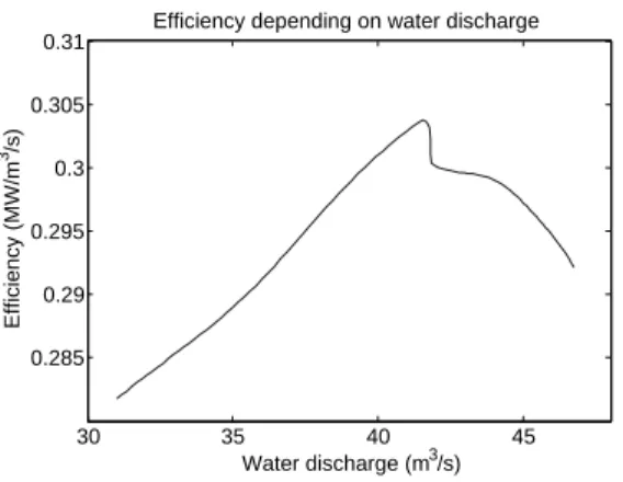
Each turbine possesses its own efficiency curve, causing them to produce different power outputs for the same water discharge and net water head. Also, efficiency depends on water discharge of the turbine. Fig.1
illustrates the efficiency of a turbine as a function of water discharge for a given net water head at the Chute-du-Diable plant.
In Fig.1, the water discharge of 48 m3/s generates the greatest energy and is called maximum flow rate. It also refers to maximum power output that can be produced by the unit. This limit is fixed by the turbine manufacturer. Each turbine is designed to operate at a certain water discharge and when the actual discharge is near this value, power produced by the unit is at its maximum efficiency. When the limit is reached, water
30 35 40 45 0.285 0.29 0.295 0.3 0.305 0.31 Water discharge (m3/s) Efficiency (MW/m 3/s)
Efficiency depending on water discharge
Figure 1: Turbine efficiency as a function of water discharge
needs to be spilled, causing power and efficiency to decrease. Turbines should always be used within their efficiency zones for these reasons.
Another particularity that complicates the problem is the forbidden zones of operations of the turbines [9]. Under certain operating conditions, a vortex may occur in the turbine and create pressure variations. These variations affect power output as well as overall efficiency and vibrations created by these vortices can damage the components of the hydroelectric turbines. These zones are forbidden and turbine are not operated when these conditions are met.
Also, unit restarts should be limited since they shorten equipment life [2]. Each restart can be defined as a number of working hours which causes maintenance of the generating units to occur sooner. Likewise, equipment service life is reduced since it corresponds to working hours. There is also a cost associated to a unit start-up. They take into account the history of expenses in maintenance and repairs in relation with the number of start-ups.
These values are laboriously calculated by Rio Tinto Alcan and become parameters in the optimization models.
One could formulate the power production optimization problem as a linear integer program by discretizing unit water discharge, volumes and total water discharge for each turbine, power plant and period in order to maximize total power production. However, the number of optimization variables would be extremely large. For instance, if total water discharge is discretized from 0 to 900 m3/s, unit water discharge from 0 to 150 m3/s both with steps of 5 m3/s, with 168 hourly periods for a week and volumes from 46 to 394 hm3 discretized in 100 slices, then the number of binary variables would be of the order of 108. Water discharges are discretized every 5 m3/s since it is operationally impossible to obtain a finer precision, and volumes in 100 slices give a good final precision for the Saguenay-Lac-St-Jean hydroelectric system. This suggests that the number of variables required is unrealistic for a real-time application.
2.2
Problem modeling
Power output of a single turbine is a function of two variables of the water discharge and the volume. However, there is a relation between the net water head and the volume of the reservoir. For the remainder of the paper, volume will be used to simplify notation. Total power output of a plant depends on total water discharge, number of working units and active turbines. Efficiency curves are specific for each turbine, hence unit power output is different for the same water discharge. Depending on the number of units working, but also on which units are employed, total power output is different. Instead of working directly with turbines in the model, fewer variables are needed if active turbines are grouped in combinations. For example, for the Chute-du-Diable plant, five turbines are available, but operational restrictions require a minimum of three
active turbines. Table1 lists the sixteen possible combinations. In each column, the numbers represent the actual active turbines.
Table 1: Turbine combinations at Chute-du-Diable
3 active turbines 4 active turbines 5 active turbines
123 145 1234 12345
124 234 1235
125 235 1245
134 245 1345
135 345 2345
For a given water discharge, water volume and active turbines combination, the optimal dispatch of the water between the turbines is obtained by a dynamic programming algorithm. For each discretization of the water discharge and the volume, this algorithm needs to be processed. This means that for every possible combo of water discharge and volume, the algorithm calculates the power output that can be obtained for every combination of active turbines. These values are then used as parameters for the optimization models. A model using combinations of active turbines needs to determine which one to use at each period as well as the volume and the total water discharge. In the linear integer model discussed at the end of Section2.1, the unit water discharge discretization is replaced by the number of combinations. Although the number of variables is significantly less than with the linear model using turbines, it remains too important to be computationally solvable in a reasonable amount of time.
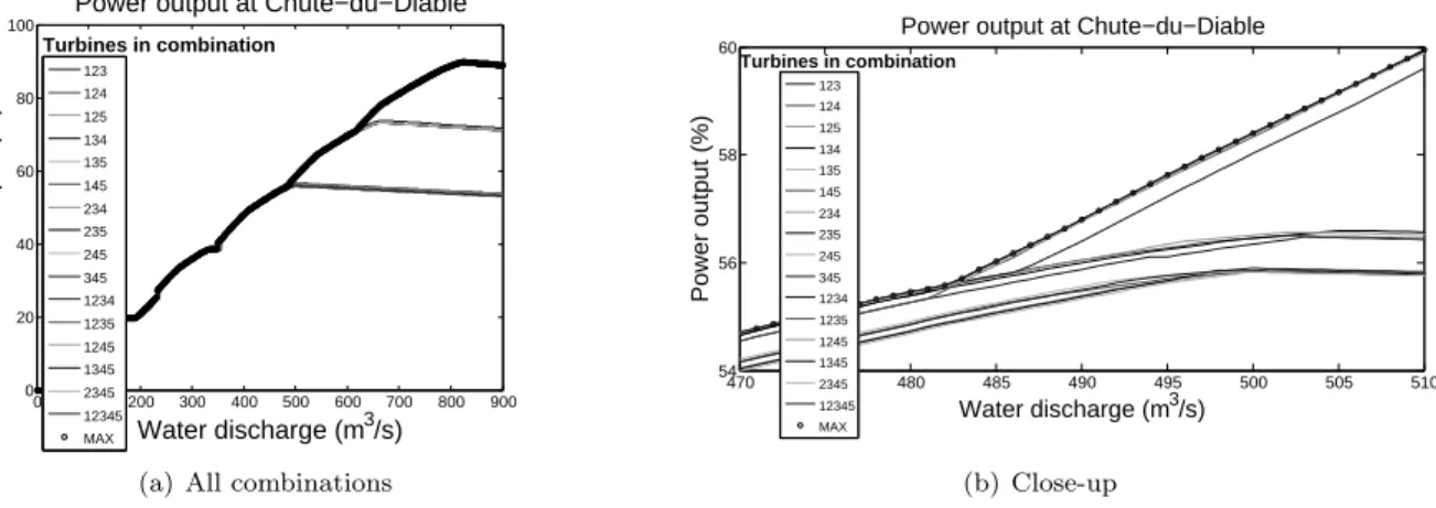
For a given volume and turbine, the power output depends on the water discharge. The same applies to combinations: if turbines in the combination differ, then the total power output will be different. Fig.2(a)
shows curves of the power output depending on the water discharge for all possible combinations at Chute-du-Diable power plant, for a volume of 376 hm3and Fig.2(b)is a close-up. The values are computed by the dynamic programming algorithm.
0 100 200 300 400 500 600 700 800 900 0 20 40 60 80 100 Water discharge (m3/s) Power output (%)
Power output at Chute−du−Diable
Turbines in combination 123 124 125 134 135 145 234 235 245 345 1234 1235 1245 1345 2345 12345 MAX
(a) All combinations
470 475 480 485 490 495 500 505 510 54 56 58 60 Water discharge (m3/s) Power output (%)
Power output at Chute−du−Diable
Turbines in combination 123 124 125 134 135 145 234 235 245 345 1234 1235 1245 1345 2345 12345 MAX (b) Close-up Figure 2: Power output at Chute-du-Diable
Observe that the power output decreases when the maximum efficiency of the turbine combination has been reached. As seen on Fig. 2(a), from 0% to 55%, three turbines are in the combination, from 55% to 75% four turbines are in the combination and five from 0% to 90%. When an extra turbine is added in the combination, maximum efficiency has been reached. These curves could be used to model the problem. Fig.2(a)shows total power output that can be obtained by a combination for each water discharge. The objective of the problem is to maximize total power generation and a new function corresponding to the maximum envelope of all combinations can be created. This new function returns the maximum power that can be generated for a given water discharge, a reservoir volume and a given number of units. It is represented by the bold curve on Fig.2(a).
For each water discharge, maximum power output is used, whatever the combination, which means that from one value of water discharge to the other, the combination can differ. This can be generalized for the discretization of volumes. One hundred discretizations are done, between the minimum and maximum reservoir volume and are shown in Fig.3(a). The interest for this function is that it gives us an upper bound on the optimal value of the problem for a volume and a given water discharge.
0 5 10 0 10 20 30 400 20 40 60 80 100 Volume discretization Power output at Chute−du−Diable
Water discharge discretization
Power output (%)
(a) Surface
Contour plot of power output at Chute−du−Diable
Volume discretization Power output (%) 30 40 50 60 70 24 32 40 48 (b) Contour plot Figure 3: Power output at Chute-du-Diable
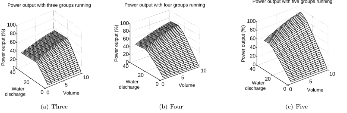
The changes in the number of active turbines in the combination cause a problem for modeling this surface since they correspond to nondifferentiable zones. The contour plot shown in Fig.3(b)illustrates this property. A way to overcome these difficulties is to create a surface for each number of active turbines in the combination. In this case, surfaces with three turbines working, four turbines and five turbines are created, as shown in Fig.4. 0 5 10 0 20 400 20 40 60 80 100 Volume Power output with three groups running
Water discharge Power output (%) (a) Three 0 5 10 0 20 400 20 40 60 80 100 Volume Power output with four groups running
Water discharge Power output (%) (b) Four 0 5 10 0 20 400 20 40 60 80 100 Volume Power output with five groups running
Water discharge
Power output (%)
(c) Five Figure 4: Power output with different number of active turbines
These surfaces are easy to model. The mathematical model must determine one surface per period, giving us at the same time the optimal number of active turbines. These surfaces are valid if the turbines of the plant are available at a given period. Hence, if a turbine is unavailable for a given period, surfaces need to be recalculated without considering the unavailable turbine. Thus, for each plant and each period, the number of surfaces may vary, as well as the surfaces themselves. For instance, if one turbine is unavailable, only the surfaces with three or four active turbines are possible, and if two turbines are unavailable, then only one surface is possible. The dynamic programming algorithm is computed for every number of active turbines in the combination as well as for every combination of unavailable turbines and power outputs are stored in a database. Models then consult the database, depending on possible number of active turbines and available turbines. Unavailable turbines cause the number of combinations as well as the number of surfaces to be reduced.
The volume of available water for production is obtained from the medium-term optimization and is an input to the loading problem, as well as the initial combination of working turbines. The turbines working at the end of a week need to be the initial combination at the beginning of the next week. This initial combination is denoted ˆycskand is a parameter for the short-term unit commitment and loading optimization models.
The use of theses surfaces does not allow us to penalize the start-up of turbines, hence the optimization needs to use a two-stage approach. The first stage is a nonlinear mixed-integer model and returns the water discharge, reservoir volume as well as the number active turbines. The second stage is a linear integer model that determines exactly the combination of turbines to use at each period in order to minimize the start-up of turbine so that power is maximized.
3
Mathematical models
This section presents the mathematical models used to solve the short-term unit commitment and loading problem. The first one distributes generation among plants and the second determines the optimal unit commitment.
3.1
Loading problem
The first optimization consists of a nonlinear mixed-integer program that determines the water discharge, reservoir volume and number of active turbines at each period for each power plant. This model is valid for hydroelectric plants in series. The function χs(vck, q
c
k) corresponds to power output of a given number of active turbines, for a given water discharge and volume. The initial number of active turbines ˆyc
s1is known. Power output is computed with a dynamic programming algorithm, as explained in Section2.2. The number of surfaces per plant and period is given by nc
k. Maximize total power production:
maxX c∈C X k∈K X s∈nc χs(vck, q c k)y c skζk (3) subject to: δk1= v 1 k+1− v 1 k+ γwkq 1 k, ∀k ∈ K\{1} (4) δck= vk+1c − vc k+ γwkq c k+ γwkq c−1 k , ∀k ∈ K\{1}, ∀c = 2, 3, . . . , C (5) X s∈nc k ycsk= 1, ∀c ∈ C, ∀k ∈ K\{1} (6) ys1c = ˆycs1, ∀c ∈ C, ∀s ∈ nc k (7) vcmin≤ vc k≤ v c max, ∀c ∈ C, ∀k ∈ K (8) qcmin≤ qkc ≤ q c max, ∀c ∈ C, ∀k ∈ K (9) qck≥ 0, ∀c ∈ C, ∀k ∈ K (10) vck≥ 0, ∀c ∈ C, ∀k ∈ K (11) yskc ∈ B, ∀c ∈ C, ∀k ∈ K, ∀s ∈ nc k (12) qck, vck∈ R, ∀c ∈ C, ∀k ∈ K. (13)
Constraints (4) and (5) assure that water balance of the plants are met. The values of v1c and vk+1c are known and obtained from the medium-term optimization model. Constraints (6) forces the model to choose only one surface at each period for each plant and constraint (7) feeds the model with the turbines already working at the beginning of the planning horizon. Constraints (8) and (9) represent the physical limits for volume of the reservoirs as well as the water discharge operational limits. Non-negativity of the variables are taken into account by constraints (10) and (11). Finally, (12) imposes binary variables and (13) real variables.
In practice, nonlinear mixed-integer programs require a large amount of computing time when solving since some variables, in this case those associated to the surfaces, are integer variables. Luckily, we can prove that solving the continuous relaxation of the surface variables yc
k of this problem is sufficient to obtain an integer solution on these variables. Solving the relaxed nonlinear problem will return a solution with integer variables, even though imposing integer variables has been omitted.
Proposition 3.1 Solving the relaxation of integer program (3)–(13) leads to an integer solution.
Proof. The proof of the result is done by showing that the matrix of constraints is totally unimodular. Problem (3)–(13) can be re-written as follows:
maxX ω∈Ω X c∈C X k∈K X s∈nc ηωycskζk (14) subject to: X s∈nc k ycsk= 1, ∀c ∈ C, ∀k ∈ K\{1} (15) ys1c = ˆycs1, ∀c ∈ C, ∀s ∈ nc k (16) ycsk∈ B, ∀c ∈ C, ∀k ∈ K, ∀s ∈ nck. (17)
where ηw is the power for ω the feasible set with respect to constraints (4) and (5) and ˆyc
sk is the initial combination of turbines working from the medium-term optimization.
Denote the matrix of coefficients of the constraints for problem (14)–(17) by A. Wolsey [21] shows A is totally unimodular if and only if the following three conditions are satisfied:
1. aij ∈ {+1, −1, 0} ∀i, j.
2. Each column of A contains at most two nonzero coefficients (Pmi=1|aij| ≤ 2).
3. There exists a partition (M1, M2) of the set M of rows of A such that each column j containing two nonzero coefficients satisfies P
i∈M1aij−
P
i∈M2aij = 0.
Condition 1. is satisfied by Equations (15)–(16). Each column of the matrix A has a single element, which imply that Conditions 2. and 3. are satisfied.
Therefore, A is totally unimodular and there is an integer optimal solution of the continuous relaxation.
The following nonlinear relaxed program can be solved, where yc
sk are continuous variable associated to the surfaces.
Maximize total power produced at each period:
maxX c∈C X k∈K X s∈nc χs(vkc, qck)ycskζk (18) subject to: (4) − (5) (19) X s∈nc ycsk≤ 1, ∀c ∈ C, ∀k ∈ K (20) (7) − (11) (21) ycsk≥ 0, ∀c ∈ C, ∀k ∈ K, ∀s ∈ nck (22) ycsk∈ R, ∀c ∈ C, ∀k ∈ K, ∀s ∈ n c k. (23)
Constraints remain the same, except for (20) that becomes an inequality and (22) and (23) that are the non-negativity constraints for continuous variables associated to the choice of the surface.
3.2
Unit commitment
The solution produced by the nonlinear relaxed program is an input to the unit commitment problem. The unit commitment model is a linear integer program and it determines the exact combination of turbines to use in order to maximize total power production at each period and penalize start-up of turbines. The initial combination of working turbines ˆxc
lk is known. The number of combinations for a given period and power plant is given by nc
k and turbines in the combination for a given period and plant by mclk. The optimization problem maximizes power produced and penalizes turbine start-ups:
maxX c∈C X k∈K X l∈nc k βclkxclkζk−X c∈C X k∈K X t∈mc lk X l∈nc k dctkθ (24) subject to: X l∈nc k xclk= 1, ∀c ∈ C, ∀k ∈ K\{1} (25) xclksclkt− xclk−1sclk−1t≤ dctk, ∀c ∈ C, ∀k ∈ K, ∀l ∈ nck, ∀t ∈ mclk (26) xcl1= ˆxcl1, ∀c ∈ C, ∀l ∈ nc k (27) xclk∈ B, ∀c ∈ C, ∀k ∈ K, ∀l ∈ nc k (28) dckt∈ B, ∀c ∈ C, ∀k ∈ K, ∀l ∈ nc k, ∀t ∈ m c lk. (29)
The constraints (25) ensure that only one combination is chosen at each period. Constraints (26) are the linking constraints between start-up variables and combination choice. Constraints (27) force the initial combination of turbines working. Finally, constraints (28) and (29) are the declaration of binary variables.
4
Computational results
The mathematical models of Sections 3.1 and 3.2 are tested on two of the five hydroelectric plants that compose the Saguenay-Lac-St-Jean hydroelectric system. These two plants, du-Diable and Chute-Savane, are in series and both have five turbines. They were chosen since they are the smallest sub-system with two plants in series and the motivation is to validate the optimization developed before expanding to the whole hydroelectric system. Also, the models developed are deterministic and the aim of subsequent studies will be to consider uncertainty in the weather forecasts. Chute-du-Diable has an installed capacity of 224 M W , a gross elevation of 33.5 m and a reservoir of 47 km2. Chute-Savane has an installed capacity of 245 MW, a gross elevation of 33.5 m and a reservoir of 18.5 km2.
The planning horizon of the models is partitioned into 168 hourly periods for one week. Thirty weekly scenarios are tested, all provided from the historical database. Since data is available every two minutes, a mean per hour for the water discharge and the volume of the reservoirs is calculated in order to compare results. Initial volume, final volume and initial combination of working turbines are provided to the model to make the best possible comparison. The same starting point, in the middle of volume and water discharge discretizations is given to the model as an initial solution.
Inflows of the basins are assumed known and the computed model is deterministic. Once again, data is available every two minutes, so a mean per hour for the water inflow in the basin is calculated to feed the mathematical model.
The Ipopt [19] nonlinear solver is used for the first nonlinear program and Xpress-MP [16] for the second linear program. Numerical experiments are conducted with an Intel Xeon Processor E5-2650, with 8 cores at 2 GHz and 61 Go of RAM memory. The nonlinear program has a total of 1680 real variables and 674 constraints. For the second linear integer program, 7056 binary variables and 26918 constraints are necessary. The number of constraints and variables are obtained for the worst case, meaning 16 combinations of active turbines are possible at every period. The number of variables and constraints for the second model will be less if some turbines are unavailable due to maintenance or repair at certain periods.
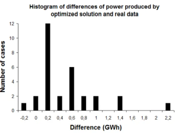
Numerical comparisons of our approach versus the real values show an improvement on 27 out of the 30 test cases, ranging from 0.002 GW h to 2.145 GW h. The average improvement over all cases is of 0.4 GW h. In the province of Quebec, a 1 M W h earning represents roughly 40$ in savings for the producer. In this particular case, an improvement of 0.4 GW h translates into 832 000$ savings for a year.
Our approach is slightly sensitive to the starting point value. We observed that for the three cases in which our approach did not improve the solution, a better solution was found by changing the starting point. In future work we plan to study more thoroughly this behaviour.
The computational time to solve the unit commitment model is very low. The loading problem takes an average of 1.41 seconds and the longest time is 7.71 seconds. This case has the particularity of being the only one with certain periods having two turbines down for maintenance, which causes these periods of having only one possible surface to optimize.
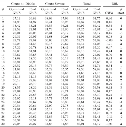
Results obtained with the same initial solution are shown in Table 2. For each hydroelectric plant, to-tal power, with penalties due to start-ups, both for solution obtained with the optimizer and the historical database are listed. Also, the difference between optimized solutions and the historical database are com-puted. A positive value indicates that the optimizer produces a better solution than reality and a negative value indicates the opposite. Also, the total difference of start-ups of turbines is listed. It is not necessary to list for both power plants since they are, most of the time, equally divided between both of them. A positive difference indicates optimized solution has more starts than real case and a negative difference indicates real case has more starts.
Fig.5is a histogram comparing power gain between optimized solution and real test cases. In twelve out of the thirty test cases, the optimized solution improved the quantity of power produced between 0 and 0.2
Table 2: Total power production with same initial solution
Chute-du-Diable Chute-Savane Total Diff.
# Optimized Real Optimized Real Optimized Real #
GW h GW h GW h GW h GW h GW h GW h start 1 27,12 26,82 38,09 37,93 65,21 64,75 0,46 0 2 31,96 31,97 35,41 35,25 67,37 67,21 0,16 1 3 33,42 33,21 36,55 36,21 69,97 69,42 0,55 -1 4 22,52 22,07 24,73 23,80 47,25 45,87 1,38 0 5 25,01 25,05 28,31 28,12 53,32 53,17 0,15 -3 6 29,36 29,07 31,68 30,98 61,03 60,05 0,98 2 7 22,74 22,87 30,00 29,96 52,74 52,82 -0,08 5 8 32,26 31,56 30,18 29,67 62,44 61,23 1,21 3 9 27,29 26,78 38,38 38,42 65,67 65,20 0,47 1 10 32,06 31,91 36,10 35,52 68,16 67,42 0,74 0 11 36,67 36,68 38,41 38,39 75,07 75,07 0,00 0 12 28,68 28,30 36,59 36,14 65,27 64,44 0,83 0 13 33,94 33,93 38,80 38,72 72,73 72,65 0,08 0 14 26,52 26,15 36,76 36,59 63,28 62,74 0,54 1 15 24,04 23,54 35,29 35,35 59,33 58,88 0,45 1 16 33,80 33,53 37,85 37,63 71,66 71,16 0,50 0 17 31,13 31,13 36,54 36,43 67,67 67,56 0,11 0 18 30,18 29,89 31,84 31,94 62,01 61,83 0,18 2 19 29,10 28,70 31,26 31,37 60,36 60,06 0,29 4 20 28,57 28,26 31,33 31,32 59,90 59,58 0,32 3 21 27,04 26,96 29,80 29,71 56,84 56,67 0,17 1 22 28,17 27,83 30,68 30,27 58,84 58,10 0,75 -4 23 25,05 25,11 27,77 27,57 52,82 52,68 0,14 0 24 33,64 32,67 36,97 35,80 70,61 68,47 2,15 -1 25 20,54 20,64 22,90 22,78 43,44 43,42 0,02 2 26 31,91 31,87 35,14 35,14 67,06 67,01 0,05 -2 27 20,34 20,48 23,41 23,25 43,74 43,73 0,02 3 28 29,48 29,62 32,83 32,79 62,31 62,41 -0,11 -2 29 33,34 33,34 36,68 36,56 70,02 69,90 0,12 1 30 29,08 29,27 31,83 31,85 60,91 61,12 -0,21 3 10
GW h. For ten other cases, the improvement is between 0.2 and 1.0 GW h. Three cases exceed 1.0 GW h and the largest gain is close to 2.2 GW h. In 27 of these cases the improvement is positive, and in the other 3 the improvement is slightly negative.
Figure 5: Histogram of differences of power
4.1
Interpretation of the results
We illustrate the differences between the real and the optimized solutions by analyzing two of the test cases. These cases were selected since one of them proposes a very different production plan than the decisions actually taken at the moment. In fact, they also show that even though the strategy is very different, more power can be produced in the end. Also, fifteen of the cases have more starts with the optimized solution than the real cases, and thirteen generate more power. It is important to notice that not all constraints of the database results are modeled in the optimization problem. In fact, some constraints concerning power production stated in contracts are neglected in this paper, but do not have a major impact on the general results presented in this section. Solutions can be slightly different, but overall results are comparable.
Case 1 fills the reservoir during the week and case 6 has similar volumes at the beginning and the end of the week.
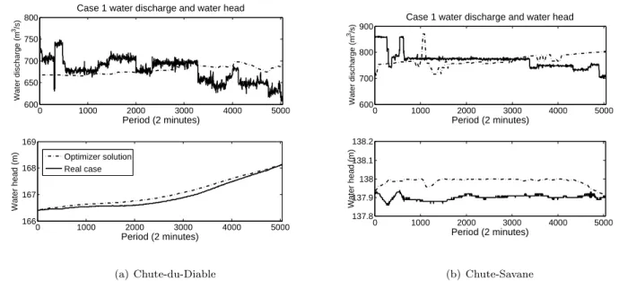
Since power is a two variable function of the net water head and water discharge, both graphs are presented. For Chute-du-Diable and Chute-Savane, a graph of the water discharge comparing optimized solution and reality as well as a graph comparing water heads are displayed for all four cases.
Let us analyze case 1 in details. Fig.6(a)shows the results for Chute-du-Diable power plant. The graphic on top shows the total water discharge of the plant in m3/s and the graphic below shows the net water head in m. The period for both graphs is 2 minutes, as in the historic database. The optimized result over the entire week are transposed every 2 minutes to allow a visual comparison. Even though a mean per hour of the 2 minute inflows has been computed for the optimization, the total volume is equivalent for 2 minutes real results and 1 hour optimized solutions. For each graph, the optimized solution is presented with a dashed line and the real cases with a filled line. Fig.6(b) shows the results for Chute-Savane. The top graphic of Fig.6(a)shows the optimized solution in which the total water discharge at the plant is 670 m3/s during the whole planning horizon. Graphic on the bottom, on Fig.6(a), illustrates the water head is similar throughout all the week for database and optimizer solution. Fig.6(b) on top shows database solution give a constant water discharge of about 780 m3/s with a higher discharge at the beginning of the week, and that optimized solution has also a constant solution with a peak of the water discharge around period 1000. As for the graphic on the bottom, the optimized water head is higher than database results throughout the week. The solution provided by the optimizer produces an improvement of 0.462 GW h.
For case 6, the solutions for both power plants have strategies different than decisions made at that moment. Chute-du-Diable’s reservoir is lowered then filled and Chute-Savane is filled, then lowered and filled once again. Results are presented on Fig.7.
0 1000 2000 3000 4000 5000 600 650 700 750 800 Water discharge (m 3/s)
Case 1 water discharge and water head
Period (2 minutes) 0 1000 2000 3000 4000 5000 166 167 168 169 Period (2 minutes) Water head (m) Optimizer solution Real case (a) Chute-du-Diable 0 1000 2000 3000 4000 5000 600 700 800 900 Water discharge (m 3/s)
Case 1 water discharge and water head
Period (2 minutes) 0 1000 2000 3000 4000 5000 137.8 137.9 138 138.1 138.2 Period (2 minutes) Water head (m) (b) Chute-Savane Figure 6: Case 1 water discharge and water head
0 1000 2000 3000 4000 5000 500 600 700 800 Water discharge (m 3/s)
Case 6 water discharge and water head
Period (2 minutes) 0 1000 2000 3000 4000 5000 172 172.1 172.2 172.3 172.4 Period (2 minutes) Water head (m) Optimizer solution Real case (a) Chute-du-Diable 0 1000 2000 3000 4000 5000 500 600 700 800 Water discharge (m 3/s)
Case 6 water discharge and water head
Period (2 minutes) 0 1000 2000 3000 4000 5000 137.8 137.9 138 138.1 138.2 Period (2 minutes) Water head (m) (b) Chute-Savane Figure 7: Case 6 water discharge and water head
These two cases were selected to illustrate important differences. Case 1 fills the reservoir throughout the week and case 6 keeps reservoir at the same level. These graphs show that the optimized strategy differ from what was done in reality, and improve the production. Case 1 produces 0.462 GW h more and case 6, 0.982 GW h more. The three cases that did not find a better solution with an identical starting point share the same characteristic that reservoir level is lowered during the weekly planning. More work needs to be done in order to find a strategy that provides a good starting point. It is difficult to compare with the historical database since we are not aware of what really happened during the week. For example, maybe unexpected circumstances forced the operation of the turbines to be taken off schedule. These test show that even though we do not have a perfect understanding of those weekly planning horizons, our models allow us to produce a solution within a very satisfying computational time of a few seconds.
We solved the short-term unit commitment and loading problem with a deterministic model, which means that no uncertainties are taken into account on the inflows of the basin. By doing so, it gives more liberty to the optimization to vary the reservoir volumes, knowing exactly water inflows that will occur at the next period. This is why reservoir heights vary in a more important way compared to what happened in reality. We had to compare our model with some data in order to assess the quality of the proposed solution. Computational results show that the model proposed could be modified and extended to take into account the uncertainties related to the weather forecasts.
5
Conclusion
Short-term unit commitment and loading problem are complex to solve since a great number of variables are needed (depending on the modeling of the problem), the hydroelectric production functions are nonconvex and nonlinear and we don’t have analytical representations of them. We have proposed a model with a reasonable number of variables, embedded into a two-stage optimization approach. The first stage solves the relaxation of a nonlinear mixed-integer program in order to find volume, water discharge and number of active turbines at each period. The second stage solves a linear integer model to find the exact combination of turbines that maximizes total power but also penalizes start-up of turbines. Dynamic programming is used to calculate total power output that can be generated by a certain combination of active turbines, as well as a given volume and water discharge. This data is then used as parameters for both models. The approach proposed in this paper allows us to find a solution in a computational time that is more than satisfying for needs of operation. Also, very little work has been done on the starting point and still, twenty-seven of the thirty test cases give a better solution at first. Multistarts or variable neighborhood searches [10] will be the subject of future research. Also, other developments based on this method will involve using uncertainty related to inflows in order to create a stochastic programming model.
References
[1] A. Arce, T. Ohishi, and S. Soares. Optimal dispatch of generating units of the itaipu hydroelectric plant. IEEE Transactions on Power Systems, 17(1):154–158, 2002.
[2] B.H. Bakken and T. Bjorkvoll. Hydropower unit start-up costs. In Power Engineering Society Summer Meeting, 2002 IEEE, volume 3, pages 1522–1527 vol.3, 2002.
[3] A. Borghetti, C. D’Ambrosio, A. Lodi, and S. Martello. An milp approach for short-term hydro scheduling and unit commitment with head-dependent reservoir. IEEE Transactions on Power Systems, 23(3):1115–1124, 2008. [4] E.C. Finardi and M.R. Scuzziato. Hydro unit commitment and loading problem for day-ahead operation planning
problem. International Journal of Electrical Power and Energy Systems, 44(1):7–16, 2013.
[5] P.-L. Carpentier, M. Gendreau, and F. Bastin. Long-term management of a hydroelectric multireservoir system under uncertainty using the progressive hedging algorithm. Water Resources Research, 49(5):2812–2827, 2013. [6] J.P.S. Catalao, S.J.P.S. Mariano, V.M.F. Mendes, and L.A.F.M. Ferreira. Scheduling of head-sensitive cascaded
hydro systems: A nonlinear approach. Power Systems, IEEE Transactions on, 24(1):337–346, 2009.
[7] E.C. Finardi and E.L. Da Silva. Unit commitment of single hydroelectric plant. Electric Power Systems Research, 75(2-3):116–123, 2005.
[8] O.B. Fosso, A. Gjelsvik, A. Haugstad, B. Mo, and I. Wangensteen. Generation scheduling in a deregulated system. the norwegian case. Power Systems, IEEE Transactions on, 14(1):75–81, 1999.
[9] S. Goulet. Mod´elisation de la torche dans les turbines hydrauliques. M´emoire, ´Ecole Polytechnique de Montr´eal, http://www.collectionscanada.gc.ca/obj/s4/f2/dsk2/ftp01/MQ33139.pdf, December 1997.
[10] P. Hansen and N. Mladenovic. Variable neighborhood search: principles and applications. European Journal of Operational Research, 130(3):449–467, 2001.
[11] M. Kadowaki, T. Ohishi, L.S.A. Martins, and S. Soares. Short-term hydropower scheduling via an optimization-simulation decomposition approach. In 2009 IEEE Bucharest PowerTech: Innovative Ideas Toward the Electrical Grid of the Future, 2009.
[12] Q. Li, T. Liu, and X. Li. A new optimized dispatch method for power grid connected with large-scale wind farms. Dianwang Jishu/Power System Technology, 37(3):733–739, 2013.
[13] C. Ma. Short term hydropower dispatching optimization of cascaded hydropower stations based on two-stage optimization. In 2010 2nd International Conference on Industrial and Information Systems, IIS 2010, volume 1, pages 230–233, 2010.
[14] T. Ohishi, E. Santos, A. Arce, M. Kadowaki, M. Cicogna, and S. Soares. Comparison of two heuristic approaches to hydro unit commitment. In Power Tech, 2005 IEEE Russia, pages 1–7, 2005.
[15] A.R.L. Oliveira, S. Soares, and L. Nepomuceno. Short term hydroelectric scheduling combining network flow and interior point approaches. International Journal of Electrical Power and Energy Systems, 27(2):91–99, 2005. [16] FICO Xpress optimization suite. http://www.fico.com/en/products/fico-xpress-optimization-suite/.
[17] S.O. Orero and M.R. Irving. A genetic algorithm modelling framework and solution technique for short term optimal hydrothermal scheduling. Power Systems, IEEE Transactions on, 13(2):501–518, 1998.
[18] T. Sousa, J.A. Jardini, and R.A. De Lima. Hydroelectric power plant unit efficiencies evaluation and unit commitment. In 2007 IEEE Lausanne POWERTECH, Proceedings, pages 1368–1373, 2007.
[19] A. W¨achter and L.T. Biegler. On the implementation of an interior-point filter line-search algorithm for large-scale nonlinear programming. Mathematical Programming, 106(1):25–57, 2006.
[20] T. Wildi. ´Electrotechnique troisi`eme ´edition. Les presses de l’universit´e Laval, 2003. p.951. [21] L.A. Wolsey. Integer Programming. Wiley, 1998. p.39.
[22] J. Yi, J.W. Labadie, and S. Stitt. Dynamic optimal unit commitment and loading in hydropower systems. Journal of Water Resources Planning and Management, 129(5):388–398, 2003.