Voluntary Teaming and Effort

Texte intégral

(1)2004s-49. Voluntary Teaming and Effort Claudia Keser, Claude Montmarquette. Série Scientifique Scientific Series. Montréal Novembre 2004. © 2004 Claudia Keser, Claude Montmarquette. Tous droits réservés. All rights reserved. Reproduction partielle permise avec citation du document source, incluant la notice ©. Short sections may be quoted without explicit permission, if full credit, including © notice, is given to the source..

(2) CIRANO Le CIRANO est un organisme sans but lucratif constitué en vertu de la Loi des compagnies du Québec. Le financement de son infrastructure et de ses activités de recherche provient des cotisations de ses organisations-membres, d’une subvention d’infrastructure du Ministère du Développement économique et régional et de la Recherche, de même que des subventions et mandats obtenus par ses équipes de recherche. CIRANO is a private non-profit organization incorporated under the Québec Companies Act. Its infrastructure and research activities are funded through fees paid by member organizations, an infrastructure grant from the Ministère du Développement économique et régional et de la Recherche, and grants and research mandates obtained by its research teams. Les organisations-partenaires / The Partner Organizations PARTENAIRE MAJEUR . Ministère du Développement économique et régional et de la Recherche [MDERR] PARTENAIRES . Alcan inc. . Axa Canada . Banque du Canada . Banque Laurentienne du Canada . Banque Nationale du Canada . Banque Royale du Canada . Bell Canada . BMO Groupe Financier . Bombardier . Bourse de Montréal . Caisse de dépôt et placement du Québec . Développement des ressources humaines Canada [DRHC] . Fédération des caisses Desjardins du Québec . GazMétro . Hydro-Québec . Industrie Canada . Ministère des Finances du Québec . Pratt & Whitney Canada Inc. . Raymond Chabot Grant Thornton . Ville de Montréal . École Polytechnique de Montréal . HEC Montréal . Université Concordia . Université de Montréal . Université du Québec à Montréal . Université Laval . Université McGill . Université de Sherbrooke ASSOCIE A : . Institut de Finance Mathématique de Montréal (IFM2) . Laboratoires universitaires Bell Canada . Réseau de calcul et de modélisation mathématique [RCM2] . Réseau de centres d’excellence MITACS (Les mathématiques des technologies de l’information et des systèmes complexes) Les cahiers de la série scientifique (CS) visent à rendre accessibles des résultats de recherche effectuée au CIRANO afin de susciter échanges et commentaires. Ces cahiers sont écrits dans le style des publications scientifiques. Les idées et les opinions émises sont sous l’unique responsabilité des auteurs et ne représentent pas nécessairement les positions du CIRANO ou de ses partenaires. This paper presents research carried out at CIRANO and aims at encouraging discussion and comment. The observations and viewpoints expressed are the sole responsibility of the authors. They do not necessarily represent positions of CIRANO or its partners.. ISSN 1198-8177.

(3) Voluntary Teaming and Effort Claudia Keser*, Claude Montmarquette† Résumé / Abstract Dans cette étude expérimentale, chaque paire de participants doit choisir entre une forme de rémunération d'équipe ou privée pour leurs efforts consentis. Même si le choix de la forme privée de rémunération est pour au moins un des deux joueurs une stratégie d'équilibre parfait en sous-jeu, nous observons que la rémunération d'équipe est fréquemment choisie par les deux joueurs. La rémunération d'équipe permet un profit élevé de collaboration pour chaque joueur, mais elle incite également au resquillage sur le niveau d'effort de l'autre participant. Fruit de cette collaboration, nous observons que les participants affichent des profits plus élevés relativement au choix de la structure privée de rémunération. Finalement, lorsque les participants sont soumis à la rémunération d'équipe, ils coopèrent moins que lorsque cette option est volontairement choisie. Mots clés : effort d'équipe, gestion des ressources humaines, économie expérimentale. In a series of experimental effort games each of two players may choose between remuneration based on either private or team effort. Although at least one of the players has the subgame perfect equilibrium strategy to choose remuneration based on private effort, we frequently observe team remuneration chosen by both players. Team remuneration allows for high payoff for cooperation to each player, but at the same time provides individual incentives to take a free ride on the other player's effort. Due to significant cooperation we observe that in team remuneration participants make higher profits than in private remuneration. We also observe that when participants are not given the option of private remuneration they cooperate significantly less. Keywords: team effort, workforce management, experimental economics Codes JEL : C72, C90, H41, J33. *. Corresponding author: IBM T. J. Watson Research Center, P.O. Box 218, Yorktown Heights, NY 10598, Phone +1-914-945 2473, E-mail: [email protected], and CIRANO, 2020 University Street, Montréal (Québec), H3A 2A5, Canada, Phone +1-514 985 4015, E-mail: [email protected]. † CIRANO, 2020 University Street, Montréal (Québec), H3A 2A5, Canada, Phone +1-514 985 4015, E-mail: [email protected], and Département de sciences économiques, Université de Montréal, C.P. 6128, succursale centre-ville, Montréal (Québec) H3C 3J7, Canada..

(4) The mere mention of teams and team compensation can make a human resources manager quiver with emotion. (Lazear 1996, p. 47) 1. Introduction The study of the performance of incentive schemes is crucial for the understanding how organizations form and function (Holmstrom 1982). To foster team effort many US firms use team incentive schemes that account for a small portion of employee income (Milgrom and Roberts 1992). Team incentive schemes are typically based on profit sharing: employees are paid annual bonuses that (are supposed to) vary with profitability defined at the overall corporate level or at the level of an individual division. An extreme form of profit sharing is when employees own all of the company. Consider, for example, partnerships that are typical in law, medicine, management consulting, or architecture. Following Lazear (1996), there are good reasons to suppose that team incentive schemes are more effective than individual incentive schemes in inducing high employee effort, in particular when the determination of individual contribution is impossible or very costly. On the other hand, team incentive schemes are likely to incur free-riding behavior. We present a series of experiments in which we examine team effort under profit sharing. To address the question of whether teaming should be voluntary or enforced by management we distinguish between environments where the formation of teams is voluntary or enforced. In the experiments, two participants are matched with each other over 30 periods in which they have to provide costly effort. In each period, each participant individually chooses an effort level as an integer number between 0 and 100. Effort costs are represented by a quadratic function. In an environment where teaming is enforced, each participant’s remuneration is based on the average of the participant's own effort and the effort of the other team member. In an environment where teaming is voluntary, each participant chooses between private or team remuneration before deciding on the effort level in each period. While private remuneration is based on the participant's individual effort only, team remuneration is based on the average of the participant's own effort and the effort of the other team member. In the case of team remuneration, each of the two participants faces an individual incentive to take a free ride on the other's effort. The effort of each participant may be considered a voluntary contribution to the public good team effort. We have modeled the situation such that through cooperation the team can realize higher profits than the two players individually under private remuneration. 1.

(5) In the experiments we also investigate the impact of asymmetry in the participants’ effort costs. Cooperation is less easily defined in that case than in the case of symmetric effort costs. The asymmetry reflects heterogeneity of the team members, an aspect that is often neglected in experimental investigations that tend to focus on symmetric situations. Different effort costs can reflect diverse abilities or skills. They could also reflect diverse organizational cultures coming together after merger. The understanding of divergent behavior in symmetric and asymmetric team situations is an important human capital management issue. Abramson et al. (2002), for example, argue that increased attention to differences and how individuals from different backgrounds work together is necessary to create workplaces in which employees work together in a cooperative, productive manner. Due to the incentive to free ride on the other’s effort under team remuneration, our experiments closely relate to those on voluntary contributions to a public good (for recent surveys see Holt and Laury forthcoming and Keser 2002.) It is a stylized fact that even in publicgood games where each player has a dominant strategy to contribute nothing we observe significant (over-) contribution to the public good. This is particularly true in early periods of interaction; the contribution level tends to decline to the game-theoretically predicted level toward the end of the game. This is a very robust result although the actual level of the voluntary contributions may depend on various aspects of the specific experimental design. Keser and van Winden (2000) give an explanation of the observed contribution behavior in terms of conditional cooperation. Keser (2000) collected participants’ strategies for interaction in computer simulations and identified in most of the strategies an active attempt to cooperate and the use of reciprocity as an instrument to achieve this goal. Nalbantian and Schotter (1997) present an experimental analysis of the functionality of various team incentive schemes. One of their treatments, denoted as revenue sharing, is very similar to our team remuneration scheme with the inherent free riding problem. Participants’ behavior in their experiments reveals the typical pattern known from many public-good experiments: effort tends to decline over time. The design of our experiment distinguishes itself from Nalbantian and Schotter’s revenue sharing treatment and from the bulk of public-good experiments (with the exception of Ehrhart and Keser 1999) by the voluntary choice of either private or team remuneration in each period. Note also that, in contrast to Nalbantian and Schotter’s revenue sharing design, participants in our experiment face no moral hazard problem: effort is observable and verifiable.. 2.

(6) In our experiments, we observe many instances of team remuneration: both players chose team remuneration in 45 percent of the periods in the symmetric specification of the game, where the two players have the subgame perfect equilibrium strategy to choose private remuneration, and in 72 percent of the periods in the asymmetric specification, where the player with the lower effort costs has the subgame perfect equilibrium strategy to choose private remuneration. We also observe that under team remuneration the average effort is significantly higher than predicted by the subgame perfect equilibrium solution. Thus, participants make higher profits in team remuneration than in private. They tend to stay with their choice of team remuneration but choose private remuneration as a short-run punishment for uncooperative team effort by the other participant. In a symmetric cost situation, we observe that voluntary teaming implies significantly higher effort levels than enforced teaming. However, this does not come along with a significantly higher efficiency, if we define efficiency as the realized percentage of the maximal team profit. The reason is that when teaming is voluntary participants choose effort levels above the efficient level significantly more often than when teaming is enforced. In both the voluntary and the enforced teaming environment, team effort is driven by a reciprocity principle: if a player intends to change his team effort from one period to the next, he increases (decreases) it if his own effort was lower (higher) than the other player’s effort. In an asymmetric cost situation, we do not observe statistically significant differences in the effort levels of the voluntary and the enforced teaming environment. We do, however, observe higher efficiency, due to larger payoffs for the high-cost players, in the voluntary teaming environment. The reciprocity principle defined above plays a minor role (only for the low-cost players when teaming is voluntary). It is not obvious for the two players in the asymmetric situation where to cooperate. In Section 2, we present the model and its theoretical solutions. The experimental design is described in Section 3. In Section 4, we present the experimental results. Section 5 concludes the article.. 3.

(7) 2. The model Our experiments are based on the effort game presented in Section 2.1. This game has a unique subgame perfect equilibrium (Section 2.2) that is different from the joint profitmaximizing solution (Section 2.3). 2.1 The effort game Consider a game with two players i = 1, 2 and two decision stages. Let us start by describing the second decision stage, in which each of the two players chooses an effort level, before we consider the first stage, in which the players decide on their remuneration mode. In the second decision stage, each player i knows the remuneration mode and independently chooses an effort level, ei, where ei ∈ [0,100]. Effort incurs costs. Player i's cost function Ci depends on his individual effort ei and a constant ki, and is quadratic: Ci = k i ei2 . In the first decision stage, each player i independently chooses between private remuneration or team remuneration. If both players choose team remuneration, team remuneration will be applied: each player i will be paid, at the end of the second decision stage, based on both players' average effort multiplied by a constant, t. The team remuneration Ti for each player i is. e +e  Ti = t  1 2  .  2 . If at least one of the players chooses private remuneration, private remuneration will be applied: each player i will be paid at the end of the second decision stage, based on his private effort multiplied by a constant, p. The private remuneration Pi for each player i is. Pi = p ei . Note that we assume t > p.1. 1. In other words, we assume that in the case of team remuneration the firm has a cost advantage relative to the case of private remuneration due to reduced monitoring costs.. 4.

(8) The effort game ends at the conclusion of the second decision stage. Player i's profit Πi is determined by his remuneration minus his individual cost of effort:. Π i = Pi − Ci in the case of private remuneration Π i = Ti − Ci in the case of team remuneration 2.2 The subgame perfect equilibrium solution. The subgame perfect equilibrium solution of the effort game can be found by backward induction. We start by considering the second decision stage in which each player chooses a profitmaximizing effort level. We have to distinguish here, given the players’ choices in the first stage, whether private or team remuneration applies In the case of private remuneration, each player i solves an individual profit maximization problem which is independent of the other player's choice of effort:. Pi − Ci. Max ei. =. p ei − k i ei2 .. The resulting optimal effort. ei * =. p 2 ki. implies the profit. Πi * =. p e *. 2 i. In the case of team remuneration, each of the two players, i = 1, 2, independently chooses his effort to maximize his individual profit, taking the other player's effort into account:. Max Ti − Ci ei.  e + e2  = t 1  − k i ei2 .  2  5.

(9) The solution is independent of the other player's effort and, thus, implies the following dominant strategy for each player i:. ei ** =. t 4 ki. The resulting equilibrium profit for player i is:. Π i ** =. t t ei ** + e j ** , 4 2. with i = 1, 2 and j = 3 - i.. Consider, now, the first stage of the effort game taking the above solutions into account. If Πi** > Πi*, player i chooses team remuneration; if Πi ** < Πi*, player i chooses private remuneration. When player i is indifferent as to team and private remuneration, we assume that player i chooses private remuneration. Only when both players choose team remuneration does the subgame perfect equilibrium solution predict team remuneration; in all other cases, it predicts private remuneration. 2.3 Joint profit maximization. In the case of team remuneration, the two players find themselves in a kind of prisoner's dilemma situation: their efforts represent voluntary contributions to the public good team effort. Thus, to some extent, each player has an incentive to take a free ride on the effort of the other player. The effort levels predicted by the equilibrium solution in dominant strategies are not optimal for the team. We find Pareto optimal effort levels for the team by solving the joint profit maximization problem: 2 Max t (e1 + e2 ) − k 1 e12 − k 2 e22 e1 , e2. For each player i, the optimal effort is given by:. 2. We equally weigh both players’ profits. By using different weights we find other Pareto optimal solutions.. 6.

(10) ei ' =. t 2 ki. which implies a profit:. Πi ' =. t e ' 2 j. with i = 1, 2 and j = 3 - i.. As t > p, it follows that ei' > ei* and Πi' > Πi*. Thus, we have a Pareto optimal solution for the effort game in which both players choose team remuneration and choose the effort ei'. 3. Experimental design. In a 2x2 treatment design, we examine the four combinations resulting from two different parameterizations and two structural variants of the effort game. The two parameterizations are symmetric (SYM), where the two players have the same parameters, and asymmetric (ASYM), where the two payers have different effort costs. The two structural variants are voluntary teaming (VOLUNTARY), which is exactly the effort game described above, and enforced teaming (ENFORCED), where the players play only the second stage of the game in enforced team remuneration. For each of the four treatments we have eight independent observations, based on eight pairs of two participants each. Table 1 presents the parameters used in the SYM and ASYM treatments. The theoretical predictions for the second stage of the game in each of the two parameterizations are given in Table 2. Note that in the case of team remuneration the second stage has the nature of a voluntary-contribution-to-a-public-good game where both the dominant strategy solution and the optimum (joint profit-maximizing solution) lie in the interior of the strategy space. In the SYM parameterization, each player's maximal profit in the case of private remuneration is larger than his equilibrium profit in the case of team remuneration. It follows that in the subgame perfect equilibrium solution of the symmetric effort game both players choose private remuneration and an effort of 45. This yields a profit of 202.5 to each player. However, if both players choose team remuneration and an effort of 50 they can make a profit as high as 250 each. This solution maximizes the sum of profits of both players in the group.. 7.

(11) In the ASYM parameterization, the player with the lower effort cost, player 1, makes a maximal profit in the case of private remuneration that is larger than his or her equilibrium profit in the case of team remuneration, while the opposite is true for the player with the higher effort cost, player 2. Thus, in the subgame perfect equilibrium solution private remuneration will be realized. The low-cost player chooses an effort of 35 and makes a profit of 122.5, while the highcost player chooses an effort of 28 and makes a profit of 98. Each of the two players can do better by choosing team remuneration and an effort of 40 by the low-cost player and 32 by the high-cost player. In this Pareto optimal solution, the low-cost player’s profit is 128 while the high-cost player’s profit is 160, which implies that the high-cost player makes a higher profit than the low-cost player. As each of the two players has an incentive to individually deviate, this Pareto optimal solution does not describe an equilibrium of the second stage subgame. In the experiments, participants played 30 repetitions, called periods, of the effort game in fixed two-player groups (“partners” design). Based again on the backward induction principle, the subgame perfect equilibrium prediction of the finitely repeated effort game prescribes in each period the subgame perfect equilibrium prediction presented above. In the beginning of the second decision stage, each participant was informed of the actual remuneration mode, depending on both players’ decisions in the first stage. At the end of each period, each participant was informed whether private or team remuneration was chosen and about his or her individual profit. In the case of team remuneration also the average effort level (and, thus, implicitly the effort level chosen by the other player) was communicated to each participant. A participant’s sum of profits in the 30 periods determined his or her individual earnings in the experiment. The computerized experiments were run at the C3E experimental economics laboratory at CIRANO-LUB (Centre Interuniversitaire de Recherche en Analyse des Organisations – Laboratoires Universitaires Bell) in Montréal. We conducted sessions with eight participants each. In the beginning of a session, the participants were randomly and anonymously assigned into four two-player groups, and, in the ASYM treatments, they were randomly allocated the role of either a low-cost or a high-cost player for the entire experiment. Participants received written instructions (an English translation can be found in the Appendix, the French version is available upon request), which were also read aloud to them. Before the experiment could start, each participant had to answer a number of questions correctly regarding the understanding of the instructions. Participants were not allowed to communicate with each other during the entire experiment. They did not know with whom they interacted 8.

(12) among the other participants. After the experiment, each participant was paid in privacy based on his or her individual earnings in the experiment and a show-up fee. The individual earnings were converted into Canadian dollars with a factor that was announced in the experiment instructions. We used the show-up fee as a control for the participant’s risk-aversion. Upon arrival at the experimental laboratory, each participant could choose between either Can$5 or a lottery ticket for his or her show-up fee. The lottery would be effectuated for each participant individually at the end of the experimental session by tossing a coin. The participant could win Can$11 with a 50 percent probability, or nothing with a 50 percent probability. As the expected value of this lottery is greater than Can$5, a risk-neutral or a risk-loving participant would choose the lottery. A participant choosing the fixed amount of Can$5 behaves like someone who is risk averse. Thus, we can roughly distinguish between participants who make a risk-averse and those who make a risk-neutral or risk-loving choice in this lottery. Note, however, that we do not assume that this is a participant's general characteristic, describing their attitude toward risk in all situations and at any point of time (see also Isaac and James 2000). 4. Experimental results. In this section we present non-parametric data analysis. Parametric regressions to complement the analysis will be presented in Section 5 below. The non-parametric data analysis is based on Siegel (1987) and SPSS 10.0 for Microsoft Windows. Each pair of participants forming a two-player group represents an independent observation. Unless mentioned otherwise, all non-parametric tests are two-sided. If no significance level is given, we require significance at the 10 percent level. We denote the Wilcoxon signed ranks test simply as Wilcoxon test and the Man-Whitney u-test simply as u-test. In Section 4.1 we present the results of the SYM parameterization both under voluntary and enforced teaming, and the results of the ASYM parameterization, both under voluntary and enforced teaming, are given in Section 4.2. Section 4.3 discusses issues related to gender and risk aversion. 4.1 Symmetric effort costs. This section discusses the results of the symmetric parameterization for voluntary and enforced teaming.. 9.

(13) 4.1.1 Voluntary teaming. Table 3 presents for each of the eight independent groups, over all 30 periods, the number of periods in private and in team remuneration, the respective average effort levels and profits, the average absolute difference between the two players' effort levels in team remuneration and the percentage of times that the optimal effort was chosen by a player in private remuneration. The most striking result is that team remuneration is chosen by both players and thus realized in 45 percent of all periods. (In 34 percent of all periods both players choose private remuneration, while in 21 percent of all periods private remuneration is realized due to one player choosing team remuneration but the other player choosing private remuneration.) This is in sharp contrast to the subgame perfect equilibrium prediction of the game. Comparing the first set of 15 periods to the final set of 15 periods, the relative frequency of team remuneration exhibits no tendency to increase or decrease over time (Wilcoxon test). The average effort over all periods with private remuneration is 45.27 (standard deviation of 16.81) and is not significantly different from 45, the optimal effort in the case of private remuneration (binomial test). This might be interpreted as evidence in favor of the participants' rationality. However, only about one half (51.72 percent) of all individual decisions under private remuneration are exactly 45. The good news is that participants tend to learn the optimal effort. The percent of optimal private effort choices increases from 46.94 in the first set of 15 periods to 63.10 in the last set of 15 periods. This increase is significant at the 10 percent level (Wilcoxon test). Note that the optimal effort could easily be seen in a payoff table given in the instructions [see Appendix]. The average effort over all periods with team remuneration is 50.10 (standard deviation of 17.34) and significantly above 25, the dominant strategy solution in the case of team remuneration (binomial test, 5 percent significance). Thus, in the case of team remuneration, our experimental evidence is similar to the results in public-good experiments: effort is higher than predicted by the game theoretical solution. Interestingly, the observed effort is not significantly different from the Pareto optimum of 50 (Wilcoxon test). Note that in our experimental game, in contrast to most experiments on voluntary contributions to a public good, the optimum is in the interior of the strategy space. If the Pareto optimum is at the upper limit of the strategy space, participants can never err around: deviations from the Pareto optimum are always below. This raises the concern whether it is due to this design issue that in most public-good experiments contributions, although higher than in the Nash equilibrium, are still far below the Pareto optimum (see the related discussion on corner Nash equilibria in Andreoni 1995, Ledyard 1995, 10.

(14) Keser 1996, and Sefton and Steinberg 1996). Our experimental results give support to this concern as they show that on the aggregate participants make efforts right at the Pareto optimal level. But, we also have to note that our joint payoff function is relatively flat around its optimum. From the first set of 15 periods to the last set of 15 periods, we observe no significant increase or decrease in the team effort, but a decrease in its standard deviation from 20.54 to 11.91 (Wilcoxon test, 5 percent significance). Over all periods, the average profit in team remuneration is 220.08 and significantly higher than in private remuneration, where it is 174.35 (Wilcoxon test, 10 percent significance). Also the standard deviation of 118.51 in team remuneration is significantly higher than the standard deviation of 62.24 in private remuneration (Wilcoxon test, 5 percent significance). The average profit in team remuneration is significantly below the optimal profit of 250 (Wilcoxon test) and not significantly different from the team equilibrium profit of 187.5. We observe no significant increase or decrease of profit from the first set of 15 periods to the last set of 15 periods, neither in team nor in private remuneration. The standard deviation, however, decreases from 165.34 to 81.31 in team remuneration (Wilcoxon test, 10 percent significance) and from 51.89 to 22.25 in private remuneration (Wilcoxon, 5 percent significance). There is no significantly positive or negative relationship between the frequency of team remuneration in a group and the average effort level in that group under team remuneration (Spearman Rank Order Correlation Coefficient is 0.595). However, we observe a significantly negative correlation between the frequency of team remuneration and the average absolute effort difference in team remuneration in that group (Spearman Rank Order Correlation Coefficient is – 0.703, 10 percent significance). Thus, we will examine the remuneration choice in more detail. Our hypothesis is that participants tend to choose private remuneration after having chosen a higher effort than the other player in previous team remuneration. The experimental results by Fehr and Gächter (2000a) show that participants in a public-good situation make use of costly opportunities to punish uncooperative others. Hirshleifer and Rasmusen (1989) show in a theoretical model that a way to enforce cooperation in an n-person prisoners’ dilemma is ostracism: players who defect are expelled. Probably, in our experiment, the choice of private remuneration is used strategically as a kind of punishment with the intention to enforce future cooperation.. 11.

(15) Table 4 reveals the sum of the individual remuneration choices (of each player and in each period t > 1) conditional upon the remuneration mode that was realized in the previous period. We observe a tendency (just failing significance due to the relatively low number of independent observations) to choose team remuneration after team remuneration was realized, or inertia with respect to the choice of team remuneration.3 However, after private remuneration, there is a weak tendency (again, just failing significance) to choose team rather than private remuneration.4 In other words, there is some tendency not to stay with private remuneration. This gives some support to our hypothesis that the choice of private remuneration is a temporary threat rather than intended to be a long-run situation. Further support for our punishment hypothesis is given by the fact that in 21 out of the 30 cases in which a participant chose private remuneration after having experienced team remuneration in the previous period the participant had contributed more effort than the other player. In six of the groups the majority of choices of private remuneration after team remuneration were made after the player had contributed a higher effort than the other player. In one group the players who chose private remuneration after team remuneration had contributed a lower effort than the other player. In another group the situation never occurred. We conclude that the choice of private remuneration after team remuneration tends (just failing statistical significance) to be due to the fact that the participant had contributed a higher effort than the other player. We may thus interpret the choice of private remuneration as a signal of disapproval of the low effort of the other player in the previous team remuneration mode. Another way to react to one’s own effort having been higher than the other’s effort is to decrease one’s own effort. In the public-good literature we interpret participants' voluntary contributions in terms of conditional cooperation, which is largely based on reciprocity. Following Keser and van Winden (2000), we define reciprocity in the effort game in a qualitative way: when a player changes his effort from one period to the next, he increases the effort if in the previous period he contributed a lower effort than the other player but increases it if in the previous period he contributed a higher effort than the other player. Considering all the observations where the realization of team remuneration followed team remuneration and where the two players’ efforts were different in the previous period, we identify seven groups that. 3. After team remuneration, five groups chose team remuneration while only one group chose private remuneration in more than half of all cases and one group chose team and private remuneration equally often. The latter two groups account for only 6.73 percent of all the cases that team remuneration was observed in t-1. 4 After private remuneration, five groups chose team remuneration while only two groups chose private remuneration in more than half of all cases and one group chose private and team remuneration equally often.. 12.

(16) obeyed this reciprocity rule in the majority of cases; only one group did not follow this rule of reciprocity in the majority of cases. Thus, participants show a significant tendency to follow this specific rule of reciprocity (binomial test, 10 percent significance level). 4.1.2 Comparison with enforced teaming. Table 5 presents for each of the eight groups of the ENFORCED SYM treatment, over all 30 periods, the average effort, profit and absolute difference between the two players’ effort levels. Comparing these averages to those in the VOLUNTARY SYM treatment (Table 3), we observe that under enforced teaming effort is 35.68 (standard deviation of 19.45) and, thus, significantly lower than under voluntary teaming where it is 50.10 (u-test, 5 percent significance). Initially, however there is no statistically significant difference: enforced team effort in the first period is 41.88; whereas, voluntary team effort in the first period that team remuneration is realized is 45.00 (u-test). Figure 1 shows the development over time of the average team effort in ENFORCED SYM in comparison to VOLUNTARY SYM. Similar to the voluntary team effort, enforced team effort shows neither a statistically significant decrease nor a statistically significant increase from the first set of set of 15 periods to the second set of set of 15 periods, nor does its standard deviation (Wilcoxon tests). Enforced team effort is significantly above the equilibrium effort of 25 (Wilcoxon test, 5 percent significance) and significantly below the joint profit-maximizing effort of 50 (Wilcoxon test, 2 percent significance). Recall that, in contrast to this latter result, voluntary team effort is not significantly different from 50. Figure 2 compares the density of voluntary and enforced team effort. While we rarely observe enforced effort above the joint profit-maximizing level of 50 (15 percent of all observations above 50, 72 percent below), voluntary effort seems to be allocated around 50 (37 percent of all observations above, 38 below). Effort levels above 50 might be used as a signal for one’s willingness to cooperate with the other, in particular if one expects the other to make an effort below 50 in the current period, but they could also simply be due to random decision making and/or misunderstanding of the payoff function. The latter is unlikely to account for the majority of the observations above 50 in the voluntary teaming treatment as we observe only relatively few effort choices above 50 in the enforced teaming treatment. It is, however, an unfortunate drawback of our experimental design that the middle of the strategy space coincides with the joint profit-maximizing effort, as in some cases participants might have just gone toward the middle of the strategy space. Note that this observation forces us to question the 13.

(17) generality of the outcomes of many public-good experiments in the literature where the Pareto optimum lies at the border of the strategy space so that participants have no opportunity to go above, either intentionally or erroneously. This might cause the observed cooperation level to lie much further below the Pareto optimum than it would otherwise. The average profit under enforced teaming is 191.73 (standard deviation of 120.56). It is significantly higher than the team equilibrium profit of 187.5 (Wilcoxon test, 5 percent significance), but lower than the joint profit-maximizing profit of 250 (Wilcoxon test, 2 percent significance). It is also lower than the average profit of 220.08 under voluntary teaming; but this difference is statistically not significant (u-test). The standard deviations of effort and profit, such as the absolute difference between the two players’ effort levels are not significantly different between the two treatments. Examining reciprocity as defined in Section 4.1.1 above, we identify seven of the eight groups that follow the rule of reciprocity in the majority of cases (binomial test, 10 percent significance). Thus, we observe reciprocity both in enforced and voluntary teaming. 4.2 Asymmetric effort costs. This section discusses the results of the asymmetric parameterization for voluntary and enforced teaming. 4.2.1 Voluntary teaming. Team remuneration was chosen by both players and thus realized in as many as 72 percent of all periods. This is in sharp contrast to the subgame perfect equilibrium prediction of the game. Recall that in the ASYM parameterization in the subgame perfect equilibrium solution only the high-cost player has an interest in choosing team remuneration. Thus, we hypothesize that in the experiments high-cost players tend to choose team remuneration more often than lowcost players. We find some evidence in the observation that the high-cost players chose team remuneration in 89 percent of all periods while the low-cost players chose team remuneration in 78 percent of all periods. Furthermore, in six of the eight independent groups the high-cost player chose team remuneration more often than the low-cost players. However, given the small number of observations, our hypothesis fails statistical significance (binomial and Wilcoxon test). The relative frequency of team remuneration exhibits some tendency to increase over time. When we compare the first set of 15 periods to the last set of 15 periods we observe an increase that is significant at the 5 percent level (Wilcoxon test).. 14.

(18) Table 6 presents for each of the eight independent groups, over all 30 periods, the number of periods in private and in team remuneration, and separately for the low-cost and the high-cost players, the respective average effort levels and profits. With private remuneration, the average effort of the low-cost players is 34.87 (standard deviation of 9.88), which is not significantly different from the optimal level of 35 (binomial test), and the average effort of the high-cost players is 27.22 (standard deviation of 15.58), which is not significantly different from the optimal level of 28 (binomial test). However, on the aggregate, only 50.75 percent of the effort choices by the low-cost players and 46.27 of those by the high-cost players are optimal. There is considerable variation in the percent of optimal choices across participants. On the aggregate, pooling low-cost and high-cost players due to only four independent observations in each category, we observe that participants learn the optimal private effort. From the first set of 15 periods to the last set of 15 periods, the percent of optimal choices significantly increases (Wilcoxon test, 10 percent significance). The resulting profits in private remuneration are 112.89 (standard deviation of 15.86) for the low-cost player and 68.06 (standard deviation of 90.73) for the high-cost player. Thus, the low-cost players realize 92.16 percent of their optimum while the high-cost players realize only 69.45 percent of their optimum. With team remuneration, the average effort of the low-cost players is 34.51 (standard deviation of 11.09), while the average effort of the high-cost players is 30.14 (standard deviation of 8.01). Both effort levels are significantly above the respective dominant strategy of 20 or 16 (binomial test, 1 percent significance). Requiring significance at the 10 percent level (Wilcoxon test), both effort levels are not significantly different from the Pareto optimum of 40 and 32, respectively. Furthermore, neither the low-cost players’ average effort nor its standard deviation is significantly different from the respective value of the high-cost players (Wilcoxon test). Figure 3 shows the development of the average team effort over time. Comparing the average team effort in the first set of 15 periods to that in the final set of 15 periods, we observe a decrease both for the low-cost and the high-cost players. Neither is statistically significant (Wilcoxon test) although the decrease of the low-cost players’ effort just fails significance. The average profit of the low-cost players (127.26, standard deviation of 74.05) is not significantly different from the one of the high-cost players (137.1, standard deviation of 59.85) in team remuneration (Wilcoxon test). While the high-cost players’ average profit is significantly above their equilibrium profit (Wilcoxon test, 5 percent significance), the low-cost players’ average profit is not significantly different from their equilibrium profit (Wilcoxon test). Both 15.

(19) low-cost and high-cost, players’ profits are not significantly different from their respective joint profit-maximizing profit (Wilcoxon test): the low-cost players realize 99.42 percent and the high-cost players realize 85.69 percent of it. The high-cost player’s profit is significantly higher in team remuneration than in private remuneration (Wilcoxon test, 2 percent significance). In six of the eight groups the low-cost player’s profit is higher in team remuneration than in private remuneration. The difference is, however, not statistically significant (Wilcoxon test). The profit of the low-cost players tends to increase from the first set of 15 periods to the last set of 15 periods under team remuneration (Wilcoxon test, 5 percent significance). The profit of the high-cost players shows no tendency to increase or decrease under team remuneration (Wilcoxon test). Similar to the VOLUNTARY SYM treatment, we observe a significant tendency to choose team remuneration after team remuneration was realized in the previous period (see Table 7). This is true for low-cost and for high-cost players (binomial test, 10 percent significance). In all 15 cases in which private remuneration was chosen (in ten of these cases it was the low-cost player, and in five of these cases it was the high-cost player), the player had contributed more effort than the other player in the previous period. After private remuneration was realized, there was no clear-cut tendency to choose either remuneration. Examining reciprocity in all cases where team remuneration followed team remuneration and where the two players’ efforts were different in the previous period, we observe that the lowcost players, if they change their effort from one period to the next, show a significant tendency to increase their effort if they contributed less in the previous period and to decrease it if they contributed more in the previous period (binomial test, 5 percent significance). The high-cost players do not show this kind of reciprocal behavior. 4.2.2 Comparison with enforced teaming. Table 8 presents for each of the eight groups of the ENFORCED ASYM treatment over all 30 periods, the average effort and profit of the low-cost and the high-cost players. Comparing these averages to those in the VOLUNTARY ASYM treatment, we observe that the profit of 75.98 (standard deviation of 151.41) of the high-cost player in the ENFORCED ASYM treatment is significantly lower than in the VOLUNTARY ASYM treatment (u-test, 2 percent significance). Also, the standard deviation of the team effort by the high-cost players is higher in the enforced treatment (21.67) than in the voluntary treatment (u-test, 10 percent significance). All other variables, the low-cost players’ effort (31.14) and its standard deviation (17.78), the effort of the 16.

(20) high-cost players (29.32), the profit of the low-cost players (113.38), its standard deviation (98.53), and the difference of the low-cost minus the high-cost players’ effort are not significantly different between the two treatments. Effort and profit of the low-cost players are not significantly different from those of the high-cost players (Wilcoxon tests). The effort of the low-cost players is significantly above their equilibrium effort and significantly below their joint profit-maximizing effort (Wilcoxon tests, 5 percent significance). Recall that in voluntary teaming the low-cost players’ effort is not significantly different from their joint profit-maximizing effort. Thus, we have some indirect evidence for higher effort by the low-cost players in voluntary teaming compared to enforced teaming. The effort of the highcost players is significantly above their equilibrium effort but not significantly different from their joint profit-maximizing effort. This is similar to what we observed under voluntary teaming. Figures 4a and 4b show the density of team effort of the low and the high-cost players under enforced and voluntary teaming. We see that under voluntary teaming the observed effort levels are much less spread out than under enforced teaming. Figure 5 shows the development of effort over time. When we compare the first set of 15 periods to the last set of 15 periods, for neither player type, neither effort nor profit shows a significant tendency to decrease or increase over time (Wilcoxon tests). The decrease in the lowcost players’ effort, however, just fails significance. This is similar to voluntary teaming. The low-cost players’ profit is significantly different neither from their equilibrium profit nor from their joint profit-maximizing payoff, while the high-cost players’ payoff is not significantly different from their equilibrium payoff but significantly below their joint profitmaximizing payoff (Wilcoxon test, 2 percent). Recall that in contrast to this under voluntary teaming the high-cost players’ payoff is not significantly different from their joint profitmaximizing payoff. Examining reciprocity, we find that neither the low nor the high-cost players show a significant tendency for reciprocal behavior under enforced teaming. Only under voluntary teaming, do we observe reciprocity in the low-cost players’ effort choices. 4.3 Gender and risk aversion. We used the show-up fee as a control for a participant’s risk aversion. As described in Section 3 above, the choice of the fixed amount of Can$5 over a lottery with an expected value of Can$5.50 is a risk-averse choice. One could hypothesize that those participants who make a risk-averse choice tend to choose private remuneration in the first period in order to avoid the 17.

(21) strategic risk that they would face under team remuneration. Our results show, however, that the risk-averse choice for the show-up fee does not imply a specific remuneration choice, neither in the symmetric nor in the asymmetric treatment (Fisher tests). Note that in the VOLUNTARY SYM treatment, four of the participants chose the fixed show-up fee and twelve the lottery, while in the VOLUNTARY ASYM treatment seven of the participants chose the fixed show-up fee and nine the lottery. With respect to the first period remuneration decision, we observe no significant gender difference. In the VOLUNTARY SYM treatment five of the eight participating women and three of the eight participating men chose team remuneration. In the VOLUNTARY ASYM treatment four of the eight participating women and four of the eight participating men chose team remuneration. For the choice of the show-up fee, we do not observe a significant gender difference. Although, we observe that, over all four treatments, 15 of the 32 participating women chose the fixed payment over the lottery while only nine of the 32 men made this risk-averse choice, the difference is statistically not significant (chi-square test). There is no significant gender difference in the percentage of optimal effort levels in private remuneration. Four of the eight participating women and six of the eight participating men chose their optimal private effort level in at least 50 percent of the cases in the VOLUNTARY SYM treatment, while six of the eight participating women and six of the eight participating men chose their optimal private effort level in at least 50 percent of the cases in the VOLUNTARY ASYM treatment. Furthermore, those who chose their optimal effort level in private remuneration in at least 50 percent of the cases showed no tendency for either remuneration mode. 5. Regression analysis. In this section we complement the non-parametric data analysis presented above by a regression analysis. Regressions are run with Limdep 7.0. In Section 5.1, we examine the choice of remuneration for the VOLUNTARY SYM and VOLUNTARY ASYM treatments. In Section 5.2, we examine the effort choice for all treatments. We shall see that that the parametric regression results are quantitatively and qualitatively consistent with our non-parametric observations. 5.1 Remuneration mode. We examine the participants’ choice of the remuneration mode in a parsimonious random effect probit model on the decision to choose the team remuneration mode. The decision 18.

(22) variable, thus, is “voluntary teaming” which is equal to “1” if the participant chooses the team remuneration mode and “0” otherwise. Explanatory variables are “1st period”, which is equal to “1” for the first period and “0” otherwise, and “last 5 periods”, which is equal to “1” for the last five periods and “0” otherwise. These two dummy variables are to account for the first period and the end game effect. We also construct the explanatory variables “partner’s effort below a strategic level” and “partner’s effort above a strategic level” based on the following hypothesis. A participant will choose team remuneration if he expects to earn a higher payoff than in the private remuneration mode. Let us assume that he chooses his dominant strategy in team remuneration and, thus, to achieve a higher or equal payoff than in private remuneration he needs a minimum effort from his team partner. In the symmetric case, the partner’s minimum required effort is 285. In the asymmetric cost situation, the low-cost player requires from his partner a minimum effort of 20, while the high-cost player requires a minimum effort of 17.6 The latter requirement is likely to be satisfied as the low-cost player’s dominant strategy in team remuneration is 20 and thus above the required minimum. We do not expect participants to be able to compute exactly those numbers and therefore create the following two binary variables. “Partner’s effort above a strategic level” takes a value of “1” if the last time that team remuneration was realized the partner chose an effort larger or equal to 6 units above the required effort as determined above, or “0” otherwise. “Partner’s effort below a strategic level” takes a value of “1” if the last time that team remuneration was realized the partner chose an effort smaller or equal to six units below the required effort as determined above, or “0” otherwise. The choice of six units around the required minimum is arbitrary. Analyses with other numbers around 6 have not substantially changed the results, though. The regression results are presented in Table 9. In both the symmetric and the asymmetric treatment and for both cost types we observe that the “partner’s effort above a strategic level” significantly increases the probability of choosing team remuneration. The coefficient of “partner’s effort below a strategic level”, however, is not statistically significant. These results indicate some kind of reciprocity, which shows in the participants’ choice of the 5. The participant’s dominant strategy in the case of team remuneration is 25. We solve the following equation to determine the partner’s effort X that makes the participant indifferent between team and private remuneration mode: 203 = 10(25 + X)/2 - (252/10), where 203 is the (rounded) maximum profit in private remuneration. 6 The following equations are solved for X, respectively: (1) 123 = 8(20 + X)/2 - (202/10), where 123 is the low-cost player’s (rounded) maximum profit in private remuneration and 20 his dominant strategy in team remuneration. (2) 98 = 8(16 + X)/2 - (162/8), where 98 is the high-cost player’s maximum profit in private remuneration and 16 his dominant strategy in team remuneration.. 19.

(23) remuneration mode. In the symmetric treatment, we observe a negative end-game effect: in the final periods of the game, participants are more likely than before to choose private remuneration. In the asymmetric treatment, we observe a significant negative first period effect in one specification for the low-cost player, while the variable “1st period” is insignificant for the highcost players. The latter is not surprising as the high-cost players have, according to the gametheoretical solution, an interest in team remuneration that is independent of the other player’s effort. This is also reflected in the relatively high and statistically significant (one-tail test) constant for the high-cost players. While high-cost players always have an interest in team remuneration it is interesting for the low-cost players only if they manage to cooperate with the high-cost player. 5.2 Effort. The determinants of the effort level (in the range of 0 to 100) are reported using panel regressions with fixed effects for individuals and periods. Assuming fixed effects for periods and strategic first-period and end-game effects being unlikely to play a role in private remuneration, we disregard the “1st period” and “last 5 periods” dummies from these regressions. To take the remuneration mode into account, we include the dummy variable “team mode” which is equal to “1” if the group is in the team remuneration mode when the effort is chosen or “0” otherwise. We also include the variable “effort of the partner” which is the effort chosen by the partner the last time that the group was in the team remuneration mode. This variable reflects the idea of imitating the partner’s previous team choice. Imitation can be considered a specific type of reciprocity, where reciprocity is defined in a strict quantitative way. Note that in the nonparametric analysis of our data we used a qualitative definition for reciprocity based on the difference between the two players’ effort levels in the previous period. One difficulty with this definition in the parametric analysis of panel data would be the inclusion of a lagged dependent variable correlated with an individual random effect. The regression results are reported in Table 10 for voluntary teaming and in Table 11 for enforced teaming. In the voluntary teaming treatments, nothing, except for the constant term, is significant at the 1 percent or 5 percent level. The constant represents the participants’ effort choice in private remuneration. With 47.6 in the symmetric case, 32.3 for the low-cost players and 29.8 for the high-cost players in the asymmetric case, these values are close to the respective optimal values of 45, 35 and 28. In the team mode, by using all coefficients, we can show that the players are closer to the Pareto optimum than their respective dominant strategy, but the non20.

(24) significant coefficients of the “team mode” and “effort of the partner” variables make this result relatively imprecise. In the asymmetric case this is particularly true for the high-cost players. An explanation of the result that players do not imitate the previous team effort of their partner could be that we observe some kind of reciprocity in the first step of the game. Once the players have decided for team remuneration, they cooperate at a level they think is a reasonable point of cooperation. The results in the enforced teaming treatments support this explanation. When teaming is enforced, imitation of the partner’s previous team effort plays a significant role: the variable “effort of the partner” has a significantly positive effect on the effort. The predicted team effort levels, taking the partner’s previous team effort at mean values, are in all enforced treatments lower than in the respective voluntary teaming treatment. For example, the predicted effort in the regression for the enforced SYM treatment is 44.2 and, thus, lower than the effort level predicted for the voluntary SYM treatment. 6. Conclusion. We observe that in contrast to the theoretical prediction people build teams. They do better in teams than if they make individually remunerated efforts. The degree of team cooperation, however, depends on whether teaming is enforced or voluntary. We observe more cooperation in voluntary teaming than in enforced teaming. This effect is most obvious in the symmetric cost situation where it is relatively obvious to the team members, who cannot communicate other than through their decision making, where to cooperate. This is in keeping with the results by Ernst Fehr and his coauthors (e.g., Fehr and Gächter 2000b). They provide experimental evidence that, compared to complete labor contracts, incomplete contracts have an advantage in that they leave room for cooperation between the employer and the employee. In our experiment there is room to “overdo” one’s effort by going beyond the individual effort level that would be joint profit maximizing. We observe that participants often overdo effort in the voluntary symmetric treatment but not in the enforced symmetric treatment. Thus, simple error making cannot be the sole explanation for choosing effort levels above the joint profit-maximizing level. Another explanation could be that participants are signaling that they are interested in cooperation. A participant who expects the other to make a very low effort and who wants to send a very strong signal could have an interest in making an effort above the joint. 21.

(25) profit-maximizing level. In the bulk of experiments on voluntary public-good contributions this is excluded by design. In asymmetric experiments, where it is not so clear where cooperation should take place, the effort increase by voluntary teaming is not very significant. This is probably due to the relatively small number of independent observations. The effect shows more clearly in that the voluntary team effort levels are much more contained around and between the subgame perfect equilibrium and the joint profit-maximizing solution than in the case of enforced teaming, where effort levels are spread out over the entire strategy space. Obviously, voluntary teaming helps participants to better coordinate than enforced teaming. Once they have agreed on team remuneration, participants have already made some investment by giving up on their higher private remuneration rate. Similar evidence has been found by Cachon and Camerer (1996), who observe that a fixed entry fee for subjects participating in a coordination game improves coordination significantly. In our experiments, considering the game-theoretical solution, it is in particular the low-cost players who signal a commitment to attempt cooperation by their choice of team remuneration. Having made that choice, they are willing to make a somewhat higher effort than in enforced teaming (34.51 rather than 31.14). The difference is not statistically significant, probably due to the relatively low number of independent observations. But, while the enforced team effort is significantly lower than the joint profit-maximizing effort, we observe no significant difference between the voluntary team effort and the joint profit-maximizing effort. Our results bear relevant issues for workforce management. Teams with a strong heterogeneity of abilities are likely to show a relatively large dispersion of efforts. Our experimental observations suggest that this dispersion can be reduced by allowing for voluntary teaming. In general, voluntary team effort will tend to be higher than enforced team effort. The effect is likely to be the stronger the less heterogeneity there is. Of course, voluntary teaming is just one of many ways to enhance team cooperation. From many previous experiments on prisoners’ dilemma type of situations, where individually rational behavior leads to inefficient outcomes for the group, we know that communication (e.g., Ostrom, Gardner and Walker 1992, 1994), and the opportunity to punish uncooperative others either financially (e.g., Fehr and Gächter 2000a, 2002) or by social exclusion are efficient ways to increase cooperation in teams.. 22.

(26) References. Abramson, M. A., R. Butler Demesme,. N. Willenz Gardner. 2002. The chained gang-human capital management. The Journal of Public Inquiry 43-48. Andreoni, J. 1995. Cooperation in public goods experiments: kindness or confusion. American Economic Review 85 891-904. Bolton, G. E., A. Ockenfels. 2000. ERC: A theory of equity, reciprocity and competition. American Economic Review 90 166-193. Cachon, G. P., C. F. Camerer. 1996. Loss avoidance and forward induction in experimental coordination games. Quarterly Journal of Economics 111 165-194. Ehrhart, K.-M., C. Keser. 1999. Mobility and cooperation: on the run. CIRANO Scientific Series 99s-24. Fehr, E., S. Gächter. 2000a. Cooperation and punishment in public goods experiments. American Economic Review 90 980-994. Fehr, E., S. Gächter. 2000b. Fairness and retaliation: the economics of reciprocity. Journal of Economic Perspectives 14 159-181. Fehr, E., S. Gächter. 2002. Altruistic punishment in humans Nature 415 137-140. Fehr, E., K. M. Schmidt. 1999. A theory of fairness, competition, and cooperation. Quarterly Journal of Economics 114 817-868. Gächter, S., E. Fehr. 1999. Collective action as a social exchange. Journal of Economic Behavior and Organization 39 341-369. Hirschleifer, D., E. Rasmusen. 1989. Cooperation in a repeated prisoners’ dilemma with ostracism. Journal of Economic Behavior and Organization 12 87-106. Holmstrom, B. 1982. Moral hazard in teams. Bell Journal of Economics 13 324-340. Holt, C. A., S. K. Laury. Forthcoming. Theoretical explanations of treatment effects in voluntary contributions experiments. C. Plott, V. Smith, eds. Handbook of Experimental Economic Results. Elsevier Press, New York. Isaac, R. M., J. M. Walker, A. W. Williams. 1994. Group size and the voluntary provision of public goods. Journal of Public Economics 54 1-36. Isaac, R. M., D. James. 2000. Just who are you calling risk averse? Journal of Risk and Uncertainty 20 177-187. Keser, C. 1996. Voluntary contributions to a public good when partial contribution is a dominant strategy. Economics Letters 50 359-366. Keser, C. 2000. Strategically planned behavior in public goods experiments. CIRANO, Scientific 23.

(27) Series 2000s-35. Keser, C. 2002. Cooperation in Public goods experiments. F. Bolle, M. LehmannWaffenschmidt, eds. Surveys in experimental economics: bargaining, cooperation, and election stock markets. Physica-Verlag, Heidelberg, 71-90. Keser, C., F. van Winden. 2000. Conditional cooperation and voluntary contributions to public goods. Scandinavian Journal of Economics 102 23-39. Lazear, E. P. 1996. Personnel Economics. MIT Press, Cambridge, Massachusetts. Ledyard, J. 1995. Public goods: a survey of experimental research. A.E. Roth, J. Kagel, eds. Handbook of Experimental Economics. Princeton University Press, 111-194. Milgrom, P., J. Roberts. 1992. Economics, Organization and Management. Prentice Hall, Englewood Cliffs, New Jersey. Nalbantian, H. R., A. Schotter. 1997. Productivity under group incentives: an experimental study. American Economic Review 87 314-341. Ostrom, E., R. Gardner, J. M. Walker. 1992. Covenants with and without a sword: selfgovernance is possible. American Political Science Review 86 404-417. Ostrom, E., R. Gardner, J. M. Walker. 1992. Rules, games and common-pool resources. The University of Michigan Press, Ann Arbor. Schubert, R., M. Brown, M. Gysler, H. W. Brachinger. 1999. Financial decision-making: are women really more risk-averse? AEA Papers and Proceedings 89 381-385. Sefton, M., R. Steinberg. 1996. Reward structures in public good experiments. Journal of Public Economics 61 263-287. Siegel, S. 1987. Nichtparametrische Statistische Methoden. Eschborn: Verlagsbuchhandlung für Psychologie.. 24.

(28) 100 90 80. average effort. 70 60 50 40 30 20 10 0 1. 2. 3. 4. 5. 6. 7. 8. 9 10 11 12 13 14 15 16 17 18 19 20 21 22 23 24 25 26 27 28 29 30 period voluntary. enforced. equilibrium. optimum. Figure 1: Average team effort in the VOLUNTARY and ENFORCED SYM treatments. 25.

(29) 0,3. relative frequency. 0,25 0,2 0,15 0,1 0,05 0 0. 5. 10 15. 20 25 30. 35 40 45. 50 55 60 65. 70 75 80. 85 90 95 100. effort enforced. voluntary. Figure 2: Density of team effort in the VOLUNTARY and ENFORCED SYM treatments. 26.

(30) 100. 90. 80. 70. average effort. 60. 50. 40. 30. 20. 10. 0. 0. 1. 2. 3. 4. 5. 6. 7. 8. 9. 10 11 12 13 14 15 16 17 18 19 20 21 22 23 24 25 26 27 28 29 30 period. effort low cost. effort high cost. eq high cost. eq low cost. opt low cost. opt high cost. Figure 3: Average team effort of low and high-cost players in the VOLUNTARY ASYM treatment. 27.

(31) 0,5 0,45 0,4. relative frequency. 0,35 0,3 low voluntary. 0,25. high voluntary. 0,2 0,15 0,1 0,05 0 0. 5. 10. 15. 20. 25. 30. 35. 40. 45. 50. 55. 60. 65. 70. 75. 80. 85. 90. 95 100. effort. Figure 4a: Density of team effort in the VOLUNTARY ASYM treatment. 28.

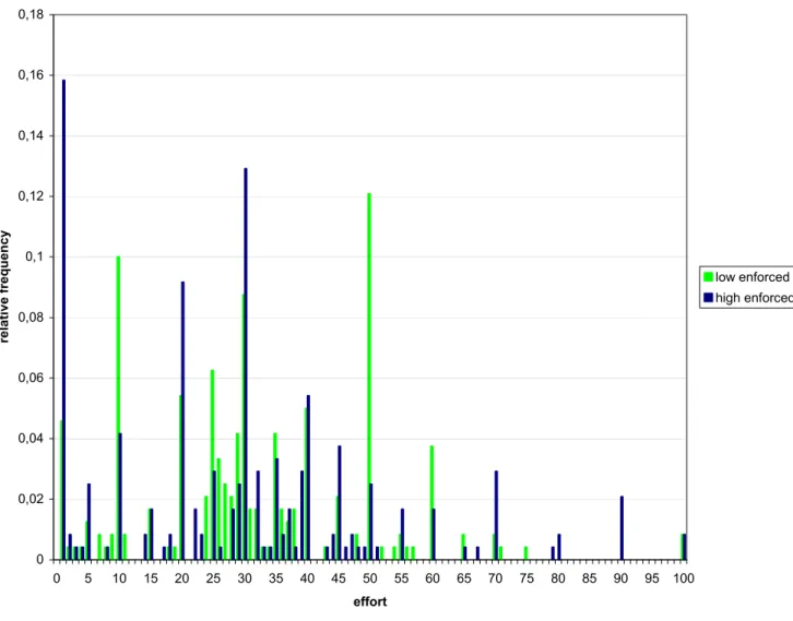
(32) 0,18. 0,16. 0,14. relative frequency. 0,12. 0,1 low enforced high enforced 0,08. 0,06. 0,04. 0,02. 0 0. 5. 10. 15. 20. 25. 30. 35. 40. 45. 50. 55. 60. 65. 70. 75. 80. 85. 90. effort. Figure 4b: Density of team effort in the ENFORCED ASYM treatment. 29. 95. 100.

(33) 100 90 80. average effort. 70 60 50 40 30 20 10 0 1 2. 3 4. 5 6. 7. 8 9 10 11 12 13 14 15 16 17 18 19 20 21 22 23 24 25 26 27 28 29 30. period effort low cost. effort high cost. eq low cost. eq high cost. opt low cost. opt high cost. Figure 5: Average team effort of low and high-cost players in the ENFORCED ASYM treatment. 30.

(34) Table 1 The parameter values Parameterization. k1. k2. p. t. SYM. 1/10. 1/10. 9. 10. ASYM. 1/10. 1/8. 7. 8. Table 2 The theoretical predictions for the second stage of the SYM and ASYM parameterization e i*. ei**. e i'. Π i*. Πi**. Π i'. 45. 25. 50. 202.5. 187.5. 250. i = 1 (low cost). 35. 20. 40. 122.5. 104. 128. i = 2 (high cost). 28. 16. 32. 98. 112. 160. Treatment SYM i = 1, 2 ASYM. e i* ei** e i' Π i* Πi** Π i'. player i’s optimal effort under private remuneration player i’s equilibrium effort (dominant strategy) under team remuneration player i’s joint profit-maximizing effort under team remuneration player i’s maximum profit under private remuneration player i’s equilibrium profit under team remuneration player i’s profit in the joint profit-maximizing solution under team remuneration. 31.

(35) Table 3 Results of the VOLUNTARY SYM treatment Private remuneration Group. # Periods. Team remuneration. Effort. Profit. % Optimal effort. # Periods. Effort. Profit. Effort diff.. SYM1. 6. 52.25. 165.01. 25.00. 24. 51.31. 237.05. 19.79. SYM2. 26. 35.71. 138.68. 1.92. 4. 50.75. 202.2. 22.50. SYM3. 30. 45.00. 202.50. 100.00. -. -. -. -. SYM4. 7. 47.50. 201.25. 50.00. 23. 62.20. 217.97. 10.74. SYM5. 6. 53.58. 157.18. 41.67. 24. 51.79. 236.3. 7.67. SYM6. 27. 51.81. 155.18. 40.74. 3. 49.00. 137.9. 58.00. SYM7. 14. 43.96. 183.15. 60.71. 16. 41.56. 205.65. 22.75. SYM8. 16. 44.69. 202.34. 93.75. 14. 35.07. 205.89. 12.71. Average. 16.50. 45.27. 174.35. 51.72. 13.50. 50.10. 220.08. 15.85. Table 4 Individual remuneration choices contingent on the previous mode of remuneration in the VOLUNTARY SYM treatment Remuneration in t-1. Choice in t. Team. Private. Team. 178. 133. Private. 30. 123. 208. 256. 32.

(36) Table 5 Results of the ENFORCED SYM treatment Group. Effort. Profit. Effort diff.. enfSYM1. 38.43. 173.74. 25.80. enfSYM2. 37.43. 201.33. 25.47. enfSYM3. 40.40. 205.35. 23.53. enfSYM4. 15.43. 112.36. 16.80. enfSYM5. 45.77. 240.13. 3.60. enfSYM6. 39.92. 214.90. 19.37. enfSYM7. 33.43. 190.50. 15.00. enfSYM8. 34.61. 195.52. 13.30. Average. 35.68. 191.73. 17.86. 33.

(37) Table 6 Results of the VOLUNTARY ASYM treatment Effort Private remuneration Group. ASYM1 ASYM2 ASYM3 ASYM4 ASYM5 ASYM6 ASYM7 ASYM8. Average. # Periods. 12 1 4 25 4 12 5 4. 8.375. Team remuneration. Low cost. High cost. (% opt.). (% opt.). 33.58. 28.00. (92). (100). 35.00. 25.00. (100). (0). 31.25. 41.75. (75). (50). 32.92. 18.40. (68). (0). 35.50. 28.00. (50). (100). 42.33. 33.83. (0). (83). 29.20. 29.60. (0). (60). 38.50. 42.50. (0). (0). 34.87. 27.22. 34. # Periods. Low cost. High cost. 18. 35.00. 32.11. 29. 31.55. 27.24. 26. 38.31. 38.73. 5. 60.00. 22.00. 26. 30.19. 30.00. 18. 45.89. 24.44. 25. 23.72. 28.28. 26. 35.62. 30.85. 21.625. 34.51. 30.14.

(38) Table 6 (continued) Results of the VOLUNTARY ASYM treatment Profit Private remuneration. Team remuneration. Group. # Periods. Low cost. High cost. # Periods. Low cost. High cost. ASYM1. 12. 120.09. 98.00. 18. 145.94. 136.84. ASYM2. 1. 122.50. 96.90. 29. 133.53. 137.46. ASYM3. 4. 116.88. 16.23. 26. 151.22. 98.88. ASYM4. 25. 119.58. 62.64. 5. -72.00. 261.66. ASYM5. 4. 112.65. 98.00. 26. 145.40. 127.51. ASYM6. 12. 90.88. 43.96. 18. 49.90. 202.23. ASYM7. 5. 107.00. 96.76. 25. 151.22. 107.79. ASYM8. 4. 116.65. 63.13. 26. 134.05. 143.87. Average. 8.375. 112.89. 68.06. 21.625. 127.26. 137.10. Table 7 Individual remuneration choices contingent on the previous mode of remuneration in the VOLUNTARY ASYM treatment: all players (low-cost, high-cost) Remuneration in t-1. Choice in t. Team. Private. 35. Team. Private. 319. 73. (157, 162). (27, 46). 15. 57. (10, 5). (38, 19).

(39) Table 8 Results of the ENFORCED ASYM treatment Group. Effort low. Effort high. Profit low. Profit high. enfASYM1. 36.40. 44.07. 159.13. 58.06. enfASYM2. 11.93. 18.80. 97.96. 62.32. enfASYM3. 31.63. 24.77. 96.22. 133.12. enfASYM4. 23.47. 37.77. 121.39. -96.16. enfASYM5. 33.90. 34.97. 157.39. 107.24. enfASYM6. 38.57. 33.40. 122.93. 145.86. enfASYM7. 43.67. 38.73. 113.27. 72.67. enfASYM8. 29.57. 2.03. 38.76. 124.75. Average. 31.14. 29.32. 113.38. 75.98. 36.

(40) Table 9 Voluntary choice of team remuneration (Random effects probits). SYM. ASYM Low cost [1]. [2]. [1]. 0.151 (0.367). 1.219* (0.725). Constant. 0.216 (0.375). 0.550 (0.577). 1st period. -0.187 (0.505). -1.225* (0.687). Last 5 periods. -0.581* (0.273). -0.037 (1.05). 0.293 (0.347). -0.244 (0.615). Partner’s effort below a strategic level. -0.976 (0.727) 1.225** (0.146). 0.999* (0.475). 0.385a **. 0.338**. 0.231a*. 82,647 240. -85.409 240. -52.606 240. Partner’s effort above a strategic level. 1.325** (0.387). 0.867* (0.293). ρa. 0.618** -195.045 480. Loglikelihood Nobs. High cost. *Significant at 5%; ** Significant at 1%; one- or two-tail tests, whenever appropriate. ( ) Standard-error. a: Likelihood ratio test.. 37.

(41) Table 10 Choice of effort level in the voluntary choice treatments (Least squares with fixed effects for individuals and periods). SYM Low cost. High cost. 47.600** (1.07). 32.286** (1.48). 29.772** (1.35). Team mode. -4.023 (3.11). 2.724 (2.87). -4.144 (2.67). Effort of the partner. 0.0771 (0.059). 0.0175 (0.0856). 0.107 (0.0589). 0.341. 0.367. 0.462. 480. 240. 240. Constant. R2 Nobs *. ASYM. Significant at 5%; ** Significant at 1%; (. ) Standard-error. Table 11 Choice of effort level in the enforced team remuneration treatment (Least squares with fixed effect for individuals and periods). SYM Low cost. High cost. Constant. 35.339** (0.7463). 26.872* (2.046). 15.954** (2.419). Effort of the partner. 0.2482** (0.0483). 0.1486* (0.0626). 0.4380** (0.0722). 0.297. 0.395. 0.563. 480. 240. 240. R2 Nobs *. ASYM. Significant at 5%; ** Significant at 1%; (. 38. ) Standard-error..

(42) APPENDIX: Instructions [VOLUNTARY ASYM]. You are participating in a decision-making experiment where you have the opportunity to earn money. How much money you earn depends on your own decisions, but may also depend on those of other participants. You will make individual decisions at your computer. From now on, please do not talk with other participants until the end of the experiment. In the experiment, you will be anonymously paired with another participant to form a group of two. The experiment consists of 30 repetitions, called periods. You will stay in the same group with the same other participant during all 30 periods. In each of the periods, you will be in the same decision situation. A period consists of two decision stages. We start by describing the second stage. In this stage, each participant has to choose an effort, which is an integer number between 0 and 100. The effort incurs a cost measured in Experimental Currency Units (ECU). The two members in each group have different effort costs. For one of the two group members, the effort cost is equal to the square of the chosen effort divided by 10, while for the other, it is equal to the square of the chosen effort divided by 8. Tables 1 and 1A below show for the two group members, respectively, the cost of each effort level between 1 and 100. Zero effort implies zero cost. At the beginning of the experiment, you will find an envelope with your personal effort cost table at your computer terminal. One of the two members in each group will find Table 1 (cost equals squared effort divided by 10), while the other will find Table 1A (cost equals squared effort divided by 8). In the first stage of each period, you have to choose between two modes of remuneration: a private remuneration mode and a joint remuneration mode. The remuneration mode will determine how you will be compensated for your effort. •. If you choose the private remuneration mode, you will be paid 7 ECU per effort unit that you individually choose in the second stage. The other group member will be paid 7 ECU per effort unit that he or she chooses in the second stage.. •. If both you and the anonymous other group member choose the joint remuneration mode, each of you will be paid based on the average effort in your group in the second stage. Each of you will be paid 8 ECU per unit of the average effort by you and the other group member.. •. If you choose the joint remuneration mode, but the anonymous other group member chooses the private remuneration mode, you will both adhere to the private remuneration mode. You will be paid 7 ECU per effort unit that you individually choose in the second stage. The other group member will be paid 7 ECU per effort unit that he or she chooses in the second stage.. 39.