1
The generalized additive model for the assessment of the direct, diffuse and global 1
solar irradiances using SEVIRI images, with application to the UAE 2
3
T.B.M.J. Ouarda1, 2*, C. Charron1, P.R. Marpu1 and F. Chebana2 4
5 1
Institute Center for Water and Environment (iWATER), Masdar Institute of Science 6
and Technology, P.O. Box 54224, Abu Dhabi, UAE 7
8 2
INRS-ETE, National Institute of Scientific Research, Quebec City (QC), G1K9A9, 9 Canada 10 11 12 *Corresponding author: 13 Email: [email protected] 14 Tel: +971 2 810 9107 15 16 17 December 2015 18
2
Abstract
19
Generalized additive models (GAMs) can model the non-linear relationship between a 20
response variable and a set of explanatory variables through smooth functions. GAM 21
is used to assess the direct, diffuse and global solar components in the United Arab 22
Emirates, a country which has a large potential for solar energy production. Six 23
thermal channels of the SEVIRI instrument onboard Meteosat Second Generation are 24
used as explanatory variables along with the solar zenith angle, solar time, day 25
number and eccentricity correction. The proposed model is fitted using reference data 26
from three ground measurement stations for the full year of 2010 and tested on two 27
other stations for the full year of 2009. The performance of the GAM model is 28
compared to the performance of the ensemble of artificial neural networks (ANN) 29
approach. Results indicate that GAM leads to improved estimates for the testing 30
sample when compared to the bagging ensemble. GAM has the advantage over ANN-31
based models that we can explicitly define the relationships between the response 32
variable and each explanatory variable through smooth functions. Attempts are made 33
to provide physical explanations of the relations between irradiance variables and 34
explanatory variables. Models in which the observations are separated as cloud-free 35
and cloudy and treated separately are evaluated along with the combined dataset. 36
Results indicate that no improvement is obtained compared to a single model fitted 37
with all observations. The performance of the GAM is also compared to the McClear 38
model, a physical based model providing estimates of irradiance in clear sky 39
conditions. 40
3
1. Introduction
41
Solar radiation reaching the earth is divided into different components. Direct 42
normal irradiance (DNI) refers to the radiation received from a straight beam of light 43
from the direction of the sun at its current position to a surface that is always normal 44
to that solar beam. Diffuse horizontal irradiance (DHI) is the radiation received by a 45
horizontal surface from radiation scattered by the atmosphere and coming from all 46
directions. Global horizontal irradiance (GHI) is the total amount of radiation received 47
on a surface parallel to the ground. Assessment of solar radiation on the earth’s 48
surface is of primary importance for many applications in solar energy. For instance, 49
the accurate assessment of DNI is needed for concentrating solar power systems or 50
other installations that track the position of the sun. To model the global tilt irradiance 51
for fixed flat plate collectors, the assessment of DNI, DHI and GHI is required [1, 2]. 52
Solar resource assessment is crucial for efficient realization of solar energy 53
applications, but is often limited by the lack of sufficient ground measurements which 54
incur high costs [3]. Infrared images acquired by satellites at different frequencies can 55
characterize earth’s emission and the atmospheric constituents, which can be used to 56
obtain estimates of solar radiation information in areas where there are no ground 57
measurements. Since satellite data are continuous in time and space, it would be 58
possible to perform solar resource assessment over the entire region. Solar maps 59
derived from satellite based methods have been proven to be more efficient than 60
interpolation of solar data from ground measurements [4]. 61
Data acquired from satellite images have been extensively used for estimation 62
of solar radiation on the earth’s surface. Several models classified as Physics-based, 63
empirical and hybrid models were proposed with a good adaptation for the regions of 64
4
interest. An example of the physics-based modeling is the model of Gautier et al. [5] 65
to estimate the GHI in North America. It was later on adapted by Cogliani et al. [6] 66
using Meteosat images to produce SOLARMET. The original Heliosat model of Cano 67
et al. [7] was used to estimate GHI, DNI and DHI over the USA. It was later adapted 68
by Perez et al. [8] for GOES images. The operational physical model of Schillings et 69
al. [3] was used to estimate DNI from Meteosat images. The Heliosat model has been 70
modified and improved through different versions [9-14]. Heliosat-4 model is being 71
currently validated [15, 16]. Another Physics-based model for cloud-free conditions is 72
the McClear model [17], which is based on look-up-tables established with the 73
radiative transfer model libRadtran [18]. 74
On the other hand, data-driven statistical approaches have also been frequently 75
used to perform solar radiation assessment. Artificial neural networks (ANN) have 76
been used successfully in a wide range of fields (See for instance [19-21]). They have 77
been adapted for solar resources assessment in a number of studies [22-28]. In these 78
studies, location dependent parameters and meteorological parameters were used as 79
inputs to model solar irradiance components. ANNs with an ensemble approach, 80
which provide better generalization compared to a single ANN [29, 30], were used in 81
Eissa et al. [23] to retrieve irradiance components over the UAE. A simple bagging-82
like approach was used to develop the ensemble models. Alobaidi et al. [22] further 83
improved on this model, by introducing a novel ensemble framework which 84
significantly improved the results compared to the results obtained in the previous 85
studies. The model employs a two-stage resampling process to build ensemble 86
architectures for non-linear regression. Though the model performs well, it involves 87
an ensemble of ensembles framework resulting in high computation load apart from 88
the number of computationally expensive optimization steps while training the 89
5
architecture. Another biggest drawback of ANN type models is that the relations 90
between the inputs and outputs cannot be explicitly presented. 91
In this work, we propose to use the generalized additive model (GAM), which 92
is an extension of the generalized linear model (GLM) which uses non-parametric 93
smooth functions to relate explanatory variables to the response variable. This flexible 94
method represents an interesting approach to model the complex relation between 95
irradiance and explanatory variables. GAMs have been applied widely in 96
environmental studies [31-35], and in public health and epidemiological studies [36-97
41]. However, GAMs have never been used for solar irradiance assessment. An 98
advantage of GAM over ANN is that the relationship between each predictor and the 99
response variable is made explicit through a set of smooth functions. 100
The United Arab Emirates (UAE) presents a high potential for solar energy 101
development due to the long day light period and the marginal amount of cloud cover. 102
Recently, Eissa et al. [23, 42] and Alobaidi et al. [22] developed models to accurately 103
estimate irradiance components over the UAE territory in which they used images of 104
the earth’s surface acquired by the Spinning Enhanced Visible and Infrared Imager 105
(SEVIRI) onboard Meteosat Second Generation (MSG) satellite. 106
The aim of the present paper is to use GAM for the assessment of the 107
irradiance components DHI, DNI and GHI using SEVIRI satellite images. Following 108
previous work, six SEVIRI thermal channels along with the solar zenith angle (Z), 109
solar time (Time), day number (Day) and eccentricity correction (ε) are used as 110
explanatory variables in the model. 111
In Eissa et al. [23], DHI was directly estimated with the ANN but DNI was 112
deduced from the ANN estimated optical depth (δ) and GHI was deduced from DNI 113
6
and DHI estimates. In the present study, we propose also to estimate directly the DNI 114
and GHI with GAM. In Eissa et al. [23] and Alobaidi et al. [22], an algorithm was 115
used to separate the training and the testing dataset as cloud-free and cloudy sub-116
datasets. ANN models were then trained and tested separately on the two sky 117
condition samples. While this approach is also considered in the present work, we 118
additionally propose to develop a global model to the all sky training dataset and to 119
validate it on the cloud-free, cloudy and all sky testing datasets. GAM allows 120
explicitly defining the relationship between the response variable and each 121
explanatory variable through smoothing functions. Attempts to find physical 122
interpretations of the shape of these curves are made in the present work. 123
A comparison is also made with the McClear model, a physical based model 124
providing estimates of irradiance in clear sky conditions. The results of McClear 125
model are available through a web service at the website of the MACC project 126
(Monitoring Atmospheric Composition and Climate project) (http://www.gmes-127
atmosphere.eu). Estimates could be obtained by just providing the latitude, longitude 128
and the altitude (optional) of the target site, and the period of interest. 129
130
2. Data
131Ground measurements for DHI, DNI and GHI consist of 10 min resolution 132
data available at 5 stations over the UAE. At each station, data are collected using a 133
Rotating Shadowband Pyranometer (RSP). GHI is measured by the pyranometer 134
when the shadowband is stationary. The shadowband makes a full rotation around the 135
pyranometer. DHI is given by the lowest measured irradiance since at that moment 136
DNI is completely blocked by the shadowband. DNI is deduced from GHI and DHI 137
7
measured with the RSP. In the following, ground measured DNI refers to DNI that is 138
estimated from ground measured GHI and DHI. To match the 15 min resolution of the 139
satellite data, successive ground measured data were interpolated. Data are available 140
for the full year 2009 at the stations of Masdar City, Al Aradh and Madinat Zayed, 141
and for the full year 2010 at all stations. Fig. 1 presents the spatial distribution of the 142
stations across the UAE. 143
Satellite images of the SEVIRI optical imager onboard MSG satellite were 144
used in the present study. They provide continuous images of the earth in 12 spectral 145
channels with a temporal resolution of 15 min and a spatial resolution of 3 km. 146
Images from 6 thermal channels, T04 (3.9 μm), T05 (6.2 μm), T06 (7.3 μm), T07 (8.7 147
μm), T09 (10.8 μm) and T10 (12.0 μm) were collected and converted into brightness 148
temperature. For each station, 3-by-3 pixels, with the station located in the center 149
pixel, were extracted from satellite data. The other variables, solar zenith angle (Z), 150
Time, Day and eccentricity correction ε were computed for each pixel. The choice of 151
the selected thermal channels is justified in Eissa et al. (2013) by their sensitivity to 152
the different constituents of the atmosphere: channel T05 and T06 are known to be 153
affected by water vapor and T07, T08 and T09 are frequently used for dust detection. 154
T04 was also selected in Eissa et al. (2013) because it had improved their model 155
accuracy. 156
The dataset is divided into training and testing datasets. The model is 157
developed using the training dataset and tested using the testing dataset. The training 158
dataset includes data from the stations of Masdar City, East of Jebel Hafeet and Al 159
Wagan for the full year 2010. The testing dataset includes data from the stations of Al 160
Aradh and Madinat Zayed for the full year 2009. The training and testing datasets are 161
8
further divided respectively into cloud-free and cloudy datasets. For this, a cloud 162
mask was applied in which each pixel was classified as cloud-free or cloudy. The thin 163
cirrus test [43], employing the T09 and T10 channels of SEVIRI, was used as a cloud 164
mask following [23]. In all, the cloud-free and cloudy training datasets contain 29193 165
and 7086 observations respectively, and the cloud-free and cloudy testing datasets 166
contain 16864 and 2856 observations respectively. 167
168
3. Methodology
1693.1 Generalized Additive Model
170
GLMs [44] generalize the linear model with a response distribution other than 171
normal and a link function relating the linear predictor with the expectation of the 172
response variable. Let us define Y, a random variable called response variable, and X, 173
a matrix whose columns are a set of r explanatory variables X1, X2,…, Xr. The GLM 174
model is defined by: 175 1 [ ( | )] r j j j g E Y X
X , (1) 176where g is the link function and j and α are unknown parameters. With GLM, the 177
distribution of Y is generalized to have any distribution within the exponential family. 178
The role of the link function is used to transform Y to a scale where the model is 179
linear. 180
The GAM model [45] is an extension of the GLM in which the linear predictor 181
is replaced by a set of non-parametric functions of the explanatory variables. GAM 182
can then be expressed by: 183
9 1 [ ( | )] ( ) r j j j g E Y f X
X , (2) 184where f j are smooth functions of X j. This model is more flexible by allowing non-185
linear relations between the response variable and the explanatory variables through 186
the smooth functions. Because of the additive structure of GAM, the effect of each 187
explanatory variable on Y can be easily interpreted. A smooth function can be 188
represented by a linear combination of basis functions: 189 1 ( ) ( ) j q j j ji ji j i f x b x
, (3) 190where bji(xj) is the ith basis function of the jth explanatory variable evaluated at 191
j
x , qj is the number of basis functions for the jth explanatory variable and ji are
192
unknown parameters. 193
Given a basis function, we define a model matrix Zj for each smooth 194
function where the columns of Zj are the basis functions evaluated at the values of 195
the jth explanatory variable. Eq. (2) can be rewritten as a GLM in a matrix form as: 196
(E( ))
g y Zθ, (4)
197
where y is a vector of observed values of the response variable Y, Z is a matrix 198
including all the model matrix Zj and θ is a vector including all the smooth 199
coefficient vectors θj. Parameters θ could be estimated by the maximum likelihood 200
method, but if qj is large enough, the model will generally overfit the data. For that
201
reason, GAM is usually estimated by penalized likelihood maximization. The penalty 202
is typically a measure of the wiggliness of the smooth functions and is given by: 203
10
T
jSj j
θ θ for the jth smooth function where Sj is a matrix of known coefficients. The
204
penalized likelihood maximization objective is then given by: 205 T 1 ( ) ( ) 2 p j j j j j l θ l θ
θ S θ . (5) 206where l θ( ) is the likelihood of θ and j are the smoothing parameters which 207
control the degree of smoothness of the model. For given values of the parameters j 208
, the GAM penalized likelihood can be maximized by penalized iterative re-weighted 209
least squares (P-IRLS) to estimate θ (see [46]). However, j should be estimated by 210
an iterative method like Newton’s method [46]. For each trial of j, the P-IRLS is 211
iterated to convergence. In this study, j are optimized by minimizing the 212
generalized cross validation score (GCV), which is based on the leave-one-out 213
method. This method ends up being computationally less expensive as it can be 214
shown that the GCV score equals: 215
2 2 ˆ tr( ) g n n y Z A θ , (6) 216where AZ ZZ( Z)1Z is the influence matrix. In this study, all GAM model T
217
parameters are estimated with the R package mgcv [46]. 218
The smooth functions used in this study are cubic regression splines. Cubic 219
splines are constructed with piecewise cubic polynomials joined together at points 220
called knots. The definition of the cubic smoothing spline basis arises from the 221
solution of the following optimization problem [47]: Among all functions f x( ), with 222
11
two continuous derivatives, find one that minimizes the penalized residual sum of 223 squares: 224 2 2 1 { ( )} λ ( ) n b i i a i y f x f x dx
, (7) 225where y y1, 2, ,y is a set of observed values of the response variable and n 226
1, 2, , n
x x x a set of observed values of an explanatory variable, λ is the smoothing 227
parameter, and ax1x2 xn b. The first term of (7) measures the degree of 228
fit of the function to the data, while the second term adds a penalty for the curvature 229
of the function, and the smoothing parameter controls the degree of penalty given for 230
the curvature in the function. With regression splines, the numbers of knots can be 231
considerably reduced, and the position of the knots needs to be chosen. In fact, with 232
cubic penalized splines, the exact location of the knots and their numbers are not as 233
important as the smoothing parameters. In this study, the positions of the knots will be 234
evenly spaced along the dimension of each explanatory variable. 235
3.2 Model configurations
236
For the GAM models of this study, the identity link function and the Gaussian 237
error with mean zero and a constant variance 2
are assumed. In each model, 238
residuals obtained are checked for any trends in the variance and for normality to 239
confirm the model assumptions. In Eissa et al. [23], DHI was estimated directly with 240
the ANN trained with ground measured DHI. The model for the GAM estimated DHI 241
is given by the following expression: 242 1 DHI ( ) r j j j f X
, (8) 24312
where X j is the jth explanatory variable, r is the number of explanatory variable
244
included in the model and is the intercept. 245
DNI estimations in Eissa et al. [23] were deduced from the ANN estimated δ. 246
DNI estimations were then computed using the Beer-Bouguer-Lambert law which 247
relates δ to DNI by the following equation: 248
0
DNII exp(m), (9)
249
where I is the solar constant with an approximate value of 1367 W/m2, and m is the 0 250
air mass. The values of δ were computed from ground measured DNI. Parameters m 251
and ε can be easily computed for any location on a given day by knowing Z. For 252
the estimation of δ with GAM, the following model is used: 253 1 log( ) ( ) r j j j f X
. (10) 254The logarithmic transformation of δ in (10) is used to meet the model assumptions. 255
Fig. 2 presents the residuals against the fitted values for the models with and without a 256
logarithmic transformation. Fig. 2b clearly improves the residual constant variance 257
assumption. In this study, we also propose to estimate DNI directly with GAM fitted 258
on ground measured DNI. Estimated DNI is then denoted by DNID and the following 259
model similar to that of DHI, is used: 260 D 1 DNI ( ) r j j j f X
. (11) 261The GHI is deduced from the estimated DHI and DNI using the following 262
relation: 263
13
GHIDNI cosZ DHI. (12)
264
In this study, we also propose to estimate GHI directly with GAM fitted on ground 265
measured GHI. Estimated GHI is then denoted by GHID and the following model is 266 used: 267 D 1 GHI ( ) r j j j f X
. (13) 268 269 3.3 Validation method 270For comparison with the results of Eissa et al. [23] and Alobaidi et al. [22], the 271
same validation method is used in the present study. On the 5 ground stations in the 272
UAE, the data from 3 stations for the full year 2010 are used for fitting the model and 273
the data from the 2 remaining stations for the full year 2009 are used for testing the 274
model. With this approach, the model is trained and tested on completely independent 275
conditions with different locations and a different year. 276
The performances are evaluated in terms of the root mean square error 277
(RMSE), mean bias error (MBE), relative root mean square error (rRMSE) and 278
relative mean bias error (rMBE). The rRMSE and rMBE are defined here by: 279
1 1 100 ˆ n i i i rRMSE y y n y
, (14) 280
1 1 100 ˆ n i i i rMBE y y n y
(15) 28114
where y is the measured irradiance, ˆi y is the estimated irradiance and i y is the 282
mean of the measured irradiance. 283
284
4. Results
2854.1. Models trained and tested on the cloud–free and cloudy sky datasets
286
This subsection presents the results of the estimation of irradiance variables 287
with GAM. Two separate models for each irradiance variable were fitted on the 288
cloud-free and cloudy training datasets with all the explanatory variables included. 289
Finally, each model was validated with either the cloud-free or the cloudy testing 290
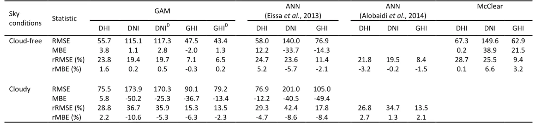
dataset. Table 1 presents the results obtained for the irradiance variables in terms of 291
RMSE, MBE, rRMSE, and rMBE for cloud-free and cloudy conditions, and for both 292
GAM and ANN models. 293
The comparison of the relative statistics obtained with GAM indicates that 294
best estimations are obtained for GHI and GHID in both sky conditions. The rRMSEs 295
reach their lowest values for GHI and GHID (7.1% and 6.5% for cloud-free conditions 296
and 15.3% and 13.5% for cloudy conditions respectively). In cloud-free conditions, 297
the worst estimations are obtained for DHI with an rRMSE of 23.8%. In the cloudy 298
case, the worst estimations are obtained for DNI and DNID with rRMSEs equal to 299
36.7% and 35.9% respectively. When comparing results for cloud-free and cloudy 300
conditions, the worst estimations are systematically obtained for cloudy conditions. 301
The rRMSE and rMBE values are significantly higher for cloudy conditions for most 302
irradiance variables compared to cloud-free conditions. 303
15
Results for DNID and GHID, directly estimated with GAM, are compared with 304
results for DNI and GHI. In cloud-free conditions, GHID results are slightly better 305
than GHI, while DNI results are slightly better than DNID. In cloudy conditions, 306
absolute and relative RMSEs are improved slightly with directly estimated DNI and 307
GHI. More important improvements are observed for absolute and relative MBEs: For 308
instance, absolute MBEs obtained for DNI and DNID in cloudy conditions are -50.2 309
and -25.3 W/m2 respectively. For GHI and GHID, they are -36.7 and -13.4 W/m2 310
respectively. 311
For comparison purposes, results obtained in Eissa et al. [23] and Alobaidi et 312
al. [22] with the ANN approach using the same case study and validation procedure 313
are presented in Table 1. Comparison of GAM and Bagging ANN results of Eissa et 314
al. [23] shows that significant improvements are generally obtained with GAM for 315
DNI, DNID, GHI and GHID with respect to absolute and relative RMSE and MBE for 316
both sky conditions. For instance, in the case of cloud-free conditions, the RMSE for 317
DNI is 140.0 W/m2 with ANN compared to 115.1 W/m2 with GAM. For DHI, 318
RMSEs are relatively similar in both sky conditions but MBEs are significantly better 319
for GAM in both sky conditions. Overall, the results indicate a clear advantage of 320
GAM over ensemble ANN model of Eissa et al. [23]. 321
The results of Alobaidi et al. [22] are comparable for the cloud-free conditions 322
and are slightly better for the cloudy conditions. For the cloud-free conditions, the 323
RMSE of the proposed GAM model is slightly higher for DHI, but the results of 324
GAM model have lower MBE. The DNI results are very similar. The GAM model 325
however produces better estimates of the GHI for cloud free conditions which implies 326
that the errors in DHI and DNI cancel each other. 327
16
4.2. A single model trained on all sky dataset and tested on cloud–free, cloudy
328
and all sky datasets
329
In Eissa et al. [23] and Alobaidi et al. [22], two different ANN ensemble 330
models were trained and tested separately for cloud-free and cloudy datasets. The 331
impact of using separate datasets based on sky conditions is evaluated here. For that, a 332
global model was fitted to the all sky conditions dataset and tested separately on the 333
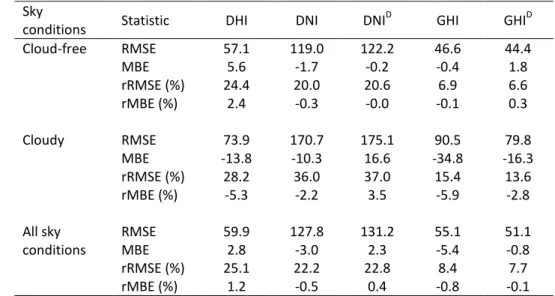
cloud-free, cloudy and all sky testing datasets. Results obtained with the global model 334
are presented in Table 2. In the following, they are compared to the results of Table 1. 335
For the cloud-free case, RMSEs are in most cases slightly higher with the global 336
model and MBEs equivalent for both approaches. For the cloudy case, no general 337
conclusion can be made concerning RMSEs and MBEs. However, MBEs are 338
significantly reduced for DNI and DNID with the global model. For the all sky 339
conditions case, relative statistics represent a tradeoff between results when tested on 340
the cloud-free testing dataset and when tested on the cloudy testing dataset. This 341
reflects the fact that both sky conditions testing datasets are mixed together. These 342
overall results show that using separate models trained on cloud-free and cloudy 343
conditions do not have a significant positive impact on the performances. 344
Fig. 3 presents the density scatter plots of estimated variables versus ground 345
measured variables. For DHI, a downward trend in residuals is observed and a 346
positive bias is visible in the zone with the highest density. DNI and DNID present 347
similar scatter plots. A downward trend in residuals is also observed for these 348
variables. Residuals in the scatter plot of for GHI and GHID are similar. They are 349
evenly distributed around the line representing zero bias and no trend is observed. 350
17
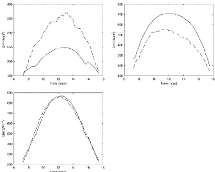
Mean ground measured DHI, DNI and GHI were computed for separate cloud-351
free and cloudy conditions. Fig. 4 presents the mean ground measured DHI, DNI and 352
GHI as a function of time for the training dataset. Cloud-free and cloudy conditions 353
were computed separately. For DHI, the received irradiance is superior for cloudy 354
conditions. For DNI, the inverse occurs where the irradiance received is superior for 355
cloud-free conditions. For GHI, both curves confound each other. These curves are 356
explained by the fact that under cloudy sky conditions, the scatter irradiance is 357
increased, resulting in an increased DHI and a reduced DNI. However, the total 358
irradiance received is not affected by sky conditions as GHI is equal for both 359
conditions. These results advocate the use a single model for both sky conditions for 360
GHI. 361
4.3 Interpretation of smooth functions
362
In GAM, the sum of the smooth functions of one or more explanatory 363
variables and the intercept give a function of the response variable (See (2)). Each 364
smooth function then represents the effect on the response variable of one predictor in 365
relation with the effect of the other predictors. Smooth functions are graphically 366
presented here and attempts to provide physical explanations are made. The global 367
model fitted on the all sky conditions training dataset is used here for illustration as no 368
important improvement was obtained by using two separate models for both sky 369
conditions as shown in the last subsection. 370
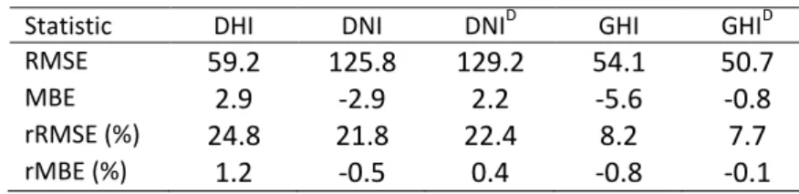
Attempts to obtain simpler models were carried out through stepwise 371
regression methods. However, in most cases, the best model ends up being the model 372
with all variables. Nevertheless, with GAM, it is hypothesized that the inclusion of ε 373
is unnecessary. Indeed, ε is computed at each location with a formula that depends 374
18
only on day number, which is already included as an explanatory variable in the 375
model. Table 3 presents the results obtained for the estimation of radiation variables 376
with models using all explanatory variables except ε. The results obtained with and 377
without ε are very similar and show that ε is redundant. 378
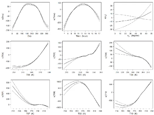
The smooth functions of each explanatory variable are represented in Figs. 5-7 379
for DHI, DNID and GHID respectively using the model without ε and fitted on the all 380
sky conditions training dataset. The dotted line represents the 5% confidence interval. 381
To help interpreting the smooth functions, Figs. 8-10 present the scatter plots of 382
measured DHI, DNI and GHI versus each explanatory variable respectively for the all 383
sky conditions training dataset. 384
The smooth function of DHI versus Day increases with Day until summer then 385
decreases until the end of the year. The scatter plot of DHI with Day in Fig. 8 shows a 386
similar relation. For DNID and GHID, an inverse relation in the smooth functions is 387
observed where the irradiance reaches its minimum during summer. The scatter plot 388
of DNI with Day in Fig. 9 reveals a similar relation. This result is counterintuitive 389
because irradiance is expected to increase during summer. A possible explanation 390
could be the significantly higher air humidity during summer and/or more dust 391
scattering the solar radiation during the summer season. 392
The smooth function of DHI versus Time increases with time to reach a 393
maximum at around noon and decreases afterwards. Because time is related to the sun 394
height and therefore to irradiance intensity, it is expected to observe a similar shape of 395
smooth curve for every irradiance variable. However, for DNID and GHID, an inverse 396
relation is observed where the minimum irradiance is reached at around noon. This 397
behavior is explained by the fact that the explanatory variable Z, included in the 398
19
model, also explains the sun position. In the case of DHI, the smooth function of Z 399
is strictly increasing. In this case, the time explains the sun position and Z explains a 400
complementary portion of the total variance. In the case of DNID and GHID, Z rather 401
explains the sun position as the smooth functions are strictly decreasing with Z. 402
The interpretation of the smooth functions of the predictors related to thermal 403
channels is difficult because of their number and the fact that they are not 404
independent. In all cases, a change in the slope of the curve occurs in mid-405
temperatures. Confidence intervals are larger for low temperatures and decrease to 406
become very small with increasing temperatures. This is explained by the fact that 407
there are fewer observations for small temperatures as seen in the scatter plots of Figs. 408
8-10. 409
The analysis of the smooth curves seems to indicate that the seasonal pattern 410
may be caused by the solar scattering by airborne particles. To further study this 411
hypothesis we quantified the aerosol particle content over the UAE, using data from 412
the AERONET map (AErosol RObotic NETwork), a ground-based aerosol 413
monitoring network initiated by NASA [48]. The dataset includes the aerosol optical 414
thickness (AOT) for different wavelengths and the total water vapor in the column. 415
Fig. 11 presents the mean daily aerosol optical thickness (AOD) at the wavelength of 416
500 nm and the mean daily water vapor at the Abu Dhabi station (24.44 ºN, 54.62 ºE). 417
This figure shows an important seasonality in the dust and the water vapor peaking 418
during summer. 419
A strong seasonality is observed in both water vapor and aerosol optical 420
thickness. It is therefore important to verify whether this seasonal behavior propagates 421
20
also into the performance statistics. For this purpose, the year of the testing sample 422
was divided in four seasons of three months and the performance statistics were 423
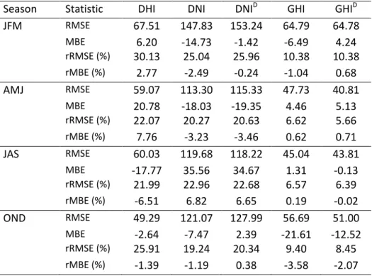
computed for each season. Table 4 presents the performances for each season with the 424
models without ε, fitted and tested on the all sky conditions training and testing 425
datasets (i.e., the same models used in Table 3). The results of Table 4 show that 426
biases are in general higher during the summer (AMJ and JAS) and RMSEs are higher 427
during the winter season of JFM. The high bias values associated to the summer 428
season can be explained by the scattering by aerosol constituents. It is also observed 429
that the biases of DHI are generally of opposite sign than DNID and DNI. GHI biases 430
are generally very small due to the canceling effect of the DHI and DNI biases. 431
In the second stage, the number of thermal channels was reduced in order to 432
ease the physical interpretation of the smooth functions related to the thermal 433
channels. In this way, only three thermal channels, T04, T05 and T09, in addition to 434
the other variables were included in the models. T05 and T09 were chosen to 435
represent the water vapor and dust constituents of the atmosphere and T04 was 436
selected because it was shown to be an important channel in the models. Smooth 437
functions obtained for each explanatory variable are presented in Figs. 12-14 for 438
variables DHI, DNID and GHID. Performances obtained with this configuration are 439
shown in Table 5. Because the number of explanatory variables has been reduced, 440
most performance indicators decreased. However, RMSE values are similar for GHI 441
and GHID and absolute and relative MBE values for DNI have improved for the 442
model with fewer explanatory variables. 443
Smooth functions of variables Day, Time and Z have similar relationships 444
with response variables than those obtained with the model with more variables. 445
21
There is an exception in the case of DHI for Z where the smooth function is now 446
strictly decreasing. For the thermal channels, most observations occur after a certain 447
threshold temperature which is channel dependent. This can be clearly seen in the 448
scatter plots. Consequently, a change in slope occurs generally around this threshold 449
temperature in the smooth functions of thermal channels. As the number of 450
observations is negligible for the temperatures below the threshold, the analysis is 451
restricted on temperatures higher than this threshold. For DHI, T09 is the most 452
important thermal channel. Its smooth function has a strong negative slope. On the 453
other hand, the smooth function for T04 increases continuously. The smooth function 454
of T05 increases continuously with a light slope. The scatter plots of Fig. 8 reveal that 455
DHI has a positive relation with temperature for T04. For DNID, T09 is the most 456
important thermal channel. Its smooth function increases constantly with a strong 457
slope. The smooth function of T04 decreases continuously with a strong slope for 458
high temperatures (Fig. 13). The smooth function of T05 has a light decreasing slope. 459
A strong positive relation of DNI with temperature for T09 is also observed in Fig. 9 460
while being less important for T04. For GHI, the smooth functions of T04 and T09 461
are both strictly increasing (Fig. 14). Strong positive relations are also observed in the 462
scatter plots of thermal channels T04 and T09 in Fig. 10. The smooth function of T05 463
has a slope of about zero and is thus not very important. 464
The thermal channels T05 and T09 were chosen to represent respectively 465
water vapor and dust in the atmosphere. We aim to evaluate to which extent these 466
thermal channels capture the seasonality of the airborne constituents. For this, the 467
individual thermal channel components of the linear predictor are displayed as a 468
function of the day of the year. The simplified models DHI and DNID fitted on the all 469
sky conditions dataset are considered. Fig. 15 presents the mean daily predicted DHI 470
22
and DNI as a function of the day. It can be observed that the curves for T04 follow the 471
seasonal evolution of the ground temperature with a peak during summer. For T05, a 472
strong attenuation due to water vapor is observed where no noticeable seasonality can 473
be observed. For T09, the same seasonal pattern than T04 is notice but with a small 474
attenuation during summer due to dust. Fig. 16 presents the daily mean ground-475
measured thermal channels T04, T05 and T09 as a function of the day for the all sky 476
conditions training dataset. 477
4.5 Comparison with McClear
478
Using the web service for McClear, estimates of irradiances were obtained at 479
the two stations included in the testing sample during the same time period. 480
Performance statistics computed for the cloud-free condition testing sample are added 481
in Table 1. Fig. 17 presents the density scatter plots of estimated variables with 482
McClear versus ground measured variables. Scatter plots are rather similar to GAM. 483
Same trends are observed in the residuals. One small difference that can be observed 484
is that more observations of DHI are underestimated with McClear for very high 485
irradiances. There is also more positive bias with McClear for very low DNI. 486
Performances presented in Table 1 show that McClear, compared to GAM, has higher 487
RMSEs for all variables and higher biases for DNI and GHI. In Eissa et al. [49], the 488
McClear model was validated for the same stations as in the present study and better 489
performances were obtained. This can be explained by the fact that the two 490
publications used different methods to discriminate the cloud-free samples from the 491
cloudy samples. Indeed, the algorithm of Long and Ackerman [50] was used in Eissa 492
et al. [49] instead of the thin cirrus method used in the present work and in Eissa et al. 493
[49]. The application of the Long and Ackerman method has resulted in a much lower 494
proportion of retained cloud-free instants where only 65% of the data was considered 495
23
cloud-free compared to 85% in the case of the present work. The algorithm of Long 496
and Ackerman is more restrictive in its discrimination and might have removed some 497
instants that were in fact cloudy. 498
499
5. Conclusions
500In this study, GAM was used to estimate the irradiance components DHI, DNI 501
and GHI in the UAE. Ground irradiance measurements were available at 5 stations 502
over the UAE. The data from three stations for the full year of 2010 were used to fit 503
the model and the data of the two remaining stations for the full year of 2009 were 504
used for the validation. In this way, the model was trained and tested in completely 505
independent temporal and spatial conditions. For the purpose of estimating irradiance 506
throughout the UAE, six SEVIRI thermal channels were used along with other 507
variables including the solar zenith angle Z, Day, Time and the eccentricity 508
correction ε. These variables can be calculated for any location over the UAE. 509
Results were compared with those obtained with an ANN ensemble approach 510
in Eissa et al. [23] and Alobaidi et al. [22] where the same database and validation 511
procedure were used. Results indicate clearly that GAM leads to an improved 512
estimation when compared with the bagging ensemble, and is similar or better for 513
cloud-free conditions and slightly lower for cloudy conditions compared to the two-514
stage ensemble architecture proposed in Alobaidi et al. [22]. However, the simplicity 515
of the GAM models and their ability to provide explicit expressions unlike the ANN 516
ensemble is a clear advantage. 517
24
In Eissa et al. [23], the training and testing datasets were separated into cloud-518
free and cloudy sub-datasets and models were fitted and tested separately for these 519
two datasets. The same approach was used in Alobaidi et al. [22] as well. The 520
obtained estimations were weaker in the case of cloudy conditions. In the present 521
study, a single model was also fitted using the training data for all sky conditions and 522
was tested on the cloud-free and cloudy testing datasets. Results have shown that 523
similar performances were obtained for both sky conditions with the global model. 524
This suggests that using two different models is not necessary. 525
As mentioned before, the advantage of the GAM approach over the ANN 526
approach is that relations between irradiance variables and explanatory variables can 527
be defined explicitly. The smoothing curves for each explanatory variable were 528
graphically represented and analyzed to provide physical explanations to the modeled 529
relations. 530
It is proposed in future work to add more variables such as relative humidity 531
as explanatory covariates. Relative humidity has a high variability throughout the 532
year, with large values during the summer. Its inclusion as covariate may help explain 533
an additional percentage of the variance, especially in the summer season. The 534
development of specific summer and winter models based on a rational definition of 535
the seasons (see for instance [51]) should also lead to improved models. The usage of 536
coarse resolution aerosol maps normally used in the physics based approaches can 537
also be integrated into the proposed framework. Future efforts can also focus on 538
testing more advanced basis functions in the GAM model. 539
540
Acknowledgment
54125
The authors thank the Editor, Dr. Qian Du, the associate editor and the two anonymous
542
reviewers for their judicious comments. The authors also thank the staff responsible for
543
maintaining the AERONET stations in the UAE.
544 545
Nomenclature
546DNI direct normal irradiance (W/m2) 547
DHI diffuse horizontal irradiance (W/m2) 548
GHI global horizontal irradiance (W/m2) 549
Z
solar zenith angle (degrees) 550
eccentricity correction 551
total optical depth of the atmosphere 552 0 I solar constant (1367 W/m2) 553 m air mass 554
T04 SEVIRI T04 channel (3.9 μm) observed brightness temperature (K) 555
T05 SEVIRI T05 channel (6.2 μm) observed brightness temperature (K) 556
T06 SEVIRI T06 channel (7.3 μm) observed brightness temperature (K) 557
T07 SEVIRI T07 channel (8.7 μm) observed brightness temperature (K) 558
T09 SEVIRI T08 channel (10.8 μm) observed brightness temperature (K) 559
T10 SEVIRI T10 channel (12.0 μm) observed brightness temperature (K) 560
ANN artificial neural network 561
GAM generalized additive model 562
GLM generalized linear model 563
RMSE root mean square error 564
MBE mean bias error 565
rRMSE relative RMSE (%) 566
rMBE relative MBE (%) 567
X matrix of explanatory or independent variables 568
26
Z model matrix for the basis functions 569
A influence matrix
570
Y response or dependent random variable 571
X explanatory or independent random variable 572
y vector of observed values of Y 573
g the link function in GAM and GLM 574
unknown parameters of the linear model 575
θ vector of unknown parameters of the basis functions 576
f smooth functions
577
b spline basis functions 578
λ smoothing parameter 579
27
References
580
581
[1] C. A. Gueymard, "Direct and indirect uncertainties in the prediction of tilted 582
irradiance for solar engineering applications," Solar Energy, vol. 83, pp. 432-583
444, 2009. 584
[2] B. Y. H. Liu and R. C. Jordan, "The long-term average performance of flat-585
plate solar-energy collectors: With design data for the U.S., its outlying 586
possessions and Canada," Solar Energy, vol. 7, pp. 53-74, 1963. 587
[3] C. Schillings, H. Mannstein, and R. Meyer, "Operational method for deriving 588
high resolution direct normal irradiance from satellite data," Solar Energy, vol. 589
76, pp. 475-484, 2004. 590
[4] A. Zelenka, R. Perez, R. Seals, and D. Renné, "Effective Accuracy of 591
Satellite-Derived Hourly Irradiances," Theoretical and Applied Climatology, 592
vol. 62, pp. 199-207, 1999/04/01 1999. 593
[5] C. Gautier, G. Diak, and S. Masse, "A Simple Physical Model to Estimate 594
Incident Solar Radiation at the Surface from GOES Satellite Data," Journal of 595
Applied Meteorology, vol. 19, pp. 1005-1012, 1980. 596
[6] E. Cogliani, P. Ricchiazzi, and A. Maccari, "Physical model SOLARMET for 597
determinating total and direct solar radiation by meteosat satellite images," 598
Solar Energy, vol. 81, pp. 791-798, 2007. 599
[7] D. Cano, J. M. Monget, M. Albuisson, H. Guillard, N. Regas, and L. Wald, "A 600
method for the determination of the global solar radiation from meteorological 601
satellite data," Solar Energy, vol. 37, pp. 31-39, 1986. 602
[8] R. Perez, P. Ineichen, K. Moore, M. Kmiecik, C. Chain, R. George, and F. 603
Vignola, "A new operational model for satellite-derived irradiances: 604
description and validation," Solar Energy, vol. 73, pp. 307-317, 2002. 605
[9] H. G. Beyer, C. Costanzo, and D. Heinemann, "Modifications of the Heliosat 606
procedure for irradiance estimates from satellite images," Solar Energy, vol. 607
56, pp. 207-212, 1996. 608
[10] A. Hammer, D. Heinemann, C. Hoyer, R. Kuhlemann, E. Lorenz, R. Müller, 609
and H. G. Beyer, "Solar energy assessment using remote sensing 610
technologies," Remote Sensing of Environment, vol. 86, pp. 423-432, 2003. 611
[11] R. W. Mueller, K. F. Dagestad, P. Ineichen, M. Schroedter-Homscheidt, S. 612
Cros, D. Dumortier, R. Kuhlemann, J. A. Olseth, G. Piernavieja, C. Reise, L. 613
Wald, and D. Heinemann, "Rethinking satellite-based solar irradiance 614
modelling: The SOLIS clear-sky module," Remote Sensing of Environment, 615
vol. 91, pp. 160-174, 2004. 616
[12] J. Polo, L. Martín, and M. Cony, "Revision of ground albedo estimation in 617
Heliosat scheme for deriving solar radiation from SEVIRI HRV channel of 618
Meteosat satellite," Solar Energy, vol. 86, pp. 275-282, 2012. 619
[13] C. Rigollier, M. Lefèvre, and L. Wald, "The method Heliosat-2 for deriving 620
shortwave solar radiation from satellite images," Solar Energy, vol. 77, pp. 621
159-169, 2004. 622
[14] M. Schroedter-Homscheidt, J. Betcke, G. Gesell, D. Heinemann, and T. 623
Holzer-Popp, "Energy-Specific Solar Radiation Data from MSG: Current 624
Status of the HELIOSAT-3 Project," in Second MSG RAO Workshop, 2004, p. 625
131. 626
28
[15] Z. Qu, A. Oumbe, P. Blanc, M. Lefevre, L. Wald, M. S. Homscheidt, G. 627
Gesell, and L. Klueser, "Assessment of Heliosat-4 surface solar irradiance 628
derived on the basis of SEVIRI-APOLLO cloud products," in 2012 629
EUMETSAT Meteorological Satellite Conference, 2012, pp. s2-06. 630
[16] Z. Qu, A. Oumbe, P. Blanc, M. Lefevre, L. Wald, M. Schroedter-Homscheidt, 631
and G. Gesell, "A new method for assessing surface solar irradiance: Heliosat-632
4," in EGU General Assembly Conference Abstracts, 2012, p. 10228. 633
[17] M. Lefèvre, A. Oumbe, P. Blanc, B. Espinar, B. Gschwind, Z. Qu, L. Wald, 634
M. Schroedter-Homscheidt, C. Hoyer-Klick, A. Arola, A. Benedetti, J. W. 635
Kaiser, and J. J. Morcrette, "McClear: a new model estimating downwelling 636
solar radiation at ground level in clear-sky conditions," Atmos. Meas. Tech., 637
vol. 6, pp. 2403-2418, 2013. 638
[18] B. Mayer and A. Kylling, "Technical note: The libRadtran software package 639
for radiative transfer calculations - description and examples of use," Atmos. 640
Chem. Phys., vol. 5, pp. 1855-1877, 2005. 641
[19] B. Khalil, T. B. M. J. Ouarda, and A. St-Hilaire, "Estimation of water quality 642
characteristics at ungauged sites using artificial neural networks and canonical 643
correlation analysis," Journal of Hydrology, vol. 405, pp. 277-287, 2011. 644
[20] C. Shu and T. B. J. M. Ouarda, "Flood frequency analysis at ungauged sites 645
using artificial neural networks in canonical correlation analysis physiographic 646
space," Water Resources Research, vol. 43, p. W07438, Jul 2007. 647
[21] I. Zaier, C. Shu, T. B. M. J. Ouarda, O. Seidou, and F. Chebana, "Estimation 648
of ice thickness on lakes using artificial neural network ensembles," Journal of 649
Hydrology, vol. 383, pp. 330-340, Mar 30 2010. 650
[22] M. H. Alobaidi, P. R. Marpu, T. B. M. J. Ouarda, and H. Ghedira, "Mapping 651
of the Solar Irradiance in the UAE Using Advanced Artificial Neural Network 652
Ensemble," Selected Topics in Applied Earth Observations and Remote 653
Sensing, IEEE Journal of, vol. 7, pp. 3668-3680, 2014. 654
[23] Y. Eissa, P. R. Marpu, I. Gherboudj, H. Ghedira, T. B. M. J. Ouarda, and M. 655
Chiesa, "Artificial neural network based model for retrieval of the direct 656
normal, diffuse horizontal and global horizontal irradiances using SEVIRI 657
images," Solar Energy, vol. 89, pp. 1-16, 2013. 658
[24] A. Mellit and A. M. Pavan, "A 24-h forecast of solar irradiance using artificial 659
neural network: Application for performance prediction of a grid-connected 660
PV plant at Trieste, Italy," Solar Energy, vol. 84, pp. 807-821, 2010. 661
[25] K. Moustris, A. G. Paliatsos, A. Bloutsos, K. Nikolaidis, I. Koronaki, and K. 662
Kavadias, "Use of neural networks for the creation of hourly global and 663
diffuse solar irradiance data at representative locations in Greece," Renewable 664
Energy, vol. 33, pp. 928-932, 2008. 665
[26] J. Mubiru and E. J. K. B. Banda, "Estimation of monthly average daily global 666
solar irradiation using artificial neural networks," Solar Energy, vol. 82, pp. 667
181-187, 2008. 668
[27] O. Şenkal, "Modeling of solar radiation using remote sensing and artificial 669
neural network in Turkey," Energy, vol. 35, pp. 4795-4801, 2010. 670
[28] F. S. Tymvios, C. P. Jacovides, S. C. Michaelides, and C. Scouteli, 671
"Comparative study of Ångström’s and artificial neural networks’ 672
methodologies in estimating global solar radiation," Solar Energy, vol. 78, pp. 673
752-762, 2005. 674
[29] Y. Freund and R. E. Schapire, "Experiments with a new boosting algorithm," 675
in International Conference on Machine Learning, 1996, pp. 148-156. 676
29
[30] T. B. M. J. Ouarda and C. Shu, "Regional low-flow frequency analysis using 677
single and ensemble artificial neural networks," Water Resources Research, 678
vol. 45, p. W11428, 2009. 679
[31] D. L. Borchers, S. T. Buckland, I. G. Priede, and S. Ahmadi, "Improving the 680
precision of the daily egg production method using generalized additive 681
models," Canadian Journal of Fisheries and Aquatic Sciences, vol. 54, pp. 682
2727-2742, 1997. 683
[32] L. Wen, K. Rogers, N. Saintilan, and J. Ling, "The influences of climate and 684
hydrology on population dynamics of waterbirds in the lower Murrumbidgee 685
River floodplains in Southeast Australia: Implications for environmental water 686
management," Ecological Modelling, vol. 222, pp. 154-163, 2011. 687
[33] S. N. Wood and N. H. Augustin, "GAMs with integrated model selection 688
using penalized regression splines and applications to environmental 689
modelling," Ecological Modelling, vol. 157, pp. 157-177, 2002. 690
[34] F. Chebana, C. Charron, T. B. M. J. Ouarda, and B. Martel, "Regional 691
Frequency Analysis at Ungauged Sites with the Generalized Additive Model," 692
Journal of Hydrometeorology, vol. 15, pp. 2418-2428, 2014/12/01 2014. 693
[35] M. Durocher, F. Chebana, and T. B. M. J. Ouarda, "A Nonlinear Approach to 694
Regional Flood Frequency Analysis Using Projection Pursuit Regression," 695
Journal of Hydrometeorology, vol. 16, pp. 1561-1574, 2015/08/01 2015. 696
[36] L. Bayentin, S. El Adlouni, T. Ouarda, P. Gosselin, B. Doyon, and F. 697
Chebana, "Spatial variability of climate effects on ischemic heart disease 698
hospitalization rates for the period 1989-2006 in Quebec, Canada," 699
International Journal of Health Geographics, vol. 9, p. 5, 2010. 700
[37] C. Cans and C. Lavergne, "De la régression logistique vers un modèle additif 701
généralisé : un exemple d'application," Revue de Statistique Appliquée, vol. 702
43, pp. 77-90, 1995. 703
[38] S. Clifford, S. Low Choy, T. Hussein, K. Mengersen, and L. Morawska, 704
"Using the Generalised Additive Model to model the particle number count of 705
ultrafine particles," Atmospheric Environment, vol. 45, pp. 5934-5945, 2011. 706
[39] A. M. Leitte, C. Petrescu, U. Franck, M. Richter, O. Suciu, R. Ionovici, O. 707
Herbarth, and U. Schlink, "Respiratory health, effects of ambient air pollution 708
and its modification by air humidity in Drobeta-Turnu Severin, Romania," 709
Science of The Total Environment, vol. 407, pp. 4004-4011, 2009. 710
[40] J. Rocklöv and B. Forsberg, "The effect of temperature on mortality in 711
Stockholm 1998 2003: A study of lag structures and heatwave effects," 712
Scandinavian Journal of Public Health, vol. 36, pp. 516-523, 2008. 713
[41] V. Vieira, T. Webster, J. Weinberg, and A. Aschengrau, "Spatial analysis of 714
bladder, kidney, and pancreatic cancer on upper Cape Cod: an application of 715
generalized additive models to case-control data," Environmental Health, vol. 716
8, p. 3, 2009. 717
[42] Y. Eissa, M. Chiesa, and H. Ghedira, "Assessment and recalibration of the 718
Heliosat-2 method in global horizontal irradiance modeling over the desert 719
environment of the UAE," Solar Energy, vol. 86, pp. 1816-1825, 2012. 720
[43] J. Hocking, P. N. Francis, and R. Saunders, "Cloud detection in Meteosat 721
Second Generation imagery at the Met Office," Meteorological Applications, 722
vol. 18, pp. 307-323, 2011. 723
[44] J. A. Nelder and R. W. M. Wedderburn, "Generalized Linear Models," 724
Journal of the Royal Statistical Society. Series A (General), vol. 135, pp. 370-725
384, 1972. 726
30
[45] T. Hastie and R. Tibshirani, "Generalized Additive Models," Statistical 727
Science, vol. 1, pp. 297-310, 1986. 728
[46] S. N. Wood, Generalized Additive Models: An Introduction with R: Chapman 729
and Hall/CRC Press, 2006. 730
[47] T. J. Hastie and R. J. Tibshirani, Generalized Additive Models. New York 731
(USA): Chapman & Hall, 1990. 732
[48] B. N. Holben, T. F. Eck, I. Slutsker, D. Tanré, J. P. Buis, A. Setzer, E. 733
Vermote, J. A. Reagan, Y. J. Kaufman, T. Nakajima, F. Lavenu, I. Jankowiak, 734
and A. Smirnov, "AERONET—A Federated Instrument Network and Data 735
Archive for Aerosol Characterization," Remote Sensing of Environment, vol. 736
66, pp. 1-16, 1998. 737
[49] Y. Eissa, S. Munawwar, A. Oumbe, P. Blanc, H. Ghedira, L. Wald, H. Bru, 738
and D. Goffe, "Validating surface downwelling solar irradiances estimated by 739
the McClear model under cloud-free skies in the United Arab Emirates," Solar 740
Energy, vol. 114, pp. 17-31, 2015. 741
[50] C. N. Long and T. P. Ackerman, "Identification of clear skies from broadband 742
pyranometer measurements and calculation of downwelling shortwave cloud 743
effects," Journal of Geophysical Research: Atmospheres, vol. 105, pp. 15609-744
15626, 2000. 745
[51] J. M. Cunderlik, T. B. M. J. Ouarda, and B. Bobée, "On the objective 746
identification of flood seasons," Water Resources Research, vol. 40, p. 747 W01520, 2004. 748 749 750 751
31
Table 1. Results obtained for the models fitted on the separate cloud-free and cloudy sky conditions training datasets and tested on the separate 752
cloud-free and cloudy sky conditions testing datasets. 753 Sky conditions Statistic GAM ANN (Eissa et al., 2013) ANN (Alobaidi et al., 2014) McClear
DHI DNI DNID GHI GHID DHI DNI GHI DHI DNI GHI DHI DNI GHI
Cloud-free RMSE 55.7 115.1 117.3 47.5 43.4 58.0 140.0 76.9 67.3 149.6 62.9 MBE 3.8 1.1 2.8 -2.0 1.3 12.2 -33.7 -14.3 0.2 38.9 21.5 rRMSE (%) 23.8 19.4 19.7 7.1 6.5 24.7 23.6 11.4 21.8 19.5 8.4 28.7 25.5 9.4 rMBE (%) 1.6 0.2 0.5 -0.3 0.2 5.2 -5.7 -2.1 -3.2 -0.2 -1.5 0.1 6.6 3.2 Cloudy RMSE 75.5 173.9 170.3 90.1 79.2 76.9 201.0 105.0 MBE 5.8 -50.2 -25.3 -36.7 -13.4 -12.2 -40.5 -49.4 rRMSE (%) 28.8 36.7 35.9 15.3 13.5 29.3 42.4 17.8 26.8 34.7 13.5 rMBE (%) 2.2 -10.6 -5.3 -6.3 -2.3 -4.7 -8.6 -8.4 2.7 1.3 2.1 754
32
Table 2. Results obtained for the models fitted on the all sky conditions training 755
dataset and tested on the cloud-free, cloudy and all sky conditions testing datasets. 756
Sky
conditions Statistic DHI DNI DNI
D GHI GHID Cloud-free RMSE 57.1 119.0 122.2 46.6 44.4 MBE 5.6 -1.7 -0.2 -0.4 1.8 rRMSE (%) 24.4 20.0 20.6 6.9 6.6 rMBE (%) 2.4 -0.3 -0.0 -0.1 0.3 Cloudy RMSE 73.9 170.7 175.1 90.5 79.8 MBE -13.8 -10.3 16.6 -34.8 -16.3 rRMSE (%) 28.2 36.0 37.0 15.4 13.6 rMBE (%) -5.3 -2.2 3.5 -5.9 -2.8 All sky conditions RMSE 59.9 127.8 131.2 55.1 51.1 MBE 2.8 -3.0 2.3 -5.4 -0.8 rRMSE (%) 25.1 22.2 22.8 8.4 7.7 rMBE (%) 1.2 -0.5 0.4 -0.8 -0.1 757 758
33
Table 3. Results obtained with models without ε. The models are fitted and tested on 759
the all sky conditions training and testing datasets. 760
Statistic DHI DNI DNID GHI GHID
RMSE 59.2 125.8 129.2 54.1 50.7 MBE 2.9 -2.9 2.2 -5.6 -0.8 rRMSE (%) 24.8 21.8 22.4 8.2 7.7 rMBE (%) 1.2 -0.5 0.4 -0.8 -0.1 761 762
34
Table 4. Seasonality in the performance statistics. Results are obtained with models 763
without ε. The models are fitted and tested on the all sky conditions training and 764
testing datasets. 765
Season Statistic DHI DNI DNID GHI GHID
JFM RMSE 67.51 147.83 153.24 64.79 64.78 MBE 6.20 -14.73 -1.42 -6.49 4.24 rRMSE (%) 30.13 25.04 25.96 10.38 10.38 rMBE (%) 2.77 -2.49 -0.24 -1.04 0.68 AMJ RMSE 59.07 113.30 115.33 47.73 40.81 MBE 20.78 -18.03 -19.35 4.46 5.13 rRMSE (%) 22.07 20.27 20.63 6.62 5.66 rMBE (%) 7.76 -3.23 -3.46 0.62 0.71 JAS RMSE 60.03 119.68 118.22 45.04 43.81 MBE -17.77 35.56 34.67 1.31 -0.13 rRMSE (%) 21.99 22.96 22.68 6.57 6.39 rMBE (%) -6.51 6.82 6.65 0.19 -0.02 OND RMSE 49.29 121.07 127.99 56.69 51.00 MBE -2.64 -7.47 2.39 -21.61 -12.52 rRMSE (%) 25.91 19.24 20.34 9.40 8.45 rMBE (%) -1.39 -1.19 0.38 -3.58 -2.07 766
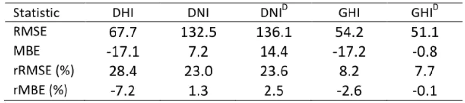
35
Table 5. Results obtained with models including the explanatory variables Day, Time, 767
Z
, T04, T05 and T09. The models are fitted and tested on the all sky conditions 768
training and testing datasets. 769
Statistic DHI DNI DNID GHI GHID
RMSE 67.7 132.5 136.1 54.2 51.1 MBE -17.1 7.2 14.4 -17.2 -0.8 rRMSE (%) 28.4 23.0 23.6 8.2 7.7 rMBE (%) -7.2 1.3 2.5 -2.6 -0.1 770 771
36 772
Fig. 1. Location of the ground measurement stations. Triangles represent stations of the
773
training dataset and circles represent stations of the testing dataset.
774 775
37 776
Fig. 2. Density scatter plots of residuals versus model fitted values for a) δ and b) log(δ).
777 778 779
38 780
Fig. 3. Density scatter plots of estimated versus ground measured irradiance and residuals
781
versus ground measured irradiance for the models fitted and tested on the all sky conditions
782
training and testing datasets.
39 784
Fig. 4. Mean ground measured DHI, DNI and GHI as function of time for the training dataset.
785
Solid lines represent cloud-free conditions and dashed lines represent cloudy conditions.
786 787 788
40 789
Fig. 5. Smooth functions of explanatory variables for the model estimating DHI fitted on the
790
all sky conditions dataset. The dotted lines represent the limits of the 5% confidence interval.
41 792
Fig. 6. Smooth functions of explanatory variables for the model estimating DNID fitted on the
793
all sky conditions dataset. The dotted lines represent the limits of the 5% confidence interval.
42 795
Fig. 7. Smooth functions of explanatory variables for the model estimating GHID fitted on the
796
all sky conditions dataset. The dotted lines represent the limits of the 5% confidence interval.
43 798
Fig. 8. Scatter plots of ground measured DHI versus explanatory variables for the all sky
799
training conditions dataset.
44 801
Fig. 9. Scatter plots of ground measured DNI versus explanatory variables for the all sky
802
conditions training dataset.