Micromechanical modeling of microtubules

(1)

HAL Id: tel-00472078

https://pastel.archives-ouvertes.fr/tel-00472078

Submitted on 9 Apr 2010

HAL is a multi-disciplinary open access archive for the deposit and dissemination of sci-entific research documents, whether they are pub-lished or not. The documents may come from teaching and research institutions in France or abroad, or from public or private research centers.

L’archive ouverte pluridisciplinaire HAL, est destinée au dépôt et à la diffusion de documents scientifiques de niveau recherche, publiés ou non, émanant des établissements d’enseignement et de recherche français ou étrangers, des laboratoires publics ou privés.

Micromechanical modeling of microtubules

Melis Arslan

To cite this version:

Melis Arslan. Micromechanical modeling of microtubules. Mechanics [physics.med-ph]. École Na-tionale Supérieure des Mines de Paris, 2010. English. �NNT : 2010ENMP1684�. �tel-00472078�

(2)

École doctorale n° 432 : Sciences des Métiers de l 'Ingénieur

présentée et soutenue publiquement par

Mélis ARSLAN

le 26 janvier 2010

MICROMECHANICAL MODELING OF MICROTUBULES

Doctorat ParisTech

T H È S E

pour obtenir le grade de docteur délivré par

l’École nationale supérieure des mines de Paris

Spécialité Mécanique

Directeurs de thèse : Mary C. Boyce, Sabine Cantournet

T

H

È

S

E

Jury

Prof. Martine Ben Amar Président

Prof. Mathias Brieu Rapporteur

Prof. Erwan Verron Rapporteur

Dr. Julie Diani Examinateur

(3)

ABSTRACT

Microtubules serve as one of the structural components of the cell and govern some of the important cellular functions such as mitosis and vesicular transport. Microtubules are comprised of tubulin subunits formed by α and β tubulin dimers arranged in a cylindrical hollow tube structure with a diameter of 20nm. They are typically comprised of 13 or 14 protofilaments arranged in spiral configurations. The longitudinal bonds between the tubulin dimers are much stiffer and stronger than the lateral bonds. This implies a highly anisotropic structure and mechanical properties of the microtubule. In this work, the aim is to define a complete set of elastic properties that capture the atomistic behaviour and track the deformation of the microtubules under different loading conditions. A seamless microtubule wall is represented as a two dimensional triangulated lattice of dimers from which a representative volume element is defined. A harmonic potential is adapted for the dimer–dimer interactions. Estimating the lattice elastic constants and following the methodology from the analysis of the mechanical behaviour of triangulated spectrin network of the red blood cell membrane (Arslan and Boyce, 2006); a general continuum level constitutive model of the mechanical behaviour of the microtubule lattice wall is developed. The model together with the experimental data given in the literature provides an insight to defining the mechanical properties required for the discrete numerical model of an entire microtubule created in finite element analysis medium. The three point bending simulations for a microtubule modeled using shell elements, give tube bending stiffness values that are in accordance with the experimental bending stiffness values and also reveal the mechanisms of local wall bending and shearing govern the deformation of short tubes transitioning to tube shearing and bending governing moderate length tubes and, finally, very long tubes displace by bending during the three point loading. These results uncover the importance of the anisotropic response of the tube in different loading conditions and also explain the length dependent bending stiffness reported in the literature. Furthermore, micrographs also show that shrinking ends of microtubules (due to microtubule instabilities) curl out. This implies the existence of prestress. A “connector model” is proposed to include the effect of the prestress and to capture the dynamic instabilities of microtubules during polymerization/depolymerization.

(4)

RESUME

Les microtubules sont des composants structuraux de cellules et gouvernent des fonctions cellulaires essentielles telles que les mitoses et le transport des vésicules. Ils sont composés de deux sous-unités non identiques (tubulines α et β), formant un dimère, et sont arrangés de sorte à former une structure tubulaire de 20nm de diamètre. Généralement, ils sont constitués de 13 ou 14 protofilaments arrangés en spirale. Les liaisons longitudinales entre dimères sont plus rigides et fortes que les liaisons latérales. Aussi, les microtubules sont des structures fortement anisotropes.

Dans ces travaux de thèse, nous avons pour but de définir l’ensemble des coefficients élastique qui permet de reproduire leur comportement atomistique ainsi que de rendre compte de leur réponse mécanique selon des chemins de chargement variés. En négligeant la discontinuité hélicoïdale souvent observée, un microtubule est représenté par une structure triangulaire de dimères à partir desquels un volume élémentaire représentatif est défini. Un potentiel harmonique est utilisé pour décrire les interactions entre dimères voisins. A partir de l’estimation des constantes élastiques et de l’utilisation de la méthode proposée par Arslan et Boyce (2006) -alors pour analyser le comportement mécanique d’un réseau triangulaire de spectrines composant les membranes des globules rouges-, un modèle continu de comportement mécanique est présenté pour reproduire le comportement des parois des microtubules. Un modèle numérique éléments finis est ensuite créé pour modéliser le comportement d'un microtubule dans sa globalité. Des éléments coques sont utilisés pour reproduire les fines parois des microtubules. Les propriétés du modèle éléments finis sont ajustées à partir des résultats du modèle présenté ainsi qu'aux données expérimentales provenant de la littérature. La rigidité de flexion calculée au cours de simulation des tests de flexion 3 points est en accord avec les valeurs de la littérature. Ces tests révèlent les mécanismes de déformation en fonction de la longueur utile du tube utilisé: Flexion et cisaillement locaux de la paroi gouvernent la déformation pour de "petits" tubes. Pour des longueurs "moyennes" le cisaillement et la flexion du tube prédominent. Enfin, dans le cas de tubes "longs", la déformation est uniquement associée aux effets de flexion. Ces résultats témoignent de l’influence de l'anisotropie du tube sur la réponse observée selon différents mode de sollicitation. Ils permettent également d’expliquer l'évolution de la rigidité de flexion avec la longueur utile du tube, comme reportée dans la littérature. Enfin, des micrographes montrent la propension des extrémités des microtubules à diverger radialement -"à boucler"-. Une telle géométrie est causée par des instabilités propres aux microtubules et implique un état précontraint. Un «modèle d'interactions» est alors proposé de manière à considérer un état précontraint et ainsi reproduire la cinétique des instabilités des microtubules au cours de la polymérisation/dépolymérisation.

(5)

LIST OF TABLES

Table 1-1 The main constituents of the cytoskeleton and their mechanical properties Table 1-2 Summary of the experimental findings on microtubule elastic properties (φint_and

ext

φ depicting the internal and external diameter of the microtubule (MT)

respectively).

Table 2-1 Spring Constants

Table 2-2 Microtubule Mechanical Properties for a unit thickness (A Lattice) Table 2-3 Microtubule Mechanical Properties for a unit thickness (B Lattice)

Table 3-1 The bending modulus and flexural rigidity values for different boundary conditions for the thin-shell discrete formulation of an individual microtubule of length 1μm for an effective modulus and thickness pair ofE₁₁* =2.4GPaand t*=1nm.

Table 3-2 The bending modulus and flexural rigidity values for different boundary conditions for the thin-shell discrete formulation of an individual microtubule of length 1μm for an effective modulus and thickness pair ofE₁₁* =2.4GPaand t*=1nm.

Table 3-3 The effective microtubule properties for different mechanical thicknesses Table 3-4 The bending modulus and flexural rigidity values obtained by Kis et al. (2002; 2003) using AFM three-point bending experiments.

Table 3-5 The bending modulus and flexural rigidity values obtained by Kis et al. (2002; 2003) compared to the simulations carried out for different microtubule thickness values. Table 3-6 The bending modulus and flexural rigidity values of Kis et al. (2002; 2003) modified by a factor of “1/2”to mimic the effect of a pure microtubule.

(8)

LIST OF FIGURES AND ILLUSTRATIONS

Figure 1-1 A schematic of cytoskeleton (Raven et al., Biology, 2004). ... 1 Figure 1-2 Micrographic comparison of the cytoskeleton network with other fibrous

materials’ networked structure ((A): Hartwig, 1992; (B)-(E): Gibson and Ashby, 1999). ... 2 Figure 1-3 Fluorescent micrographs showing actin microfilaments (left),

microtubules (center) and intermediate filaments (right) (Ingber, 1998). ... 3 Figure 1-4 Stress/strain behavior of actin, tubulin, vimentin and fibrin polymers

(Janmey et al., 1991). ... 5 Figure 1-5Fragment of a microtubule bundle from a flagellum (Lodish et al., 2007). ... 7 Figure 1-6 Microtubules doublet structure cross-section (Lodish et al., 2007). ... 8 Figure 1-7 Dimeric tubulin subunit showing α-tubulin and β-tubulin monomers and

their bound non-exchangeable GTP and exchangeable GDP nucleotides (Lodish et al., 2007). ... 9 Figure 1-8 Models of singlet (left and middle) and doublet (right) microtubules with

different surface lattices of tubulin dimers. In each microtubule, α-tubulin is shaded darkly and β-tubulin is shaded more lightly (Song and Mandelkow,

1993). ... 10 Figure 1-9 A schematic view of the geometrical configurations of the A and B lattices

(Tuszynski et al., 2005). ... 11 Figure 1-10 A lattice and B lattice configuration showing the RVE associated with it

and highlighting the helix angles (This will be further discussed in Chapter 2). ... 12 Figure 1-11 Force-extension behaviour calculated using a harmonic potential

between the dimers are represented here with springs (picture adopted from the molecular dynamics model of Deriu et al., 2007). ... 12 Figure 1-12 (A) Geometrical model of a microtubule (Portet et al., 2005), (B) In Sept

et al. (2003) studies four dimers are used to calculate the binding energies. Further details of this study will be discussed in Chapter 2. M loops are shown in the figure. ... 13 Figure 1-13 Pampaloni and Florin (2008) showed the protofilament to protofilament

interactions on a schematic figure using the information for 1TUB from PDB. ... 15 Figure 1-14 Dark-field microscopy reveals that the high rigidity of the microtubule

(9)

of microtubules. The red, horizontal line is a mean of the measurements giving a mean value of a persistence length of ~ 5.1 mm (Gittes et al., 1993). ... 19 Figure 1-16 A simple representation of optical tweezers apparatus: (A) A generic

optical tweezers diagram with only the most basic components, (B) A schematic diagram showing the force on a dielectric sphere. ... 21 Figure 1-17 (A)As a result of trapping forces up to 2.2 pN, microtubule buckling is

observed (Kurachi et al. 1995), (B) Flexural rigidity results for different

microtubule lengths. ... 22 Figure 1-18 Schematics of the two different methods of Felgner et al. (1996). ... 22 Figure 1-19(A) Microtubule lying on a substrate with a hole (Kis et al., 2002), (B)

Image of the microtubule before (a) and after (b) indentation (de Pablo et al.,

2003). ... 24 Figure 1-20 Deriu et al. (2007) calculated the interaction energies

monomer-monomer and dimer-dimer in the microtubule structure. ... 26 Figure 1-21 Chretien is one of the pioneers of the microtubule dynamics research

(figure by: Chretien et al., 1995). This electron microscope image shows the

ends of microtubules after 3 minutes of growth in a 13μM tubulin solution. ... 28 Figure 1-22 (a) At prometaphase, the nuclear envelope has broken down,

microtubules probe the cytoplasm until they contact a chromosome, (b) In early metaphase, most chromosomes have lined up in the equator, (c) In anaphase, the duplicated chromosomes have separated and are moving towards the spindle poles to form two daughter cells, (d) In telophase, the cell is dividing to become 2 daughter cells (Jordan and Wilson, 2004). Here blue dye marks the

chromosomes, green dye the kinetochores and the red dye marks the

microtubules. ... 29 Figure 1-23 Dynamic instabilities of the microtubules; schematic adapted from

(Kirschner and Mitchison, 2004). ... 30 Figure 2-1 Schematic of the model proposed by Deriu et al. (2007). The choice of the

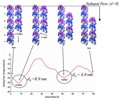
nodal points in this thesis work is the center of masses of the dimers as marked in the figure (modified from Deriu et al., 2007). ... 35 Figure 2-2 Binding free energy between two protofilaments as a function of subunit

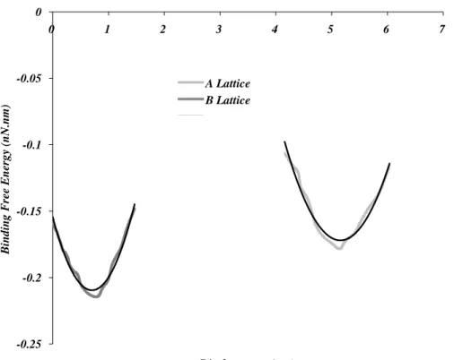
rise between adjacent dimers (modified from Sept et al., 2003). ... 36 Figure 2-3 Binding free energy for the A and B lattice structures recreated using the

(10)

depicting the subunit rise and the helix angle for the A-lattice. The RVE is shown to be a triangle. ... 39 Figure 2-5 A schematic of the B-lattice sheet model is presented here depicting the

subunit rise, helix angle and the RVE. ... 40 Figure 2-6 Here a plot of the strains are given (A) for a pure shear stress. The related

stress-shear behaviour is shown in (B) depicting the shear stiffness for the microtubule lattice. Here, K represents the shear stiffness (_s G₁₂*t*).This will be further explained in the next chapter. ... 51 Figure 2-7 A plot of the stress (T11) vs. strain (e11) is shown here depicting the

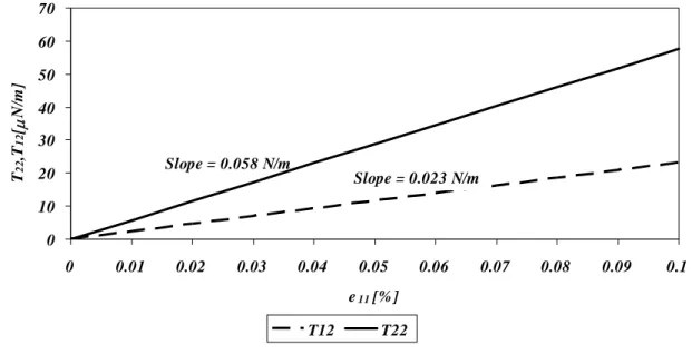
deformed and undeformed configurations of the RVE (A). The resulting lateral stress and the shear stress are also shown in (B). ... 54 Figure 2-8 A plot of the stress (T22) vs. strain (e22) is shown here depicting the

deformed and undeformed configurations of the RVE (A). The resulting

longitudinal stress and the shear stress are also shown in (B). ... 56 Figure 2-9 The area change in the RVE under uniaxial tension in the 1-direction (A)

and the resulting strains in lateral direction and the shear deformation (B) are given here. ... 59 Figure 2-10 Uniaxial Stress, T11 vs. e11 is shown in this figure. ... 60

Figure 2-11 The longitudinal stiffness in the transformed axis system for different

transformation angles. ... 62 Figure 2-12 The shear stiffness in the transformed axis system for different

transformation angles. ... 63 Figure 2-13 The tension-shear coupling components in the transformed axis system

for different transformation angles. ... 63 Figure 2-14 Schematic of different lattice structures for the microtubule lattice,

marking the seamless microtubules (modified from Mandelkow et al., 1986) (A). The B lattice structure together with the “skew angle” and the geometric

parameters are given in (B). ... 64 Figure 2-15 Uniaxial Stress, T11 vs. e11 and shear stress T12 vs. γ12 is shown here

depicting the longitudinal stiffness (K_A =E₁₁*t*) (A) and the shear stiffness

(K =_s G₁₂*t*) (B) for the seamless B lattice. ... 66

(11)

transformation angles. ... 69 Figure 2-18 The tension-shear coupling components in the transformed axis system

for different transformation angles. ... 70 Figure 3-1 Range of length scales of the simulation methods (Gates et al., 2005) ... 78 Figure 3-2 (A) The average radius of curvature is 19 nm (Muller et al., 1998), (B)

Schematic representation of the bending of a dimer (VanBuren et al., 2005), (C) Schematic representation of a dimer unit cell. ... 80 Figure 3-3 Schematics of the AFM basic modes of operation. ... 83 Figure 3-4 (A) A schematic of three-point bending by an AFM tip, (B) Microtubule

deposited on a substrate under a loading force (Kis et al., 2002). ... 83 Figure 3-5 Kis et al. experimental set up (2002). ... 84 Figure 3-6 Kis et al. (2002) experimental results:(A)Bending modulus is given in

terms as a function of the external diameter (25 nm), internal diameter (15 nm) and the suspended length, (B) Bending modulus measured for different

temperature values for a microtubule suspension length of 200 nm. ... 85 Figure 3-7 Force vs. displacement curve for the three-point bending simulation

comparing an anisotropic and an isotropic response for an effective modulus and thickness pair ofE₁₁* =2.4GPaand t*=1nm. The inset shows the deformed configuration of the microtubule. The suspension length (L) of the microtubule is 80 nm. ... 89 Figure 3-8 Contour plots showing the longitudinal stress distribution (S11) for the

three-point bending of (A)Anisotropic tube and (B) Isotropic tube with a suspension length of L = 80 nm. On the right is the top view of the experiments depicting the shear stress distribution (S12) profiles for each case. A “bottom

node” on the opposite side to the indentor contact node is depicted in the figure and is to be analyzed in this section. ... 91 Figure 3-9 Contour plots showing the shear strain distribution (LE12) for the

three-point bending of (A)Anisotropic tube and (B) Isotropic tube with a suspension length of L = 80 nm. ... 92 Figure 3-10 The plot shows the vertical displacement of the bottom node opposite to

the top surface of the tube which is in contact with the indentor for a suspension length of (A) 80 nm and (B) 200 nm. ... 94 Figure 3-11 Contour plots showing the longitudinal stress distribution (S11) for the

(12)

depicting the shear stress distribution (S12) profiles for each case. ... 95

Figure 3-12 Force vs. displacement curves for the three-point bending simulation comparing the anisotropic responses (A) and the isotropic responses (B) for an effective modulus and thickness pair ofE₁₁* =2.4GPaand t*=1nm with

suspension lengths; L= 80 and L = 200 nm. ... 96 Figure 3-13 The plot shows the vertical displacement of the bottom node opposite to

the top surface of the tube which is in contact with the indentor for an effective modulus and thickness pair ofE₁₁* =2.4GPaand t*=1nm for an isotropic and an anisotropic tube. The suspension length (L) of the microtubule is L = 500 nm

and L= 1000 nm. ... 98 Figure 3-14 Contour plots showing the longitudinal stress distribution (S11) and the

shear stress distribution (S12) for (A,E)Isotropic Tube with a suspension length

of 500 nm, (B, F) Isotropic Tube with a suspension length of 1000 nm, (C, G)Anisotropic Tube with a suspension length of 500 nm and (D, H) Anisotropic Tube with a suspension length of 1000 nm. ... 100 Figure 3-15 Force vs. displacement curves for the three-point bending simulation

comparing the anisotropic responses and the isotropic responses for an effective modulus and thickness pair ofE₁₁* =2.4GPaand t*=1nm with suspension

lengths; L = 500 nm and L= 1000 nm. ... 101 Figure 3-16 The sketch of the principal 1- and 2- direction of the microtubule and the

transferred coordinate system as shown in Chapter 2. ... 104 Figure 3-17 Force vs. displacement curve for the three-point bending results

comparing an anisotropic and an orthotropic response for a microtubule suspension length of 200nm and an effective modulus and thickness pair

ofE₁₁* =2.4GPaand t*=1nm. ... 105 Figure 3-18 Force vs. displacement curve for an effective modulus and thickness pair

ofE₁₁* =2.4GPaand t*= 1 nm, an effective modulus and thickness pair ofE₁₁* =1.2GPaand t*=2nm also an effective modulus and thickness pair ofE₁₁* =0.96GPaand t*=2.5 nm. The simulations given are for suspension

lengths of 80 nm and 200 nm. ... 107 Figure 3-19 Force vs. displacement curves for an effective modulus and thickness

pair ofE₁₁* =2.4GPaand t*= 1 nm, an effective modulus and thickness pair ofE₁₁* =1.2GPa and t*=2nm also an effective modulus and thickness pair

(13)

ofE₁₁ =0.96GPaand t=2.5 nm. The simulations given are for a suspension

length of 80 nm. ... 108 Figure 3-20 Force vs. displacement curves for the three-point simulations for an

effective modulus and thickness pair ofE₁₁* =2.4GPaand t*= 1 nm, an effective modulus and thickness pair ofE₁₁* =1.2GPa and t*=2nm also an effective modulus and thickness pair ofE₁₁* =0.96GPaand t*=2.5 nm. The simulations given are for a suspension length of 200 nm. ... 108 Figure 3-21 Force vs. displacement curve for the three point simulations for an

effective modulus and thickness pair of and t*= 1 nm, an effective modulus and thickness pair of and t*=2nm also an effective modulus and thickness pair of

and t*=2.5 nm. The simulations given are for a suspension length of 80 nm. ... 112 Figure 3-22 Force vs. displacement curve for the three point simulations for an

effective modulus and thickness pair ofE₁₁* =2.4GPaand t*= 1 nm, an effective modulus and thickness pair ofE₁₁* =1.2GPaand t*=2nm also an effective modulus and thickness pair ofE₁₁* =0.96GPaand t*=2.5 nm. The simulations given are for a suspension length of 200 nm. ... 113 Figure 3-23 Force vs. displacement curves reduced from the results of the three-point

bending experiments of Kis et al. (2002; 2003) for suspension lengths of 83 nm and 200 nm including the results modified by a factor of “1/2”. ... 115 Figure 3-24 (A)Side view of a dimer and a (B) top view of a 13 protofilament created

using cryo electron microscope images (courtesy of Dr. Denis Chretien)showing the thickness and the external diameter of the microtubule... 116 Figure 3-25 Experimental force versus vertical displacement (indentation depth)

curves obtained by Vinckier et al. (1996), nonlinear curves depicting Hertz

approximations. ... 117 Figure 3-26 (A) de Pablo et al. (2003) experiments show that microtubule indentation

is linear and reversible for forces up to 300 pN. (B) Schaap et al. (2006) show that for 2 different types of cantilever stiffnesses the microtubule stiffness

averages to give a mean of 0.074 N/m. ... 119 Figure 3-27 The indentation experiment is simulated in the finite element medium.

The example shown is the indentation of a 11.14 nm radius tube with anisotropic properties and for effective modulus and thickness pair ofE₁₁* =2.4GPaand

t*=1.0 nm. ... 121

Figure 3-28 Force versus displacement for the radial indentation for an isotropic and an anisotropic tube for two different effective pairs: for an effective modulus and

(14)

thickness pair ofE₁₁ =2.4GPaand t=1.0 nm, also an effective modulus and

thickness pair ofE₁₁* =1.6GPaand t*=1.5 nm. ... 122 Figure 3-29 Force versus displacement plots for the radial indentation of anisotropic

tubes with different set of effective properties. Here E* is the effective

longitudinal modulus and t* is the effective mechanical thickness. ... 124 Figure 3-30 The stress contours indicating the longitudinal stress (S11)

distribution[A-D] and the shear stress (S12) distribution [E-F] at the indentor contact area for different E*, t* pairs and comparing isotropic and anisotropic tubes. ... 127 Figure 3-31 Force versus displacement for the radial indentation simulation giving a

comparison with the experimental results. ... 128 Figure 3-32 The relative contributions of the tube bending deformation on the total

displacement of the indentor in three-point bending for an isotropic and

anisotropic tube. ... 133 Figure 3-33 The relative contributions of the shearing deformation on the total

displacement of the indentor in three-point bending for an isotropic and

anisotropic tube. ... 134 Figure 3-34 The relative contributions of tube wall bending/ ovalization deformation

on the total displacement of the indentor in three-point bending for an isotropic and anisotropic tube for different E*, t* pairs. ... 135 Figure 4-1 Ribbon diagram of the tubulin dimer showing α−tubulin with bound GTP

(top), and β-tubulin containing GDP (bottom). The arrow indicates the direction of the protofilament and microtubule axis(Nogales, 1998). ... 143 Figure 4-2 Structural model showing the microtubule instability. (a) Microtubules

grow as 2D-sheets, (b)GTP hydrolyzed resulting in “blunt-ended” microtubules, (c)Microtubules lateral bonds are in a strained state about to break, (d) The unstable blunt-ended microtubule results in the loss of the GTP region (Arnal et al., 2000). During assembly, microtubules are observed to have “blunt ends”, while during disassembly they are observed to have “tapered” or “coiled” ends. 144 Figure 4-3 The micrographs show that growing ends of microtubules often taper to

long, narrow ... 145 Figure 4-4 (A) A fit of the derived r( z)is shown here. (B) Energy is in the units of

2

o o z

ac

(a is a material parameter) on the left axis and k_Bθon the right axis. The end deflection is in the units of r in the bottom axis and nanometers in the

(15)

article. ... 147 Figure 4-5 Estimation of ΔG_longitudin_alversus ΔG_lateralis shown. The researchers

(VanBuren et al., 2002) predicted the energy of “curling out” as 2.5k_Bθ from the lateral energy change for a disassembly of -30μm/min. ... 148 Figure 4-6 (A) Initial microtubule configuration, (B) Side view of the protofilaments

in the initial state, (C)The equilibrium configuration of the microtubule forming “ram’s horns” (Molodtsov et al., 2005). ... 150 Figure 4-7 The plot shows the relief of the prestress at the tip of the tube, two

different shell elements are marked (2701 and 2703) for future reference. ... 153 Figure 4-8 (A) The tensile stress relief in the 1-direction (tube axis direction, S11) is

shown (B) which results in the accumulation of lateral tensile stress (S22) and

shear stress (S12). ... 155

Figure 4-9 The plot shows the built-up of the lateral stress at the tip of the tube, two different shell elements are marked (2701 and 2703) for reference. ... 156 Figure 4-10 The plots shows the strain energy relief of the whole tube shell model;

θ is chosen as 280 K... 156 Figure 4-11 (A) Depolymerization at the tip of the microtubules in the presence of

calcium Muller-Reichert et al. (1998), (B)The single strand finite element analysis showing the strain energy release from a single strand with the inset depicting the evolution of the conformation change in the strand with the stress release. ... 158 Figure 4-12 The potential function used for the lateral connectors depicting the

corresponding force versus extension (dimer separation) and the related stiffness in the inset are created using equation (72) and taking the necessary

derivatives with respect to the dimer separation. ... 160 Figure 4-13 The undeformed configuration of the cylindrical tube with an axial

prestress of 0.06 GPa at the most outer radial position. ... 162 Figure 4-14 The energy of one of the tip connectors is monitored during the finite

element analysis with respect to the tip radius change of the tube giving a profile showing the energy profile suggested by equation (72). The inset shows the tip of the tube with the related connector element. ... 162 Figure 4-15 (A) The pictures shows the deformed contours of the cylindrical tube

after the prestress is allowed to release, the tip elements are stress-free, (B) Similar conformations have been observed in the literature by researchers

(16)

release for the model. A comparison of the contour plot and cryo-electron

microscope images (Mandelkow et al., 1991) are shown. ... 165 Figure 4-17 (A) The contours for the cylindrical tube showing the accumulated

lateral stress and the shear stress causing an unfavourable condition for the tube, (B) This unfavourable condition was discussed earlier with this sketch by Hunyadi et al. (2005). ... 165 Figure 4-18 (A) The simulation result having changed the connector stiffness down to

about 0.001 N/m resulting in breaking of them under the induced prestress showing the “catastrophe” form. (B) The cryo-electron microscopic image shows the depolymerization and “coiling out” of microtubules in the presence of calcium (Muller-Reichert et al., 1998)... 166 Figure 4-19 A few molecules of Vinblastine bound to the microtubule end to suppress

(17)

1. CHAPTER 1: INTRODUCTION

1.1. Cytoskeleton

The cytoskeleton (Figure 1-1), the system of protein filaments that permeate the cytoplasmic space of all eukaryotic cells, is primarily responsible for the structural integrity exhibited by a cell and governs its deformation in response to a given stress.

Figure 1-1 A schematic of cytoskeleton (Raven et al., Biology, 2004).

1.1.1. Cytoskeletal Filaments

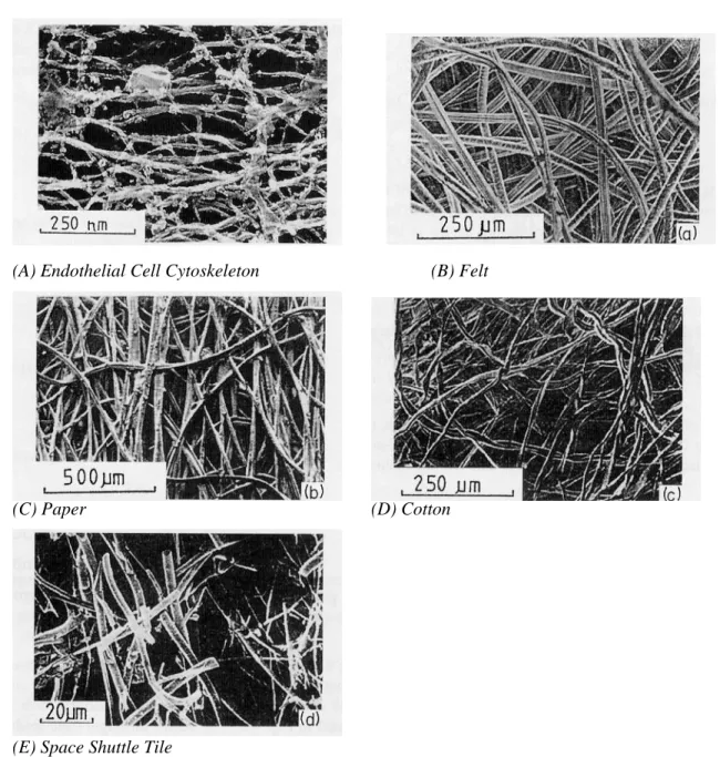
The protein network of the cytoskeleton is comprised of several types of intertwined filaments with a variety of interconnections (Figure 1-2, A). The stiffness of the network depends upon the elastic properties of the constituent fibres and their geometric assembly. This chapter will examine the biological composition and the properties of the primary biopolymers that constitute the cytoskeletal network.

(18)

The cytoskeletal matrix is primarily composed of three constituents, actin microfilaments, microtubules, and intermediate filaments (Figure 1-3). These members form a complex interconnected network with varying degrees of interconnection existing in a state of dynamic equilibrium.

(A) Endothelial Cell Cytoskeleton (B) Felt

(C) Paper (D) Cotton

(E) Space Shuttle Tile

Figure 1-2 Micrographic comparison of the cytoskeleton network with other fibrous materials’ networked structure ((A): Hartwig, 1992; (B)-(E): Gibson and Ashby, 1999).

(19)

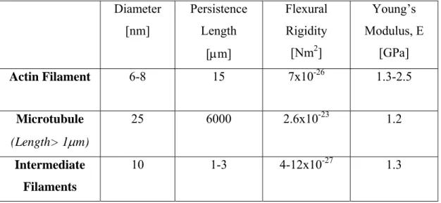
Table 1-1 gives a summary of the basic characteristics of the constituents of the cytoskeleton.

Table 1-1 The main constituents of the cytoskeleton and their mechanical properties

Diameter [nm] Persistence Length [μm] Flexural Rigidity [Nm2] Young’s Modulus, E [GPa] Actin Filament 6-8 15 7x10-26 1.3-2.5 Microtubule (Length> 1μm) 25 6000 2.6x10-23 1.2 Intermediate Filaments 10 1-3 4-12x10-27 1.3

1.1.2. Basic Characteristics of the Constituents of the Cytoskeleton

Figure 1-3 Fluorescent micrographs showing actin microfilaments (left), microtubules (center) and intermediate filaments (right) (Ingber, 1998).

(20)

1.1.2.1. Actin Filaments

Actin constitutes a main part of proteins in the cell, about 1-10 wt. % of total cell proteins in non-muscle cells and up to 20% in muscle cells. Molecular actin is comprised of 375 residues (molecular weight 43 kDa). Actin exists either in globular form (G-actin monomers) or filamentous form (F-actin polymer).

Actin filaments participate in many important cellular functions, including muscle contraction, cell motility, cell division and cytokinesis, vesicle and organelle movement, cell signalling, and the establishment and maintenance of cell junctions and cell shape. They play an essential role in all types of motility. In muscle cells, actin filaments are the scaffold on which myosin proteins generate force to support muscle contraction. In non-muscle cells, they serve as a track for cargo transport myosin.

F-actin filaments can further organize into tertiary structures such as bundles or a lattice network with the help of actin binding proteins.

1.1.2.2. Intermediate Filaments

The intermediate filaments appear to play a primary structural role in the cytoskeleton. They constitute roughly 1% of total protein in most cells, but can count for up to 85 % in cells such as epidermal keratinocytes and neurons (Fuchs and Cleveland, 1998).

The intermediate filaments are a family of related proteins that share common structural and sequence features. Intermediate filaments have an average diameter of 10 nanometers, which is between that of actin filaments and microtubules.

Although intermediate filaments are more stable than microfilaments, they can be modified by phosphorylation. This occurs on a time scale typically longer than for changes in the F-actin structures, however.

(21)

1.1.2.3. Microtubules

A microtubule, found in almost every living system, is a polymer of tubulin protein subunits, which are arranged in a cylindrical tube structure with an outside diameter of about 25nm and an inside diameter of about 15nm.

Varying in length from a fraction of a micrometer to hundreds of micrometers, microtubules are much stiffer than either actin filaments or intermediate filaments.

The constitutive behaviour of the cytoskeletal filaments can be integrated into structure-based micromechanical models of the entire cell to predict the mechanical response of the combined network in the cytosplasm.

Actin filaments, intermediate filaments and microtubules each have their specific physical properties and structure suitable for their specific role in the cytoskeleton. For example, the two dimensional arrangement of actin filaments in stress fibres, appears to form cable-like structures involved in the maintenance of the cell shape and the transduction pathways. F-actin filaments can support large stresses without high deformation and it ruptures at approximately 3.5 N/m2_{(Janmey et al., 1991). It provides} the highest resistance to deformation until a certain critical value of local strain. Actin networks are believed to “fluidize” under high stresses to facilitate cell locomotion (Janmey et al., 1991).

Figure 1-4 Stress/strain behavior of actin, tubulin, vimentin and fibrin polymers (Janmey et al., 1991).

(22)

Intermediate filaments are mainly involved in the maintenance of the cell shape and integrity. It is shown that (Ma et al., 1999) the intermediate filaments resist high applied pressures by increasing their stiffness. These filaments can stand higher stresses than the other two components without damage (Figure 1-5).

Microtubules undergo relatively larger strains (~60%, see: Figure 1-5) when compared to the other filaments. The rupture stress is about 0.4 – 0.5 N/m2 (Janmey et al., 1991). Long microtubules (Length > 1μm) have the highest flexural rigidity when compared to the

other filaments. They also resist high compression with the support from the microtubule associated proteins (Brangwynne et al., 2006). Because they are the most rigid elements of the cytoskeleton, they are largely responsible for the shape and mechanical rigidity of cells. They are also the thickest filaments in the cytoskeleton.

Microtubules have been a topic of interest for numerous experimental and theoretical researches, including those on elastic buckling (Kurachi et al., 1995; Brangwynne et al., 2006), force-related dynamic instability analysis (Molodtsov et al., 2005; Liedewij et al., 2008; Grishchuk et al., 2005), and bending experiments (Kis et al., 2002 and Pampaloni et al, 2008)

1.2. Microtubules Inside the Cell

1.2.1. Microtubule Functions

Microtubules in eukaryotic cells can be classified into two general groups; axonemal groups and cytoplasmic microtubules. The first group, axonemal microtubules, includes the highly organized, stable microtubules found in specific structures associated with cell movement; cilia, flagella (Figure 1-5) and the basal bodies to which these appendages are attached. The central shaft or axoneme of a cilium or flagellum consists of a highly ordered bundle of axonemal microtubules. The second group is the more loosely

(23)

organized, dynamic network of cytoplasmic microtubules. The second group of microtubules has not been recognized until the early 1960s.

Cytoplasmic microtubules are responsible for a variety of functions. They maintain the axons, nerve cell extensions in mammalian cells. Some migrating mammalian cells require cytoplasmic microtubules to maintain their polarized shape. Cytoplasmic microtubules form the mitotic and meiotic spindles that are essential for the movement of chromosomes during mitosis and meiosis. Cytoplasmic microtubules also contribute to the spatial disposition and directional movement of vesicles and other organelles by providing an organized system of fibres to guide the movement.

1.2.2. Microtubule Structure

The basic subunit of a microtubule protofilament is a heterodimer of the protein tubulin. The heterodimers are composed of one molecule of α-tubulin and one molecule of β -tubulin, each with a molecular mass of about 50 000 Da. Pairs of α-tubulin and β-tubulin

form a unit 8 nm length (Figure 1-7). As soon as individual α- andβ-tubulin molecules

are synthesized, they bind tightly to each other to produce an αβ-heterodimer that does

not dissociate under normal conditions.

(24)

Individual α- and β-tubulin molecules have diameters of about 4-5 nm. α- and β-tubulin molecules have nearly identical three-dimensional structures (Nogales et al., 1998). Each tubulin subunit binds two molecules of GTP (Guanosine-5'-triphosphate). One GTP-binding site, located in α-tubulin, binds GTP irreversibly and does not hydrolyze it, whereas on the second site, located on β-tubulin, binds GTP reversibly and hydrolyzes it to GDP (Guanosine-5'-diphosphate).

Figure 1-6 Microtubules doublet structure cross-section (Lodish et al., 2007).

The microtubule wall consists of longitudinal arrays of linear polymers called

protofilaments. There are usually 13 protofilaments arranged side by side around the

hollow center, lumen. In a microtubule, lateral and longitudinal interactions between tubulin subunits are responsible for maintaining the tubular shape. In rare cases, singlet microtubules contain more or fewer number of protofilaments (e.g. 11, 15). In addition to the simple singlet structure, doublet (in cilia and flagella) or triplet microtubules exist (centrioles, basal bodies), (Figure 1-6).

(25)

Figure 1-7 Dimeric tubulin subunit showing α-tubulin and β-tubulin monomers and their bound non-exchangeable GTP and exchangeable GDP nucleotides (Lodish et al., 2007).

A microtubule is a polar structure, its polarity arising from the head-to-tail arrangement of the exposed α- and β-tubulin dimers in a protofilament. Microtubules have a (+) and a (-) end (Lodish et al., 2007).

Because microtubules assemble from microtubule organizing centers (MTOC), microtubule polarity becomes fixed in a characteristic orientation. In most mammalian cells, the (-) ends of microtubules are closest to the MTOC.

The (+) end is the fast growing end and the (-) end is the slow growing end. This information is important in determining the direction of motion of the microtubules. Microtubules assemble by polymerization of α- and β-tubulin dimers. Once they are assembled, their stability is temperature dependent.

1.2.2.1. Lattice Structure

Ledbetter and Porter (1963) were the first to describe the tubules found in the cytoplasm. The experimental data in the literature covers microtubules of protofilament number ranging from 12 to 17. Chretien et al. (1992) showed that in vitro assembled microtubules mostly have 14 protofilaments whereas the cell extracts contain 13 protofilament microtubules. The predominant 13 protofilament structure in vivo has a helical pitch of 3 monomers per turn of the helix (Mandelkow et al., 1986). These microtubules are usually

(26)

referred to as “13_3 microtubules”; where 13 denoted the number of protofilaments and 3 denotes the helical pitch.

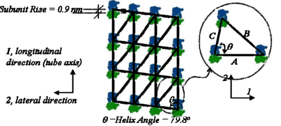
The small difference between the α− and β-monomers allows the existence of different lattice structures; A and B lattices (Figure 1-8). For the commonly accepted 13_3 model, moving around the microtubule, in a left-handed sense, protofilaments of the A lattice have a vertical shift of 4.9 nm upwards relative to their neighbours (Song and Mandelkow, 1993). In the B lattice, this offset is only 0.9 nm. This change results in a “seam” a structural discontinuity in the B lattice. The seam implies a neighbouring interaction (α−β) that differs from the majority of the lateral interactions (α−α and β−β) (Figure 1-9).

Figure 1-8 Models of singlet (left and middle) and doublet (right) microtubules with different surface lattices of tubulin dimers. In each microtubule, α-tubulin is shaded darkly and β-tubulin is shaded more lightly (Song and Mandelkow, 1993).

These two models have initially been proposed by Amos and Klug (1974). The researchers noted that A and B “sub-fibres” have the same lattice structure; however, B lattice structure shows an oblique line up of the dimers whereas in the A lattice structure, the dimers are in a staggered arrangement.

A careful look at the Figure 1-8 and the Figure 1-9, it is observed that the A lattice has a “checkered” appearance, while the B lattice gives a rather “banded” appearance. However the 8 nm dimer to dimer length is observed to be the same in both configurations.

(27)

Figure 1-9 A schematic view of the geometrical configurations of the A and B lattices (Tuszynski et al., 2005).

Because of the existence of the “seam” the discontinuity in the B lattice, A lattice stacking is usually the favoured lattice for modeling. In an A lattice, the α and β subunits alternate along the helix, while in a B lattice the subunits are the same along the helix (Figure 1-9).

1.2.2.2. Tubulin-Tubulin Interactions

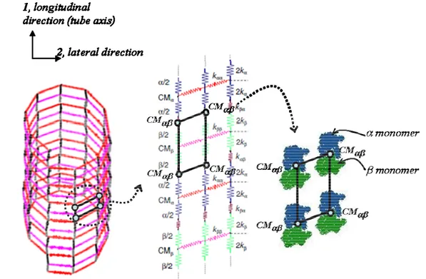
Once the individual monomers are synthesized, they bind tightly to each other and do not separate; a dimer could be graphically represented by a node that lies at the center of mass of the α and β monomers (Figure 1-10).

Note that in this work, it will be assumed that the monomer to monomer bonds are inextensible and that they do not break during disassembly of microtubules. Therefore the dimer can be taken as a rigid unit.

(28)

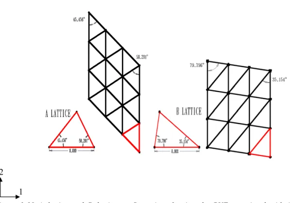
Figure 1-10 A lattice and B lattice configuration showing the RVE associated with it and highlighting the helix angles (This will be further discussed in Chapter 2).

Figure 1-10 shows that the helical angle of 45.6o corresponds to the A lattice and 79.8o corresponds to the B lattice. Further details of the lattice structure will be discussed in Chapter 2.

Figure 1-11 Force-extension behaviour calculated using a harmonic potential between the dimers are represented here with springs (picture adopted from the molecular dynamics model of Deriu et al., 2007).

1 2

(29)

Figure 1-12 (A) Geometrical model of a microtubule (Portet et al., 2005), (B) In Sept et al. (2003) studies four dimers are used to calculate the binding energies. Further details of this study will be discussed in Chapter 2. M loops are shown in the figure.

Metoz and Wade (1997) noted that a seamless microtubule can be modeled as a three dimensional helical lattice of dimers (Figure 1-12, A). The microtubule lattice is demonstrated with a two-dimensional sheet where the small bond stretches are approximated by a harmonic energy potential (Figure 1-11) and is represented as the parabolic equation given as:

2 0 2 1 | ) ( ) ( | _i _i i r t r k − = ) r Uharmonic( i (1)

The exact potential functions for the intra- and inter-protofilament bonds are unknown. In the literature, different researchers (Molodtsov et al., 2005 and Deriu et al., 2007) considered different interaction potentials for the longitudinal and lateral bonds. For the former, within the protofilament, the interaction force is chosen such that it either brings

(A) (B)

(30)

the dimers closer or separates them apart without rupture of the bonds (except from the extreme cases), but for the latter, the dimer pair tends to be in attraction until a disturbance is applied which results in separation of the pair and even breakage of the bond. This lateral interaction is captured by:

) / exp( r_o Aξ −ξ = 2 * U (2)

Here, ro is the distance in which the bond exerts the maximum attractive force,

ξ

characterizes the dimers’ deviation from the equilibrium configuration and A is the stiffness parameter. This kind of an energy potential captures the bending and breaking of the protofilaments during disassembly of a microtubule. This will later be discussed in Chapter 4.

1.2.3. Microtubule Mechanics

Structural investigations (Nogales et al., 1998 and Li et al., 2002) and theoretical calculations (Sept et al., 2003; VanBuren et al., 2002; Molodtsov et al., 2005 and Deriu et al., 2007) show that lateral and longitudinal tubulin interactions have different properties. While the lateral inter-protofilament contacts (α−α, β−β) are mostly electrostatic, the longitudinal intra-protofilament contacts (α−β, β−α) are hydrophobic, Van der Waals (Nogales et al., 1998). The different strengths of the inter- and intra-protofilaments bonds suggest that the longitudinal and lateral moduli are different for a microtubule, i.e. the existence of anisotropy in the microtubule structure. It’s shown by Sept et al. (2003) using five dimers and an electrostatic calculations package (Baker et al., 2001) that the longitudinal bonds along the protofilaments are found to be ~ 7 kcal/mol stronger than the lateral bonds (Figure 1-12, B). The findings of Sept et al. (2003) have enlightened the study presented in this thesis work and the details of it will be discussed in Chapter 2. Thus, the longitudinal and lateral interactions should be treated differently in modeling.

(31)

structural motif involved in inter-protofilament interactions is the ‘M-loop’ (Figure 1-12,

B and Figure 1-13). The terminal parts of the M-loops are considerably flexible and

appear to work like a hinge, allowing relative motion between the protofilaments such as shearing. They provide resilience to the microtubules to allow shear deformation in loading conditions such as bending.

Despite the various attempts in the literature to determine the lateral bonding strengths of the protofilaments (Sept et al., 2003; VanBuren et al., 2002; Molodtsov et al., 2005 and Deriu et al., 2007), there hasn’t been a mathematical method found to determine the bonding coefficients. To be able to make that possible, various approaches will be compared in this section.

A stochastic model of microtubule assembly dynamics that estimates the tubulin-tubulin bond energies and mechanical energy stored in the lattice dimers has been developed by VanBuren et al. in 2002. From Monte Carlo simulations the researchers determined the lateral bonding energy which they found to be between 3.2kBθ < ΔGlat < 5.7 kBθ where

kB is the Boltzmann’s constant (1.38 x 10-23 N.m/K) and θ is the absolute temperature.

The longitudinal bonding energy is found to be 6.8kBθ < ΔGlong < 9.4 kBθ. From here one

can estimate that the longitudinal bonds are around 2-3 times stronger than the lateral bonds. This is also agreed up on in the research of Molodtsov (2005).

Figure 1-13 Pampaloni and Florin (2008) showed the protofilament to protofilament interactions on a schematic figure using the information for 1TUB from PDB.

(32)

If one observes the indentation experiments carried out by de Pablo et al. (2003), which will be investigated in Chapter 3, it’s seen that force versus AFM tip displacement has been found to be k ~ 0.1 N/m. Portet et al. (2005) have taken this to be the lateral stiffness coefficient. However it’s important here to note that the indentation response is a combination of the shear stiffness and lateral stiffness; so the assumption of this last reference requires further study.

There is no direct technique to measure the elastic properties of microtubules and as a result, most experimentalists estimate the effective elastic properties of the microtubules by comparing the experimental data with static solid beam models. Theorists estimate the microtubule properties by applying atomistic dynamic models. However, in the literature we cannot find a complete description of the mechanical behaviour of the microtubules that capture the atomistic behaviour and tracking the deformation under different loading conditions and giving a complete set of mechanical properties.

Measurement results related to the mechanical properties of microtubules differ greatly. The largest discrepancies concern estimations of Young's modulus. Depending on the authors, reported values range between 1 MPa (Vinckier et al., 1996) and 7 GPa (Kurachi et al., 1995).

1.2.3.1. Review of Experimental Techniques

Experimental attempts for determining the elastic properties of microtubules date back to 1980s. In spite of the increasing level of sophistication in the analyses, there still is some conflict in the results.

We will briefly review the latest experimental techniques and the latest results from the literature. The experimental methods reviewed will include thermal fluctuation and hydrodynamic flow measurements (Gittes et al., 1993; Venier et al., 1994; Mickey and

(33)

Howard, 1995), optical tweezers (Felgner et al., 1996 and Kurachi et al, 1995) and atomic force microscopy (Kis et al., 2002; de Pablo et al., 2003 and Schaap et al. 2006).

The application of Hooke's Law to various mechanical tests of micro- and nano-scale objects enables approximation of the elastic properties. Recent advances in microscale experiments provide techniques that permit the application of forces in the pico- to micro-Newton (pN-μN) range. Since deformations of biomacromolecules lie within this range, they can be tested using available instruments. In principle, one could directly measure the flexural rigidity of the microtubules by directly applying a known axial force at the free end and measuring its deflection. However, due to the small size and the high stiffness of the microtubules, such a measurement has not been possible. Instead, the researchers chose to apply thermal forces to the microtubule and measure the bending of constrained microtubules. Such measurements have been carried out earlier for actin filaments but it has been more challenging for microtubules because of the higher rigidity resulting in small deflections. The next section discusses thermal fluctuation measurement methods.

Analysis of Fluctuations

Gittes et al. (1993) reported the first accurate measurements of the flexural rigidity of the microtubules. By analyzing the thermally driven fluctuations in their shape, the flexural rigidity of 25-26 μm long microtubules was reported.

Microtubules vibrate when subjected to thermal excitation. The frequencies of the natural vibrations and the shape changes are referred to as modes. Modes depend on the material mass, stiffness and damping properties of the material, as well as on the boundary conditions. As the filament shape fluctuates over time due to thermal motions, the amplitude of each mode fluctuates and this provides an estimate for the flexural rigidity of the filament. By analyzing the fluctuations associated with shape changes in the microtubules recording using dark-field and video-enhanced microscopy, the flexural rigidity of the microtubule can be estimated using the mean square vibration amplitude.

(34)

In thermal fluctuation analyses, the shape of the filament (in terms of the local tangential angle,θ( s)) is represented as a sum of cosine modes (Landau and Lifshitz, 1980):

⎟ ⎠ ⎞ ⎜ ⎝ ⎛ = =

∑

∞ = ∞ = L s n a L s s n n n n π θ θ( ) ( ) cos 0 0 2 , (3)

where L is the length of the microtubule and an is the amplitude of the nth mode. The

related bending energy is the sum of these coefficients:

(

)

∑

∞ = − ⎟ ⎠ ⎞ ⎜ ⎝ ⎛ = 1 2 0 2 2 1 n n n a a L n EI U π . (4)

Here a_n0denotes the amplitude in the absence of thermal forces and EI is the flexural

rigidity.

The equipartition theorem (Reif, 1965) states that each harmonic mode has a mean energy of:

θ

B

k

1

. This implies that the mean square amplitude of the nth

node will be:

(

)

2 2 0 ⎟ ⎠ ⎞ ⎜ ⎝ ⎛ = − = π θ n L EI k a a a_n) _n _n B var( . (5)

Here kB is the Boltzmann's constant, θ is the temperature. From here, the persistence

length, l , is derived as: _p

(

₀

)

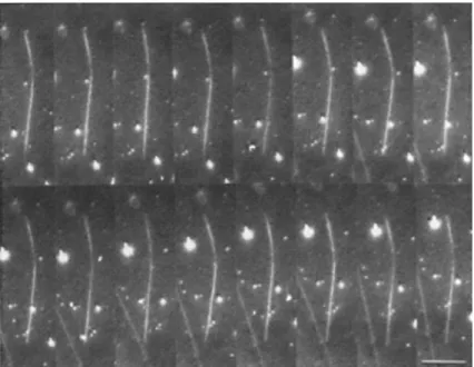
2 2 2 2 n n B p a a n L k EI l − = = π θ . (6)

(35)

Figure 1-14 Dark-field microscopy reveals that the high rigidity of the microtubule leads to very small fluctuations in curvature (Gittes et al., 1993).

Figure 1-14 shows that the high rigidity of the microtubule leads to very small fluctuations in curvature.

Figure 1-15 Microtubule thermal fluctuation data points include the first three modes of microtubules. The red, horizontal line is a mean of the measurements giving a mean value of a persistence length of ~ 5.1 mm (Gittes et al., 1993).

(36)

The flexural rigidity of taxol stabilized microtubules were calculated to be 2.15x10-23

Nm2. The persistence length was then derived to be ~5.1 mm (Figure 1-15).

The researchers (Gittes et al., 1993), using the experimental result of flexural rigidity, calculated the Young’s modulus (isotropic) of the microtubules to be E ~ 1.2 GPa assuming microtubules to be hollow cylinders with an external diameter of 28 nm and an internal diameter of 23 nm. This modulus is similar to rigid plastics such as Plexiglas or polypropylene.

However, it’s important to discuss a bending modulus which is different than the longitudinal modulus when shear effects are considered. Shear effects decrease the resistance to bending in a manner which depends on how bending is applied, thus the bending modulus can be much lower than the longitudinal modulus as will be shown later in this Chapter 3.

Venier et al. (1994) used a similar method to measure microtubule stiffness. They estimated flexural rigidity of 5-7 μm long microtubules by analyzing the thermal

fluctuations of axoneme- bound microtubules whose axonemal end was fixed to a glass cover-slip. The principle is based on the fact that when microtubules are attached at one end and subjected to thermal forces in solution, the free end undergoes fluctuations around an average position. The researchers used two different methods: dynamic and

static. In the first method, a hydrodynamic flow was applied to microtubules and the

flexural rigidity was derived from the analysis of the bending shape of the microtubules (dynamic method). In the second method, the flexural rigidity was derived from thermal fluctuation of the free end of axoneme-bound microtubules (static method). As a result, a good agreement between the values of flexural rigidity of microtubules derived from the dynamic and the static methods (0.85 x10-23_Nm2_{and 0.92x10}-23_Nm2_{, respectively).}

The effect of the stabilizing agents on the microtubule rigidity has been studied by Mickey and Howard (1995) using the same techniques as Gittes et al. (1993). The researchers measured the flexural rigidity of pure microtubules to be ~2.60x10-23_Nm2

(37)

The flexural rigidity of taxol stabilized microtubules was measured to be ~3.20x10-23

Nm2.

Optical Tweezers Technique

(A) (B)

Figure 1-16 A simple representation of optical tweezers apparatus: (A) A generic optical tweezers diagram with only the most basic components, (B) A schematic diagram showing the force on a dielectric sphere.

An optical tweezer (Figure 1-16) is a scientific instrument that uses a focused laser beam to provide an attractive or repulsive force (typically on the order of picoNewtons, pN), depending on the refractive index mismatch to physically hold and move microscopic dielectric objects.

Optical tweezers offer a further option for measuring the mechanical properties of cytoskeletal proteins. This technique was first used to measure the stiffness of microtubules by Kurachi et al. (1995). Buckling of microtubules was induced by the attachment of polystyrene microspheres (Figure 1-17). The stiffness of these structures was then deduced by estimating the critical buckling load (using Euler buckling theory and assuming an effective EI), as well as from the analysis of the deflected lengths and the bending angles. The measurements were made on taxol-stabilized and MAP-decorated microtubules. The persistence lengths, which were dependent on the deflected lengths, varied between 8 mm and 47 mm.

(38)

(A) (B)

Figure 1-17 (A)As a result of trapping forces up to 2.2 pN, microtubule buckling is observed (Kurachi et al. 1995), (B) Flexural rigidity results for different microtubule lengths.

Felgner et al. (1996) used optical tweezers in the absence of the polystyrene microspheres. They used two different methods (Figure 1-18). The microtubules were attached at one end to axonemes glued to the cover-slip. In the first method (RELAX), the microtubule is bent perpendicularly to its long axis with the optical tweezers only once. After switching off the laser power, the microtubule relaxes and quantitative analysis of the relaxation movement yields its flexibility. In the second method (WIGGLE), the optical tweezers are used to move the microtubule back and forth against the surrounding buffer. The flexural rigidity is calculated from the bending shape of the microtubule at the moment of maximum deflection.

(39)

The two methods yielded consistent measurements of flexural rigidity: 4.5x10-24

Nm2 for

pure microtubules, about 2x10-24

Nm2 for taxol treated microtubules.

Atomic Force Microscopy (AFM)

AFM relies on probing the interaction between a sharp tip located at the end of a cantilever and the sample. The first measurements of microtubule stiffness using atomic force microscopy were made by Vinckier et al. (1996). These involved radial indentation of the microtubules and recording force versus vertical tip displacement curves in the presence of different concentrations of glutaraldehyde. The measurements revealed Young’s moduli to range from 1 MPa to 12 MPa using a Hertz approximation (Sneddon, 1965).

In Kis et al. (2002) work, the microtubules were deposited on APTES-functionalized alumina membranes containing holes (Figure 1-19, A) and were subjected to three point bending using AFM. The maximum deflection of the suspended part of the microtubule was measure. The analysis considered this deflection to be the sum of the deflection due to bending and that due to shearing. The researchers derived the shear modulus to be 2 orders of magnitude lower than the Young’s modulus using Timoshenko beam bending

theory (Timoshenko, 1970).

De Pablo et al. (2003) have also used atomic force microscopy to measure the deformation of microtubules (Figure 1-19, B) The researchers applied radial indentation to microtubules. However, unlike Vinckier et al. (1996), they used taxol instead of glutaraldehyde to stabilize the microtubules. The microtubules were deposited on a glass surface that was coated with aminopropyltriethoxysilane to promote their adhesion. The force versus tip distance curves data were recorded in the linear or elastic mode. In the elastic regime, the microtubule behaved like a spring, with a spring constant of about 0.1

N/m. The authors reported the microtubules to behave linearly up to an indentation of 4 nm.

(40)

In Chapter 3, AFM methods and the findings of Kis et al. (2002) and de Pablo et al. (2003) will be discussed in more detail and will be compared with the finite element simulations based on the proposed discrete model.

(A) (B)

Figure 1-19(A) Microtubule lying on a substrate with a hole (Kis et al., 2002), (B) Image of the microtubule before (a) and after (b) indentation (de Pablo et al., 2003).

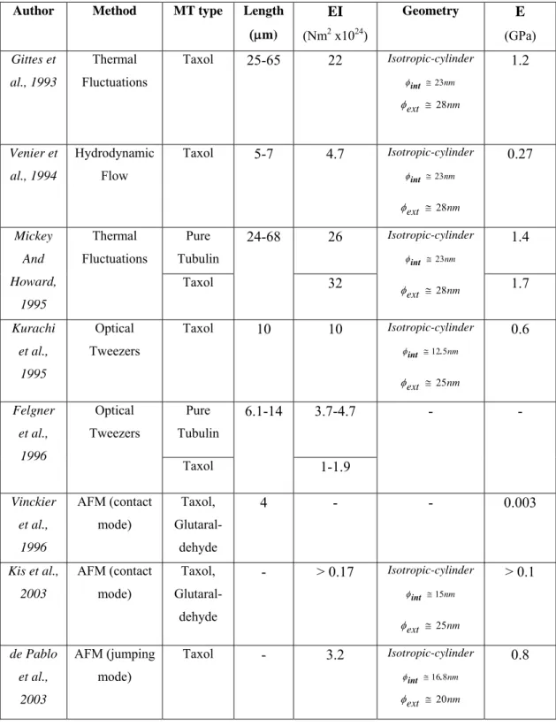
Table 1-2 gives a summary of the experimental method findings. Note that some of the values are missing due to the fact that they were not specified in the publication.

(41)

Table 1-2 Summary of the experimental findings on microtubule elastic properties (φ_intand φ_ext depicting the internal and external diameter of the microtubule (MT) respectively).

Author Method MT type Length

(μm) EI (Nm2_x1024₎ Geometry E (GPa) Gittes et al., 1993 Thermal Fluctuations Taxol 25-65 22 Isotropic-cylinder nm 23 ≅ int φ nm ext ≅28 φ 1.2 Venier et al., 1994 Hydrodynamic Flow Taxol 5-7 4.7 Isotropic-cylinder nm 23 ≅ int φ nm ext ≅28 φ 0.27 Mickey And Howard, 1995 Thermal Fluctuations Pure Tubulin 24-68 26 Isotropic-cylinder nm 23 ≅ int φ nm ext ≅28 φ 1.4 Taxol 32 1.7 Kurachi et al., 1995 Optical Tweezers Taxol 10 10 Isotropic-cylinder nm 5 12. int ≅ φ nm ext ≅25 φ 0.6 Felgner et al., 1996 Optical Tweezers Pure Tubulin 6.1-14 3.7-4.7 - - Taxol 1-1.9 Vinckier et al., 1996 AFM (contact mode) Taxol, Glutaral-dehyde 4 - - 0.003 Kis et al., 2003 AFM (contact mode) Taxol, Glutaral-dehyde - > 0.17 Isotropic-cylinder nm 15 ≅ int φ nm ext ≅25 φ > 0.1 de Pablo et al., 2003 AFM (jumping mode) Taxol - 3.2 Isotropic-cylinder nm 8 16. int ≅ φ nm ext ≅20 φ 0.8

(42)

1.2.3.2. Review of Modeling Methods

In addition to experimental investigations, there also have been many attempts to construct theoretical and numerical models of microtubules in order to better understand the physics of the deformation of the microtubules and also to interpret and to validate the experimental results.

Molecular Dynamics

Applying molecular dynamics, the mechanical characteristics of different types of interactions present in the microtubules (both between the dimers and the monomers) can be simulated.

Figure 1-20 Deriu et al. (2007) calculated the interaction energies monomer-monomer and dimer-dimer in the microtubule structure.

Molecular dynamics simulations were carried out by Deriu et al. (2007) to obtain the mechanical characteristics of the different types of interactions present in the microtubules. For each molecular system, several configurations were generated with different distances (Δd = d-do,Figure 1-20). Minimum interactions energies together with

(43)

more detail in Chapter 2 where the interaction stiffnesses derived in this work will be used and compared to the proposed work.

Finite Element Analysis

In contrast to the molecular dynamics simulations, finite element analysis requires less computation power and can be used to model larger portions or the entire length of microtubule. Therefore finite element analysis is a useful tool to approximate and estimate the mechanical properties of the microtubules.

1.2.4. Microtubule Dynamics

One of the unique properties of the microtubules is that they exhibit the “time-dependent” mechanical behaviour of “dissipative systems”; i.e. under conditions far from thermal equilibrium, they can add or remove dimers to their structure through polymerizing and depolymerizing. Microtubules enable this by changing chemical energy into “free tubulin”, to accomplish decomposition of their strongly bound structure. This is done by a self-organizational process.

Microtubules can oscillate between growing (Figure 1-21) and shortening phases. In order to achieve this behaviour, they should be able to quickly assemble or disassemble.