O
pen
A
rchive
T
OULOUSE
A
rchive
O
uverte (
OATAO
)
OATAO is an open access repository that collects the work of Toulouse researchers and
makes it freely available over the web where possible.
This is an author-deposited version published in :
http://oatao.univ-toulouse.fr/
Eprints ID : 13059
To link to this article : DOI :10.1145/2576768.2598383
URL :
http://dx.doi.org/10.1145/2576768.2598383
To cite this version : Wilson, Dennis and Cussat-Blanc, Sylvain and
Veeramachaneni, Kalyan and O'Reilly, Una-May and Luga, Hervé
A
Continuous Developmental Model for Wind Farm Layout
Optimization
. (2014) In: Genetic and Evolutionary Computation
COnference - GECCO 2014, 12 July 2014 - 16 July 2014 (Vancouver,
Canada).
Any correspondance concerning this service should be sent to the repository
administrator:
[email protected]
A Continuous Developmental Model
for Wind Farm Layout Optimization
Dennis Wilson
CSAIL - MIT 32 Vassar Street Cambridge, MA 02139, USA[email protected]
Sylvain Cussat-Blanc
University of Toulouse IRIT - CNRS - UMR5505 21 allée de Brienne 31042 Toulouse, France[email protected]
Kalyan Veeramachaneni
CSAIL - MIT 32 Vassar Street Cambridge, MA 02139, USA[email protected]
Una-May O’Reilly
CSAIL - MIT 32 Vassar Street Cambridge, MA 02139, USA[email protected]
Hervé Luga
University of Toulouse IRIT - CNRS - UMR5505 21 allée de Brienne 31042 Toulouse, France[email protected]
ABSTRACT
We present Devo-II, an improved cell-based developmen-tal model for wind farm layout optimization. To address the shortcomings of discretization, Devo-II’s gene regula-tory networks control cells that act in a continuous rather than discretized grid space. We find that Devo-II is com-petitive, and in some cases, superior with respect to state-of-the-art global, stochastic search approaches when a suite of algorithms is evaluated on different wind scenarios. The modularity of the genetic regulatory network computational paradigm in terms of isolating its search algorithm, the reg-ulatory network simulation and the cell simulation, allowed this improvement to largely focus upon cell simulation. This indicates a robustness property of the paradigm’s design. As well, wind farm layout optimization highlights how develop-mental models can be considered more efficient than other optimization methods because of their “optimize once, use-many” adaptability.
Keywords
Layout optimization; Developmental model; Gene regula-tory network; Machine learning
1.
INTRODUCTION
Wind farm layout optimization is a complex problem and recent growth of large wind farms has increased demands on
designers. Typically, the problem has been cast as a geomet-ric optimization problem, usually on a discrete grid, using a power-based cost function. Direct search approaches have been employed wherein specific constraints of the problem are translated into a predefined fitness function and condi-tions, e.g. wind speed data and farm dimensions, are inputs. Once this configuration of the algorithm is set up by the wind farm designer, the optimization takes hours or days to converge, and must be run again if the problem changes.
We present a novel approach, Devo-II, that facilitates wind farm optimization where, once a developmental model is evolved, results are available in a matter of seconds re-gardless of different constraints and conditions. In [23], we designed a discrete cell-based developmental model, Devo-I, and obtained encouraging results. This paper, with Devo-II, represents an improvement on Devo-I, by casting the developmental model in a continuous space. In general, a cell-based developmental model grows a wind farm layout using cells as an analog for turbines. The cells are each con-trolled by a gene regulatory network which is trained using a genetic algorithm to find the best turbine efficiency and the best number of turbines. The cells respect the local and global constraints and attempt to position themselves opti-mally in a representation of the farm environment. To do so, each cell senses the wind coming from various directions and decides what to do: divide, reorient its division or mi-gration heading, migrate, grow, or die. In Devo-I our farm representation was discrete. With Devo-II we investigate whether the continuous developmental model produces lay-outs with comparable quality to state-of-the-art approaches.
2.
WIND FARM LAYOUT OPTIMIZATION
PROBLEM
The wind farm layout optimization problem is to iden-tify turbine positions in 2-D plane, x, y coordinates, such that the energy capture is maximized while costs associated with a number of other factors are minimized. The energy capture for a turbine takes into account the following:
Wind Scenario: Wind speed, v, represented as a random variable with a Weibull distribution that is a
sum-GRN(I, S) Interpret
Select Inputs for cell
Actions
Update Cell State
Repeat for every cell Controller
(a) A developmental step
Developmental step
ntal Map Solution Update Inputs for next step for next
Repeat until stop
(b) Generation of a solution Figure 1: Two components of the developmental approach
mary of wind speed at that location for a period of time. This is given by pv(v; c, k|θ), where c and k are
Weibull shape and scale parameters and θ is a wind directional bin. The wind speed distribution is differ-ent for differdiffer-ent directional bins, θ. Additionally, wind flows from a certain direction with some probability p(θ). Together pv(v; c, k|θ) and p(θ) are referred to as
wind resource/scenario in this paper.
Power curve: A function η(v), known as a power curve, gives the power generated by a turbine for the given wind speed v. The power curve is dependent on the turbine make and model.
Wake effects: In a particular directional bin, for a given turbine i located at xi, yi a number of other turbines
affect the wind it experiences. This is called wake effect. Given other turbines locations xj, yj for all
j ∈ {1 . . . i − 1, i + 1 . . . n}, the turbines that affect the particular turbine is determined using a wake model. This is documented in [14]. If a turbine located at xi, yiis in the wake of another turbine located at xj, yj
in a given direction, the wind speed distribution ex-perienced by the turbine is modified by changing the parameter c resulting in a turbine specific ci|θ. The
value ci< c is reduced in proportion to the euclidean
distance between i and j.
To evaluate the energy capture the objective function cal-culates the expected value of the energy capture for a given wind resource and turbine positions. For a single turbine at position (xi, yi), it first determines its modified wind
re-source for each directional bin based on other turbine posi-tions and then calculates its energy capture using:
E = Z θ p(θ) Z v pθ v(v, ci, ki|θ)η(v) (1)
Equation 1 evaluates the overall average energy over all wind speeds for a given wind direction, and then averages this energy over all wind directions. Energy is calculated for every turbine and then summed together to give global energy capture. To implement a wake model and reproduce the results there are three options as described in [14] and [19].1
To evaluate the efficiency of a wind field, the energy cap-ture is compared to the theoretical maximum energy possible by as many turbines, if they were free of energy decreasing wake effects, resulting in a wake free ratio:
1Software that evaluates energy capture given turbine
positions and wind resource is available from https:// github.com/d9w/WindFLO. A competition being organized at GECCO 2014 will result in an open source software re-lease for standardized comparisons.
Rwf=
Etot
Ewf∗ n
(2) where Rwf is the wake free ratio, Etot is the layout energy
output, Ewf is the theoretical maximum energy output of
one turbine and n is the number of turbines in the layout. In situations where evaluation of both the efficiency, given by the wake free ratio, and the number of turbines in a field is necessary, in this paper we use the following fitness function:
f = Rwf if 400 ≤ n ≤ 600 Rwf∗400n if n < 400 Rwf∗1200−n600 if n > 600 (3)
where Rwf is the wake free ratio of the layout and n is the
number of the turbines in the layout. This could be eas-ily replaced by an economic model that pits energy capture against turbine cost.
3.
DEVELOPMENTAL APPROACH
In this paper, we develop an approach that works differ-ently than a direct global search method. Our solution to the optimization problem argmaxXf (X) consists of three
components:
1. Definition of a developmental step: As shown in Figure 1 (a), the model is defined for entities termed
cells as characterized by their state S. A multi-input,
multi-output cell controller (GRN in this paper) pro-cesses a cell’s current state information and inputs I derived for the cell to generate its outputs. The
inter-preter uses these outputs to create actions for the cell
and updates the state of the cell. This process is re-peated for every cell and is known as a developmental step.
2. Generation of a solution At the end of each
devel-opmental step a solution is generated and the inputs
for the controller (on a per cell basis) are derived from the solution. The developmental steps are repeated till a stopping criterion is met. The solution at the conclusion of the last developmental step is the final solution for the design/optimization problem. 3. Learning the controller structure and
parame-ters: The problem of optimization then becomes that of learning (or optimizing) the structure and parame-ters for the controller such that when the developmen-tal process is run it produces the best solution for the problem. When the optimization problem is specified by its scenarios, the developmental model is run for multiple scenarios and average performance is consid-ered when evaluating a controller’s efficacy.
Once a controller is learnt, when a new instance of the op-timization problem is encountered, the developmental pro-cess as described in components 1 and 2 are executed to generate a solution. Note the optimization component (3) does NOT have to be repeated. This is the computational advantage of the developmental approach over any global optimization procedure. Another advantage is that the di-mensionality of the controller design problem only scales with its inputs and outputs and not with the dimension-ality of the original optimization problem. The efficacy of this methodology is however dependent on the definition of the cell, state, and its actions, the inputs for the controller and its outputs and how they are interpreted. In this pa-per, we focus on developing these for the wind farm layout optimization problem.
4.
LAYOUT OPTIMIZATION -
DEVELOP-MENTAL MODEL
As explained in the previous section, for the developmen-tal approach we define the cell structure, the state of the cell, the inputs for the controller, the space of outputs and actions of the cells and the mapping between controller out-puts and actions of the cell. In this section we describe each of these for the layout optimization problem. In next sec-tion we describe the controller followed by a methodology to learn the controller parameters and structure.
Cell definition and State: The cell is a circular structure and a turbine is placed at its center. The state of a cell is defined by 5 attributes - θm, θd, r, cen and b. θm and θd
are continuous values between 0 and 2π that represent the migration and division directions, respectively. r is a con-tinuous value between R/2 and R, where R is the minimum possible distance between any two wind turbines, called the security distance, and r represents the cell’s radius. There-fore, two cells with minimum radii of R/2 each would be R apart and would not be within the security distance. cen is a vector of two continuous values, xcand yc, that represent
the position of the center of the cell, and therefore the tur-bine, and are constrained to [0, w] and [0, h], respectively, where w and h are the width and height of the farm. The last state variable, b, is simply a boolean value indicating whether or not the cell is “alive”. Dead cells, those with b = F alse, are removed from the layout at the end of each developmental step.
Inputs: The key elements that control the behavior of the cell (which we define below) are the inputs and outputs for the gene regulatory network (the controller ). Devo-II’s gene regulatory network uses five inputs. For each cell, the
r !"# !$# update !$%# Ө m' &%# (a) Update !"#$ Өm' %#$ !"#$ Өm' %#$ Wait (b) Wait ! "#$ Өm' %#$ Apoptosis Өm' %#$ !"#$ (c) Apoptosis !"#$ Өm' %#$ Divide Өm' Өm' %#$ %#$ !"#$ !"#$ (d) Divide ! "#$% Өm' &$% Migrate &$% Өm' "#$% (e) Migrate Figure 2: Different actions for the cells.
wind energy that could be harnessed is calculated for each directional bin. Note that this is influenced by the other turbines in the field (also, positions of other cells). For each cell, the total energy captured at its center is also calculated (the sum of energy capture in all directional bins). Let maxe
be the maximum energy capture for any single directional bin among all cells, and let maxE be the maximum total
energy capture among all cells. The inputs for a cell are calculated as follow:
1. the maximum energy capture at cen divided by the maximum energy capture for a single directional bin found by any cell, maxe,
2. the direction with the maximum energy capture, di-vided by 2π,
3. the opposite direction of the maximum energy capture by 2π,
4. the total energy capture for the cell divided by the maximum total energy capture found by any cell, maxE.
5. the percentage of area covered by other cells within a circle of radius 4R from cen.
These input proteins are non-trivially different from their predecessors in Devo-I because they are relative, not ab-solute. To compute these inputs, we use a wind model, described in §2, that takes into account the inter-turbine in-terferences. From the initial wind distribution provided by the wind scenario, this model computes the wake generated by the turbines and therefore their energy capture, which allows the relative quantities in 1-4 to be calculated. Outputs and actions: For our problem we define 12 out-puts for the GRN. Four actions are defined for the cell as shown in Figure 2. The interpreter uses the outputs and performs the following steps.
1. Update State:
The cell state (orientation vectors and radius) are up-dated using the concentrations of the proteins o1, o2,
o3, o4, o5, o6. o1 and o2 are used to update the
orien-tation for division, θd, by θd= θd+ (o1− o2)/(o1+ o2).
o3 and o4 are used to update the orientation for
mi-gration, θm, by θm = θm+ (o3 − o4)/(o3+ o4). To
optimize their energy capture, the cells can also mod-ify their radii in order to compact or to expand their structure. A cell can increase or decrease its radius, r, by r = r + (o5 − o6)/(o5 + o6), at each
develop-mental step, within the radius limit [170.5, 310]. The minimum value corresponds to the turbine security dis-tance. The maximum one has been chosen empirically to keep the distance between the turbines consistent. The process of updating the state of the cell is depicted in Figure 2(a).
2. Choose an action: 4 outputs o7. . . o10 function as
cell action selectors. Each represents a different action and the action of the one with the highest concentra-tion is selected. We list below the four acconcentra-tions.
(a) Divide: if divide is chosen the cell creates a new cell adjacent to it 2r apart from its own center in the direction of the orientation θd(as shown in
Figure 2(d)). The state of the new cell is the same as the current cell. When the layout is formed it is assumed that a turbine is at the center of new cell.
(b) Wait: if wait is chosen the cell does not do any-thing (as shown in Figure 2(b)).
(c) Apoptosis: if apoptosis is chosen the value b in the state is changed to 0 implying that this cell no longer exists.
(d) Migrate: if migrate is chosen, the cell ’s center is moved in the direction of θm. 2 output proteins
o11 and o12 are used to determine the distance
by which the cell is moved. It is given by vm:
vm= r ∗ o11/(o11+ o12) where r is the cell radius
(as shown in Figure 2(e)).
Developmental process and stopping criteria In each developmental step of the layout growth, each cell updates its radius (size), migration and division directions, chooses an action, and then executes that action. To en-sure the turbine security constraint is not violated, a mass-spring-damper system is used [13]. When two cells overlap, a spring links their centers and the mass-spring-damper sys-tem repulses the cells along the line joining them while the dampers reduce the possible oscillatory behaviors generated by the springs.
The mass-spring-damper system is run until all constraints are resolved. Mass-spring-damper systems are often uses in artificial developmental model [8, 5, 17] because they are simple and efficient models to simulate cellular dynamics. For our problem, they help constrain the developmental pro-cess. After dampening all the cells that, either by division, migration or due to the mass-spring-damper dynamics, move into an invalid position (outside the layout or on an obsta-cle) are deleted from the layout. This ensures the validity of the final layout.
One last key element of the developmental model is how development is deemed to be complete. One of our stop criterions measures stability to determine the end of the de-velopmental process. After five dede-velopmental steps which initiate cell proliferation, the developmental process contin-ues while at least one cell is dividing or moving, either by migration or due to resizing. Another stop criterion caps development at a maximum number of steps (proportional to farm size).
5.
A CELL’S CONTROLLER: GRN
As defined in the previous section, the outputs of the GRN control the functioning of an individual cell. In this section we describe the design of the GRN (I, S). In nature, a gene regulatory network (GRN) is a network of proteins that con-trols the behavior of the cells. In a living organism, a cell has several functions described in its genome. A gene regula-tory network controls their expressions by the use of external signals collected from protein sensors localized on the mem-brane [4]. These signals activate or inhibit the transcription of the genes, which then determines the cell’s behavior.
In our model, a similar network of proteins is optimized in order to generate the simulated cells’ behaviors. This kind of controller has been used in many developmental models of the literature [10, 5, 2] and to control virtual and real robots [16, 11, 3].
The GRN model used in this work is a simplified com-putational model of a real gene regulatory network. It has been designed for computational purposes and not to sim-ulate protein interactions. In it, a gene regulatory network is defined as a set of interacting proteins. Each protein has the following properties:
• The protein identifier, encoded as an integer between 0 and ε. ε (here equal to 32) can be changed in order to control the precision of the GRN.
• The enhancer identifier, encoded as an integer between 0 and ε. The enhancer identifier is used to calculate the enhancing matching factor between two proteins. • The inhibitor identifier, encoded as an integer between
0 and ε. The inhibitor identifier is used to calculate the inhibiting matching factor between two proteins. • The type, which determines if the protein is an input
protein, whose concentration is given by the environ-ment of the GRN and whose regulates other proteins but is not regulated; an output protein, whose concen-tration is used as an output of the network and which is regulated but does not regulate other proteins; or a
regulatory protein, an internal protein that regulates
and is regulated by other proteins.
The dynamics of the GRN are calculated as follows. First, the affinity of a protein a with another protein b is given by the enhancing factor u+
aband the inhibiting u−ab:
u+ab= ε − |enha− idb| ; u−ab= ε − |inha− idb| (4)
where idj is the identifier, enhj is the enhancer identifier
and inhj is the inhibitor identifier of protein j.
Then, the proteins are compared two by two using the enhancing and the inhibiting matching factors. For each protein of the network, the global enhancing and inhibiting values are given by the following equations:
gi= 1 N N X j φjeβ(u + ij−u+max) ; h i= 1 N N X j φjeβ(u − ij−u−max) (5) where gi(resp. hi) is the enhancing (resp. inhibiting) value
for a protein i, N is the number of proteins in the network, φjis the concentration of protein j and u+max(resp. u−max) is
the maximum enhancing (resp. inhibiting) matching factor observed. β is a control parameter described hereafter.
The final modification of protein i concentration is given by the following differential equation:
dφi
dt =
δ(gi− hi)
Nφ
(6) where Nφis a function that normalizes the output and
reg-ulatory protein concentrations to sum to 1.
β and δ are two constants that set up the speed of reaction of the regulatory network. The higher these values, the more sudden the transitions in the GRN. The lower they are, the smoother the transitions.
6.
LEARNING THE GRN
The GRN is encoded in a genome to be evolved by a stan-dard genetic algorithm. The genome contains two indepen-dent chromosomes. The first is a variable length chromo-some of indivisible proteins. Each protein is encoded within three integers between 0 and ε for the three different iden-tifiers: input, output, and regulatory. The variation oper-ators of a standard GA are redefined. Crossover consists of exchanging subparts of two different networks. Because proteins are indivisible, the crossover points have to be cho-sen between two proteins. This ensures the integrity of each
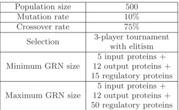
Population size 500 Mutation rate 10% Crossover rate 75%
Selection 3-player tournament with elitism 5 input proteins + Minimum GRN size 12 output proteins +
15 regulatory proteins 5 input proteins + Maximum GRN size 12 output proteins +
50 regulatory proteins Table 1: Parameters of the genetic algorithm used to train the GRN.
sub-network, and the local connectivity is maintained; only new links between the different sub-networks are created.
Mutation is applied in three equally probable ways: mu-tating an existing protein by randomly changing one of its
three integers, adding a new protein randomly generated or
removing one protein randomly chosen in the network.
The coefficients β and δ presented in the dynamics model are encoded in a second independent chromosome which contains only these values. They are coded with double-precision floats in [0.5; 2] (empirically chosen).
In this work, we have used a master-worker model dis-tributed genetic algorithm in order to reduce the optimiza-tion duraoptimiza-tion. Table 1 presents the parameters used to evolve the gene regulatory network in this experience.
As the developmental process is completely deterministic, running the developmental process only once is sufficient to calculate the fitness of the corresponding wind farm layout. However, to avoid over-specialization on one scenario, this procedure is repeated on three different scenarios and the minimum fitness of all three scenarios is kept as the final fitness. The wind scenarios used to train the regulatory net-work are described in the supplementary materials as sce-narios 1-3, and are available for download as well as part of the aforementioned open source software.
7.
COMPARATIVE STUDY
We compare Devo-II to a set of state-of-the-art layout optimization techniques: a genetic algorithm (GA), Particle
Initial state Final layout
Figure 3: Example of development of a layout, show-ing the first, middle, and last developmental steps.
Swarm Optimization (PSO), and the Turbine Distribution Algorithm (TDA). We also compare Devo-II to Devo-I. After briefly explaining these techniques, which are further detailed in [12, 20, 23], this section presents these compar-isons.
7.1
Existing approaches
7.1.1
Genetic algorithm (GA)
Genetic algorithms are commonly used to optimize wind farm layout. The farm area is discretized with a grid [15, 7, 9, 21, 6, 18, 24]. The size of each cell of the grid corresponds to the minimal security distance between 2 turbines. The genetic algorithm then optimizes a binary genome in which each gene represents the presence or absence of a turbine in each cell of the grid. This approach has the advantage of optimizing the number of turbines, but the position of the turbines is not precisely optimized as they are limited to the center of the cell. In the scope of this study, we have im-plemented our own genetic algorithm. The fitness function used to evaluate each layout is the one presented in equa-tion 2. The genetic algorithm is set up with a populaequa-tion size of 500 individuals, a 3-player tournament selection with elitism, 20% of mutation and 70% of crossover. The genetic algorithm is run for 500 generations, which is sufficient to converge.
7.1.2
Particle swarm optimization (PSO)
In the particle swarm optimization approach, a particle represents a turbine layout by a vector of N (x, y) Carte-sian coordinates, where N is the maximum number of tur-bines[22, 1, 19]. In other words, the PSO search space has 2N dimensions, N being the maximum possible number of turbines. The particle also maintains a memory of the global best position already found in a population of particles. For each iteration of the algorithm, the particles’ velocities are calculated according to their own fitness, the position of the current best solution, and nearby particles’ positions. The next positions of the particles can be immediately deduced from the velocities. A constraint-repairing algorithm, de-scribed in [19], is used to meet the security distance con-straint. In this method, starting with an initial turbine, a turbine is added to a layout at position proposed by the particle only if it is not within the security distance to any existing turbine. The PSO is run with each particle on a dif-ferent thread with a maximum of 1000 turbines, 20 particles, a neighborhood size of 3, and the fitness function 2. The con-straint reparation mechanism causes many of the turbines to not enter the layout; 1000 as a maximum was determined empirically to place 400 turbines. The PSO is run for 100 iterations or equivalently 2000 layout evaluations, which is sufficient to converge.
7.1.3
Turbine Distribution Algorithm (TDA)
TDA uses randomized modification of turbine location starting with an initial layout [20]. At each iteration, the best layout is modified by slightly modifying a randomly chosen turbine in the layout and perturbing it to move it away from its closest neighbors in order to minimize the lo-cal interferences produced by the turbines. The new layout is compared to the previous best layout using energy output. This process is repeated a sufficient number of iterations to reach an optimal layout. This approach has the advantage of
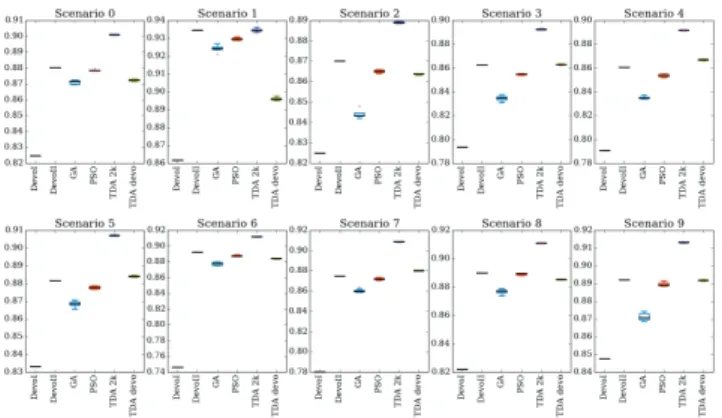
Figure 4: Results of the comparative study of layout optimization approaches. Each approach has been evaluated 8 times on each scenarios.
precisely positioning the turbines in the layout because each turbine position is computed with a high resolution but it requires a high number of layout evaluation (which is com-putationally expensive) and only works with a fixed number of turbines. This approach is, to our knowledge, the current best approach to optimize a layout with a fixed number of turbines. We have used the Wagner & al. implementation of TDA [20]2, with the number of turbines determined by
Devo-II. First, we run TDA for 2000 iterations, as done in [20], to determine an optimal layout. Then, we compare TDA running for the same number of evaluations as Devo-IIto provide a balanced comparison based on runtime.
7.1.4
Discrete developmental model (
Devo-I)
Devo-Iis very similar to Devo-II: cells are controlled by a gene regulatory network to populate a 2-D layout. They use wind velocity input to decide their action: divide, rotate their division clockwise or counterclockwise, wait and die. However, instead of populating a continuous space, the cells are confined to a grid. The size of the grid cells is equal to the security distance, which keeps the layout valid during the developmental process. The GRN is also trained with a genetic algorithm in order to produce the final layout. More details are given in [23]. The GRN has been trained with the fitness function from equation 2 on the same three training scenarios than Devo-II.7.2
Results
To evaluate Devo-II, we compare its results to layouts obtained using Devo-I, GA, PSO, and TDA on 10 different wind scenarios. Devo-I and Devo-II were exposed to 3 of the scenarios during training, but were run without exposure to the other 7. All scenarios are available in the supplemen-tary materials and online. As both Devo-I and Devo-II are deterministic once trained, the trained result was run only once on each scenario. The GA, PSO, and TDA were run 8 times on each scenario. Table 2 presents the best results for each method, and figure 4 presents the results of all runs.
First, we compare Devo-I and Devo-II. The gain brought by the use of a continuous space is undeniable. The layouts
2Since TDA also uses Kusiak’s wind model and after cross
verifications, the layouts produced by TDA produce the same energy output as the layouts produced by our imple-mentations
produced by Devo-II are 7.9% better than the discrete ones, as the use of a continuous space allows Devo-II to locally optimize the positions of the same number of turbines.
Then, Devo-II and the GA are compared. With the same fitness function, Devo-II does better on all scenar-ios: Devo-II uses more turbines but has a more efficient layout, getting a higher wake free ratio. Moreover, the num-ber of evaluations is extremely low: 250,000 evaluations for the genetic algorithm in comparison to less than 100 evalu-ations for Devo-II. The PSO again displays the advantages of a continuous model when compared to the GA, where it achieves better efficiencies with at least the same number of turbines. However, most likely due to constraint repairing mechanism [19], the PSO doesn’t perform as well as Devo-II or TDA. The number of evaluations necessary for the PSO, 2000, is very costly compared to Devo-II.
Compared to TDA with 2000 evalutions (TDA 2k), Devo-II produces solutions with a lower quality: the wake free ratio is 2.79% lower for Devo-II. However, Devo-II also optimizes the number of turbines, which is simply reused by TDA to optimize the layout.
To compare Devo-II to TDA with comparable evaluation conditions, we run TDA with the number of evaluations used by Devo-II. As shown in the column named “TDA devo” in table 2, Devo-II produces equivalent solutions in quality to TDA using the number of turbines optimized and the number of evaluations used by Devo-II.
We use a t-test to compare the results of each method with all others for each scenario. In these t-tests, only two from different methods have p > 0.05: in scenario 1, Devo-IIand TDA 2k aren’t significantly different, and in scenario 3, Devo-II and TDA devo aren’t significantly different. The t-test was performed over all 8 trials of each approach, where 2 only shows the best result from each trial.
These experiments demonstrate that Devo-II produces layouts that can compete with TDA in comparable condi-tions and outperforms GA and PSO. Moreover, Devo-II can tackle a more complex problem than TDA: the optimization of both the number of turbines and their layout. This prop-erty can be useful in the design process of wind farms. In the conclusion, we will discuss the benefits and drawbacks of this approach in the wind farm design process.
8.
ADAPTATION TO THE ENVIRONMENT
In our previous work using a discrete developmental model, Devo-I, to produce the wind farm layouts [23], we briefly show that Devo-I was able to adapt to changes in the lay-out size and to obstacles withlay-out retraining. Here, we offer a detailed study of Devo-II’s ability to adapt to changes in the layout size and to obstacles.
8.1
Adaptation to the layout size
To show the capacity of Devo-II to adapt to the layout size, we produce layouts based on the previous wind scenar-ios but on a small layout (6.2km by 9.61km) and a large one (9.92km by 20.15km). Devo-II is compared to Devo-I and TDA with 2000 evaluations. Table 3 shows the results of this study. Both Devo-I and Devo-II’s results are de-terministic, and TDA was run 8 times and the maximum fitness is showed in the table. As in the comparative study, TDA is run with the number of turbines given by Devo-II. The same conclusion as in §7 can be made when compar-ing these approaches, Devo-I, Devo-II, and TDA, on the
Scenario Devo-II Devo-I GA PSO TDA 2k TDA devo Rwf #t #e Rwf #t #e Rwf #t #e Rwf #t #e Rwf #t #e Rwf #t #e 0 0.880 403 100 0.825 399 100 0.873 399 250k 0.880 400 2000 0.901 403 2000 0.873 403 100 1 0.934 408 100 0.862 461 100 0.927 400 250k 0.928 400 2000 0.936 408 2000 0.898 408 100 2 0.870 400 100 0.825 406 100 0.858 400 250k 0.865 405 2000 0.890 400 2000 0.864 400 100 3 0.857 400 59 0.794 405 100 0.838 400 250k 0.855 401 2000 0.892 400 2000 0.863 400 59 4 0.853 399 58 0.791 466 100 0.837 399 250k 0.851 398 2000 0.893 399 2000 0.863 399 58 5 0.881 405 100 0.833 403 100 0.871 399 250k 0.879 404 2000 0.908 405 2000 0.885 405 100 6 0.892 400 100 0.781 627 100 0.880 400 250k 0.890 402 2000 0.912 400 2000 0.886 400 100 7 0.875 402 61 0.780 479 100 0.879 400 250k 0.871 404 2000 0.909 402 2000 0.881 402 61 8 0.890 409 62 0.822 523 100 0.879 400 250k 0.889 404 2000 0.911 409 2000 0.886 409 62 9 0.891 401 57 0.848 424 100 0.874 400 250k 0.889 404 2000 0.913 401 2000 0.892 401 57
Table 2: Maximum results of the comparative study of the wind farm layout optimization approaches. Italic values represents the parameters given to the algorithm, and thus not optimized. Columns are the wake free ratioRwf , the number of turbines #t and the number of layout evaluation #e required to produce the
layout.
small and large layouts: TDA achieves optimal results but of the same order of magnitude (on average, TDA is 2.76% better than Devo-II). This means Devo-II scales perfectly when the environment configuration changes; it performs the same relative to TDA as it does on the training layout. The number of evaluations is particularly crucial in this ex-periment, in particular on large layouts; whereas Devo-II needs less than 4 minutes to produce the layouts, TDA 2k needs nearly one hour for each layout.
8.2
Handling obstacles
Devo-II can naturally handle obstacles in the environ-ment. This property is crucial since the wind farm design process has to account for possible obstacles such as lakes, roads, buildings, etc. In our approach, an obstacle is de-signed as a invalid position where the cells are forbidden to
Sc Size Devo-II Devo-I TDA 2k Rwf #t #e Rwf #t #e Rwf #t #e 0 small 0.884 248 61 0.817 275 61 0.907 248 2000 1 small 0.940 244 61 0.845 345 61 0.945 244 2000 2 small 0.871 245 41 0.804 275 61 0.897 245 2000 3 small 0.868 242 47 0.796 291 61 0.900 242 2000 4 small 0.857 254 43 0.830 230 61 0.893 254 2000 5 small 0.887 246 61 0.799 345 61 0.914 246 2000 6 small 0.895 248 61 0.772 256 61 0.916 248 2000 7 small 0.878 245 45 0.733 351 61 0.916 245 2000 8 small 0.896 246 52 0.848 254 61 0.918 246 2000 9 small 0.894 247 41 0.813 335 61 0.918 247 2000 0 large 0.879 817 205 0.813 1013 205 0.890 817 2000 1 large 0.922 833 205 0.865 1012 205 0.924 833 2000 2 large 0.860 824 205 0.796 936 205 0.876 824 2000 3 large 0.849 817 79 0.784 1012 205 0.881 817 2000 4 large 0.847 841 87 0.808 786 205 0.876 841 2000 5 large 0.878 817 87 0.817 1013 205 0.898 817 2000 6 large 0.887 824 87 0.743 1013 205 0.900 824 2000 7 large 0.869 819 81 0.793 1010 205 0.898 819 2000 8 large 0.886 814 81 0.837 900 205 0.903 814 2000 9 large 0.879 863 205 0.830 858 205 0.899 863 2000 Table 3: Results of the modification of the farm size. Italic values represent the parameters given to the algorithm, and thus not optimized.
Scenario
No obstacle Obstacles Size Energy # of Size Energy # of (km2) per km2 turb. (km2) per km2 turb.
0 98 26,474 403 96.04 28,966 401 1 98 54,640 408 96.04 54,813 402 2 98 19,546 400 96.04 20,253 409 3 98 24,506 400 96.04 25,241 404 4 98 22,064 399 96.04 22,561 399 5 98 32,333 405 96.04 32,558 399 6 98 36,727 400 96.04 38,547 417 7 98 32,730 402 96.04 32,542 391 8 98 37,553 409 96.04 37,240 398 9 98 38,460 401 96.04 39,573 406 Table 4: Obstacle handling with Devo-II
go. Here again, no further training is necessary to take this new constraint into consideration: the evolved GRNs can directly produce layouts optimized with the obstacles.
To our knowledge, Devo-I and Devo-II are the only ap-proaches that currently tackle this problem. Therefore, to evaluate the quality of the generated layout, we propose a comparison of the energy output per kilometer square avail-able in the environment. We use an initial 7km x 14 km layout size in this study. Table 4 presents the results of this comparison.
The energy per km2is very comparable between the layout
with and without obstacles. It only differs 2.4% on average on the 10 scenarios. This comparison is conclusive: Devo-IIcan adapt to obstacles in environment without modifying the properties of the layout it generates.
9.
CONCLUSION
The paper presents a continuous developmental model, Devo-II, to optimize wind farm layouts. To evaluate this novel approach, we compare it to state-of-the-art techniques in layout optimization. We show that, in comparable con-ditions, Devo-II generates layouts with comparable quality to those from state-of-the-art techniques. However, Devo-II optimizes both the number of turbines and their layout, and can adapt to handle changing layout size and obstacles without retraining. These properties are crucial during the design process of a wind farm.
The main benefit of this approach is its immediate reac-tivity which is not found in other approaches. The devel-opmental model only needs a few seconds to adapt to new constraints. Therefore, Devo-II could be an helpful tool for wind farm designers, bearing in mind that the layout process requires a great deal of auxillary input guidance from engi-neers. Devo-II could be used as a real-time optimization tool during this design phase. Designers could interact with the cells, constraints, etc. while the cells are optimizing the layout.
Of course, because Devo-II doesn’t currently provide the optimal layout, this tool could be used along with a stan-dard layout optimizer. TDA could be used, for example, to precisely position the final turbines generated by Devo-II. Our hypothesis is that TDA could optimize this layout faster and potentially better because of Devo-II, which provides the number of turbines and an efficient starting layout.
Acknowledgement
This work was granted access to the HPC resources of CALMIP under the allocation 2013-1319
10.
REFERENCES
[1] S. Chowdhury, J. Zhang, A. Messac, and L. Castillo. Unrestricted wind farm layout optimization (uwflo): Investigating key factors influencing the maximum power generation. Renewable Energy, 38(1):16–30, 2012.
[2] S. Cussat-Blanc, J. Pascalie, S. Mazac, H. Luga, and Y. Duthen. A synthesis of the Cell2Organ
developmental model. Morphogenetic Engineering, 2012.
[3] S. Cussat-Blanc, S. Sanchez, and Y. Duthen. Controlling cooperative and conflicting continuous actions with a gene regulatory network. In Conference
on Computational Intelligence in Games (CIG’12).
IEEE, 2012.
[4] E. H. Davidson. The regulatory genome: gene regulatory networks in development and evolution.
Academic Press, 2006.
[5] R. Doursat. Organically grown architectures: Creating decentralized, autonomous systems by embryomorphic engineering. Organic Computing, pages 167–200, 2008. [6] A. Emami and P. Noghreh. New approach on
optimization in placement of wind turbines within wind farm by genetic algorithms. Renewable Energy, 35(7):1559–1564, 2010.
[7] S. Grady, M. Hussaini, and M. M. Abdullah. Placement of wind turbines using genetic algorithms.
Renewable Energy, 30(2):259–270, 2005.
[8] P. E. Hotz. Genome-physics interaction as a new concept to reduce the number of genetic parameters in artificial evolution. In Evolutionary Computation,
2003. CEC’03. The 2003 Congress on, volume 1,
pages 191–198. IEEE, 2003.
[9] H.-S. Huang. Distributed genetic algorithm for optimization of wind farm annual profits. In
Intelligent Systems Applications to Power Systems, 2007. ISAP 2007. International Conference on, pages
1–6. IEEE, 2007.
[10] M. Joachimczak and B. Wr´obel. Evo-devo in silico: a model of a gene network regulating multicellular
development in 3d space with artificial physics. In
Proceedings of the 11th International Conference on Artificial Life, pages 297–304. MIT Press, 2008.
[11] M. Joachimczak and B. Wr´obel. Evolving Gene Regulatory Networks for Real Time Control of Foraging Behaviours. In Proceedings of the 12th
International Conference on Artificial Life, 2010.
[12] S. A. Khan and S. Rehman. Iterative
non-deterministic algorithms in on-shore wind farm design: A brief survey. Renewable and Sustainable
Energy Reviews, 19:370–384, 2013.
[13] V. Komkov. Optimal control theory for the damping of
vibrations of simple elastic systems. Springer-Verlag
Berlin, 1972.
[14] A. Kusiak and Z. Song. Design of wind farm layout for maximum wind energy capture. Renewable Energy, 35(3):685–694, 2010.
[15] G. Mosetti, C. Poloni, and B. Diviacco. Optimization of wind turbine positioning in large windfarms by means of a genetic algorithm. Journal of Wind
Engineering and Industrial Aerodynamics,
51(1):105–116, 1994.
[16] M. Nicolau, M. Schoenauer, and W. Banzhaf. Evolving genes to balance a pole. Genetic
Programming, pages 196–207, 2010.
[17] B. Porter. A developmental system for organic form synthesis. In Artificial Life: Borrowing from Biology, pages 136–148. Springer, 2009.
[18] S. ¸Si¸sbot, ¨O. Turgut, M. Tun¸c, and ¨U. ¸Camdalı. Optimal positioning of wind turbines on g¨ok¸ceada using multi-objective genetic algorithm. Wind Energy, 13(4):297–306, 2010.
[19] K. Veeramachaneni, M. Wagner, U.-M. O’Reilly, and F. Neumann. Optimizing energy output and layout costs for large wind farms using particle swarm optimization. In Evolutionary Computation (CEC),
2012 IEEE Congress on, pages 1–7. IEEE, 2012.
[20] M. Wagner, J. Day, and F. Neumann. A fast and effective local search algorithm for optimizing the placement of wind turbines. Renewable Energy, 51(0):64 – 70, 2013.
[21] C. Wan, J. Wang, G. Yang, X. Li, and X. Zhang. Optimal micro-siting of wind turbines by genetic algorithms based on improved wind and turbine models. In Decision and Control, 2009 held jointly
with the 2009 28th Chinese Control Conference. CDC/CCC 2009. Proceedings of the 48th IEEE Conference on, pages 5092–5096. IEEE, 2009.
[22] C. Wan, J. Wang, G. Yang, and X. Zhang. Optimal micro-siting of wind farms by particle swarm
optimization. In Advances in swarm intelligence, pages 198–205. Springer, 2010.
[23] D. Wilson, E. Awa, S. Cussat-Blanc,
K. Veeramachaneni, and U.-M. O’Reilly. On learning to generate wind farm layouts. In Proceeding of the
fifteenth annual conference on Genetic and evolutionary computation conference. ACM, 2013.
[24] C. Xu, Y. Yan, D. Y. Liu, Y. Zheng, and C. Q. Li. Optimization of wind farm micro sitting based on genetic algorithm. Advanced Materials Research, 347:3545–3550, 2012.