The alpha of a market timer

The Performance of a Market Timer

Georges HÜBNERy

April 2012

Abstract

The Treynor and Mazuy framework is a widely used return-based model of market timing, but existing corrections of the regression intercept can be manipulated through derivatives trading. We propose an adjustment based on Merton’s option replication approach. The linear and quadratic coe¢ cients of the regression are exploited to assess the cost of the replicating option that yields similar convexity for a passive portfolio. A similar reasoning applies for various timing patterns and in multi-factor models. Our empirical application shows that, unlike existing performance adjustment methods, the portfolio replication approach uncovers a positive link between the convexity and the performance of market timing funds.

Keywords: Performance measurement, market timing, Treynor and Mazuy, option replica-tion, mutual fund performance.

JEL codes: G10, G12

This paper has bene…ted from comments by Hatem Ben Ameur, Maria Ceu Cortez, Georges Gallais-Hamonno, Marie Lambert, Bertrand Maillet, Guillaume Monarcha, Hery Raza…tombo, as well as the Workshop on Investment Funds at University of Luxembourg, the Thematic Cluster Day on Hedge Funds of the University of Orleans, the 2011 French Finance Association Conference (Montpellier), and the 2011 European Financial Management Association Annual Meeting (Braga) attendees. I thank Thomas Lejeune and Arnaud Cavé for excellent research assistance. Financial support from Deloitte Belgium and Deloitte Luxembourg is gratefully acknowledged. All errors remaining of mine.

y_{Deloitte Chaired Professor of Portfolio Management and Performance, HEC Management School - University}

of Liège, Belgium; Associate Professor, School of Economics and Business, Maastricht University, the Netherlands; Founder & Chief Scienti…c O¢ cer, Gambit Financial Solutions Ltd, Belgium. Corresponding address. University of Liège, HEC Management School, Rue Louvrex 14 - N1, B-4000 Liège, Belgium. Phone: (+32) 42327428. E-mail: [email protected]

1

Introduction

Assessing the performance of actively managed funds is an ongoing theoretical and empirical chal-lenge. According to the hypothesis of e¢ cient …nancial markets, active fund managers should not take advantage of proprietary skills that would generate reproducible positive abnormal returns. For that purpose, traditional performance measures such as the Sharpe (1966) ratio, Jensen’s (1968) alpha as well as the Treynor (1965) ratio, and the information ratio, respectively controlling for total, systematic and speci…c risks, are designed to capture performance of portfolios delivering stationary returns in a mean-variance environment. These measurement approaches re‡ect a clear aim to detect the manager’s ability to perform superior asset selection. When several risk factors are identi…ed, these measures all bear a multi-factor extension, and the task of performance mea-surement remains little controversial. Measures derived from Jensen’s alpha have been extensively used in this context, as evidenced in the comprehensive study by Kothari and Warner (2001). But when a fund’s observed returns follow an unstable pattern, a fundamental question arises: is this due to non-linear risk exposures, or does it result from voluntary variations of the manager’s betas re‡ecting some kind of market timing skills?

In the context of hedge funds returns, whose frequencies are usually monthly, the vast majority of the literature has responded a¢ rmatively to the former branch of the alternative (see Fung and Hsieh, 2001; Agarwal and Naik, 2004). Only few recent papers (Chen and Liang, 2007; Detemple et al., 2010) explicitly associate hedge funds’time-varying betas to a potential market timing behavior. In the mutual fund literature, the performance measurement literature has mostly taken the other direction: changing betas indicate market timing. The alternative explanation, which attributes risk shifting to the use of derivatives as a way to curb risk exposures, does not correspond to empirical evidence (Koski and Ponti¤, 1999): most mutual fund managers who use derivatives seem to use them to stabilize their risk exposures Two reasons explain this divergence. First, a benchmark can generally be identi…ed. It either leads the speci…cation of a control portfolio, or to regression-based procedures for the estimation of required portfolio returns. Portfolio managers claim to be able to generate returns above their benchmark through superior selectivity of securities or asset classes (asset selection), or by successfully anticipating market movements (market timing). Second, returns are observable with a higher frequency (daily or weekly), and this eases the uncovering of a return di¤erential associated to variations in risk exposures or, even more precisely, in portfolio holdings.

To date, two return-based approaches have been used on a regular basis for the detection of market timing skills: the piecewise linear regression of Henriksson and Merton (1981) (henceforth HM) and the quadratic regression of Treynor and Mazuy (1966) (henceforth TM).1 Empirical

idence based on these measures have regularly delivered a disappointing picture regarding market timing skills (see a.o. Kryzanowski et al., 1996; Becker et al., 1999; Bollen and Busse, 2004; Comer et al., 2009). Beyond con…rming such evidence, Krimm et al. (2011) also …nd out a negative rela-tionship between timing and global performance. However, a direct holding-based approach delivers a more equivocal picture. Kaplan and Sensoy (2008) …nd evidence of a positive relationship between variations of equity betas and market returns for market timing funds. In their study of detailed portfolio holdings, Jiang et al. (2007) concludes that the average performance attributable to tim-ing skills is positive, and could amount up to an annual 0.6%. The extent of this abnormal return is economically relevant but the contrast of this result with pervasive evidence is also empirically puzzling. Elton et al. (2011), through a more granular analysis of holdings, conclude that most of the outperformance fades away when using a multi-index model. Even though they outline that market timing exists as well, they …nd out an average underperformance of market timers, mostly because of the managers with the most negative market timing behavior. A potential explanation could be provided by Huang et al. (2011), who show that risk-shifting of mutual funds portfolio holdings could be largely attributable to unskilled or agency-proned managers. These managers tend to increase risk at wrong times, leading to negative convexity in portfolio returns.

Reconciling the performance delivered by a simple model like HM or TM with the one retrieved from a holding-based model is a more arduous task than merely comparing alphas, even when the econometrics are carefully executed. Ingersoll et al. (2007) demonstrate how easily one can manipulate all performance measures listed above, included alphas, by altering the distribution of returns, or by dynamically trading securities to curb the distribution of returns. Such option-like characteristics displayed by the pattern of portfolio returns has long been explicitly associated with spurious market timing e¤ects (Jagannathan and Korajczyk, 1986). The mere separation between the regression intercept and the market timing coe¢ cient in the HM and the TM models is not su¢ cient to discriminate between genuine and false market timing skills. For instance, Lee and Rahman (1990) separate asset selection and market timing by considering that the alpha fully represents the former dimension. To better identify pure market timers, three types of adjustments of alphas have been proposed: a variance correction approach (Grinblatt and Titman, 1994); an approximation based on the squared benchmark returns (Bollen and Busse, 2004); and a synthetic option pricing approach (Merton, 1981). All three methods, however, remain prone to manipulations because a manager who has access to a complete derivatives market can easily alter the timing coe¢ cient without a¤ecting the regression intercept (alpha) to a proportional extent. Based on this statement, Ingersoll et al. (2007) propose a manipulation-proof performance measure, but its identi…cation is contingent on the characterization of the investor’s preferences.

In this paper, we revisit the Treynor and Mazuy model by applying, almost literally, the original option replication approach proposed by Merton in the context of the HM model. Unlike all previous attempts to alter the TM regression alpha on the basis of the quadratic term alone, we exploit information on both the linear and the quadratic coe¢ cients of the regression to assess the replicating cost of the option for a passively managed portfolio with non-linear benchmark exposures. The intuition goes as follows. If the manager has free access to a complete derivatives market on its benchmark, as indicated by Ingersoll et al. (2007), she can indeed curb the payo¤ of her portfolio in many possible ways. Considering the benchmark case where asset return distributions are stationary and Gaussian, one can always approximate the returns of the option portfolio up to the second (quadratic) order through a Taylor series expansion. Then, only the option delta, gamma and theta matter. Anyone can mix these option "greeks" to get the desired linear and quadratic sensitivities, but the same greeks will also entirely drive the periodic holding cost of this portfolio. Amongst all portfolios involving derivatives that mimic a fund’s pattern of returns, the cheapest one provides the minimum performance required from a manager who claims to time the market. The actual performance of the active fund, mixing the impact of asset selection and market timing skills, is obtained by di¤erence. To illustrate our approach, we show that existing market timing performance measures could mistakenly assign nonzero performance to a pure passive fund involving options, while our correction properly sets the adjusted performance of an uninformed portfolio to zero.

This approach has the potential to overcome the performance manipulation issue. We derive a proper performance adjustment in a preference-free setup or, more precisely, in an economy where preferences are consistent with mean-variance analysis. The availability of a complete market enables us to carry out an arbitrage argument, unlike in Ingersoll et al. (2007) whose correction involves replicating a non-traded option on the quadratic market return, resulting in market incompleteness. The practical application of our approach involves the delicate choice of the replicating option maturity. We create a portfolio whose quadratic sensitivity to the benchmark returns reproduces the pattern of the TM regression. But both equations involve a noise component: the speci…ca-tion error in the TM regression, and the approximaspeci…ca-tion error in the Taylor series expansion of the replicating portfolio. The former error can be reduced by extending the reasoning to a multivariate setup, with the advantage that one does not need to identify interaction terms as in the extension of the TM model proposed by Lehmann and Modest (1987). The latter issue is more tricky, because the sign and magnitude of the error cannot be determined a priori. Furthermore, the quest for the cheapest-to-replicate option might lead to situations where the cheapest option displays unaccept-able approximation errors. We carry out an experiment on the U.S. market. The results suggest that the choice of option maturing in 6 months provide a reasonable trade-o¤ between approximation error and replication cost when returns are measures on a weekly interval.

The empirical application of the new correction delivers particularly encouraging results. From a basis of 1,262 equity mutual funds, we study two subsamples of funds with positive and negative convexity of their market sensitivity, respectively. If market timing skills exist, one would expect the performance of convex portfolios to increase with their convexity level. Concave funds that volun-tarily adopt a contrarian stance might deliver superior performance to compensate for their gamma risk, but one would expect the emphasis of market timing skills to be much less pronounced because of the spurious e¤ect induced by positive cash in‡ows when markets are up, which mechanically reduce the fund’s beta (Warther, 1995; Edelen, 1999). The application of the option portfolio repli-cation approach yields the predicted pattern of results. All other attempts to correct the TM model with existing adjustment methods fail to a signi…cant extent. They underestimate the necessary correction for the fund’s convexity, leaving positive timers with negative adjusted performance and vice-versa. This bias explains the converging conclusion of most studies based on the TM model that market timers do not outperform the market. Besides the issue of their biased level, inadequate corrections appear to weaken the link between the magnitude of market timing and the associated performance. Such results suggest that a correction of alpha based on an arbitrage argument clari-…es the role of market timing in the generation of performance. This will undoubtedly improve the diagnostics regarding the market timing skills of portfolio managers.

The paper is organized as follows. The second section introduces the alternative approaches to account for market timing in performance evaluation, including the option replicating portfolio correction proposed in this paper. In section 3, we discuss the adjustments necessary to cope with estimation or approximation issues, and deliver associated potential solutions. Section 4 presents the results of an empirical study on a sample of mutual funds, with which the impacts of alternative adjustment methods are tested. Section 5 concludes.

2

The option-based approach to market timing

In the scope of the one-factor model for asset returns, the literature identi…es two major speci…ca-tions allowing to expose a manager’s market timing abilities. The Henriksson and Merton (1981) model considers that the manager switches the portfolio’s beta depending on the sign of the market return. A good market timer increases the market exposure when the return is positive, and keeps it lower otherwise. Treynor and Mazuy (1966) propose to add a quadratic term to the one-factor model. The coe¢ cient of this term re‡ects the convexity achieved by the manager in her exposure to the market portfolio. If it is positive, the manager gradually increases her beta as the market goes up, indicating that she displays good timing abilities. The regression equations of the Henriksson and Merton (1981) and the Treynor and Mazuy (1966) models are represented in equations (1) and

(2), respectively:

rt= HM + HMrmt+ HM r+mt + "t (1)

rt= TM+ TMrmt+ TMr2mt+ "t (2)

where rt Rt Rf is the portfolio excess return over the risk-free rate, rmtis the market portfolio

excess return, and r+_mt= max ( rmt; 0).

The HM model translates the behavior of a manager who succeeds in switching her market beta from a high level equal to _HM when the market return exceeds the risk-free rate to a low level of ( _{HM HM}) otherwise. Admati et al. (1986) show that under the standard assumption of a joint normal distribution of asset returns, the TM model is consistent with a manager whose target beta varies linearly with her forecast for the expected market rate of return. In both models, a negative value of gamma induces negative market timing.

The literature has proposed many extensions of these two models in the context of multiple risk factors or benchmark portfolios2_{, but so far there has been no widely adopted alternative approach}

to market timing performance evaluation under a single factor speci…cation.

2.1 The classical view of performance as an additive measure

The HM model and the TM models aim to capture timing and selectivity skills using one single equation. Under both speci…cations, the constant of the regression is supposed to capture the asset selection skills of the manager. The coe¢ cient of the second variable (the truncated positive market return for HM and the squared market return for TM) reveals her ability to time the market, but it does not deliver a measure of excess return due to market timing by itself. So far, the literature on mutual fund performance has produced three alternative ways to measure the contribution of market timing to active returns: one based on the variance of market returns, another one of the squared market returns, and a …nal one based on the value of an option.

The work of Admati et al. (1986) characterizes the properties of an active market timing portfolio managed optimally if returns are multivariate normal and the representative investor exhibits a constant absolute risk aversion (CARA) utility function. It is assumed that the manager, when receiving information about market returns, linearly adjusts her beta to the timing signal. They show that the optimal portfolio returns are characterized by a quadratic function that can be measured by equation (2). In this particular instance of the TM model, the reward for the manager’s market timing ability is adequately represented by the variance of the market portfolio returns (Grinblatt and Titman, 1994), leading to equation (3) for the total return attributable to

2_{See Pesaran and Timmermann (1994) for the HM model, and Bollen and Busse (2001, 2004), Comer}

the manager’s performance, denoted :

TM,v= TM+ TM 2m (3)

where 2

m is the variance of the market portfolio returns.

Coles et al. (2006) and derive the corresponding formulation for the performance return in the HM model:

HM,v = HM+ HM r+m frm>0rm (4)

where r+_m = _T1 max (rmt; 0) and frm>0 denotes the frequency of positive market returns.

3

In the framework of Admati et al. (1986), the identi…cation market timing premium is a step towards the identi…cation of the coe¢ cients of the regression, which corresponds to the optimal tim-ing portfolio when the portfolio manager makes linear beta adjustments to timtim-ing signals (Grinblatt and Titman, 1994). This framework is thus restrictive. It entails an analytical connection between the regression coe¢ cients TM and TM in equation (2). Detemple et al. (2010) characterize further

this connection by deriving a continuous-time generalization of market timing models, encompass-ing HM and TM as special cases. They derive a closed-form solution for the correlation structure between the fund’s and the market returns, and adapt equations (4) and (3) accordingly. For the TM model, the total performance adjusted for time-varying correlations collapses to expression (3) divided by the volatility of the portfolio returns.

A simpler approach is proposed by Bollen and Busse (2004) and Comer et al. (2009). They build upon the fact that, in the HM and TM model, a perfect market timer ex post would make her beta time-varying according to market conditions by setting, respectively, _HM;t = _HM1_frm;t>0g and _TM;t = _TM + _TMrm;t. Accordingly, the total performance of a manager combining asset

selection and market timing skills results from averaging the periodic market returns in the model with time-varying betas:

HM,a= HM+ HMrm+ (5)

TM,a = TM+ TMr2m (6)

Equations (5) and (6) are simpli…ed versions of (4) and (3), respectively. The advantage of this formulation is that it is no longer restricted to correspond to an optimal behavior as in the Admati et al. (1986) framework, but the cost is a potentially high upward bias in the performance as measured with these metrics. When returns are computed with a daily frequency, the di¤erence between the corresponding equations does not appear to matter empirically (Krimm et al., 2011). However, as

3

The authors transform the original HM model by estimating the regression rt = HM + HMrmt+ HMr+mt+ "t, but the outcome remains the same regarding the determination of the manager’s total perfor-mance.

the expected market return becomes signi…cant with longer measurement intervals, the upward bias in equations (5) and (6) may start to matter.

All three formulations for share a common additive structure. They leave the una¤ected, considering it as the contribution of selectivity to performance. The market timing coe¢ cient mul-tiplied by a premium constitute the second term of the sum. Note that the market beta does not intervene explicitly in the formula. In the Admati et al. (1986) approach, this coe¢ cient represents an output of the model. It does not appear in the empirical approach of Bollen and Busse (2004) either.

In the next section, we defend an alternative approach that explicitly accounts for the role of the linear market beta in total performance with market timing. As for the original option-based approach proposed by Merton (1981), we associate the market timing return to an option. Our analysis focuses on the cost, expressed in returns, of replicating the pattern of the HM or TM regression using a mix of options and risk-free instruments only.

2.2 The replicating cost of building market timing portfolios

Both the Admati et al. (1986) and the Bollen and Busse (2004) frameworks use an ex post approach to the detection of market timing. They aim at directly measuring the contribution of market timing skills in the total portfolio return, irrespective of how the manager tried to achieve this result. When considered ex ante, the skill of the manager is related to her capacity to create an option on the market portfolio.

2.2.1 The Henriksson and Merton model reinterpreted

The idea of calling upon option trading strategies to assess the market timing abilities of a portfolio manager is introduced by Merton (1981). In the context of the HM model –developed in his sequel paper coauthored with Henriksson – he shows that the portfolio manager’s global performance, combining her timing and selectivity abilities, expressed in realized returns and denoted , can be represented as

HM,o = HM + HMeRf tP M; t; eRf t (7)

where P M; t; eRf t _{is a put with remaining time to maturity equal to the time interval and}

strike price of eRf t_{written on the market portfolio M , whose price is normalized to 1}

The reasoning underlying Merton’s result is that the portfolio return obtained in equation (1) can be achieved by taking at the same time a long position of _HM in the underlying index and of

HM in a put on the same index that will only pay o¤ if the index return is lower than the riskless

the risk-free rate. The cost of adopting such a strategy is the initial put premium, which is a lump sum amount P S; t; eRf t _{per unit of gamma, and that should be capitalized to represent the}

realized opportunity cost of the strategy versus a linear one. Ingersoll et al. (2007) adapt (7) to the TM framework and get

TM,o = TM+ TMe2Rf t e

2

m t _{1 (8)}

where Rf is the continuous interest rate and 2m is the volatility of the market portfolio returns.

The authors interpret the second term of this expression as the payo¤ for the fraction _TM of a derivative security that pays the square of the excess market return. At the same time, Ingersoll et al. (2007) emphasize that this de…nition of total performance is easily prone to manipulation.

There are two major di¤erences between the original Merton (1981) interpretation of the HM model and the transformation proposed by Ingersoll et al. (2007). The …rst one is that, once we depart from the Admati et al. (1986) strict optimization framework, the value of _TM in the TM formulation can be fully independent of the level of _TM. A market timer can freely choose her beta and, at the same time, achieve a level of performance that depends on her skill (or luck) in timing the market. In the HM model, this is not so: the level of _HM re‡ects the di¤erence between the high market beta and the low market beta. Therefore the value of _HM is present, although implicitly, in equation (7). The second reason for the di¤erence is that the Merton interpretation rests on the cost of replicating a protective put on the market. The quadratic option proposed in equation (8) is not tradable, and so the reasoning is held in a context of incomplete markets. Below, we follow the very same reasoning as Merton (1981) under the scope of the TM model.

2.2.2 The Treynor and Mazuy model revisited

Following the idea of Ingersoll et al. (2007), we examine the properties of a passive portfolio strategy that would exhibit a pattern of returns similar to equation (2). In the absence of any managerial skill, there is a direct connection between the levels of beta and gamma coe¢ cients on the one side, and the intercept of the regression on the other side. The di¤erence between the resulting "passive" level of alpha and the actual alpha delivers the performance attributable to the manager.

Consider a simple self-…nancing investment strategy consisting in creating a long position in an index with a positive or a negative convexity in returns and lending or borrowing at the risk-free rate. A position involving a long call option written on this index has a positive delta and a positive gamma. Similarly, a position involving a short put option has a positive delta and a negative gamma. In principle, one can …nd an option whose time-to-maturity and moneyness match the desired sensitivities to the underlying index.

Formally, rewrite equation (2) of the actively managed portfolio to replicate in terms of total returns:

Rt Rf = TM + TM(Rmt Rf) + TM(Rmt Rf)2+ "t

) Rt' 0TM+ TMRmt+ TMR2mt+ "t (9)

where 0_TM = TM+ (1 TM) Rf and the second line follows from that R2f ' 0 and RmtRf ' 0.

To reproduce the pattern of (9) with a positive convexity, we create a passive portfolio consisting in a long position w > 0 in a call option on the market index, the remainder of the portfolio (1 w) being held in the risk-free asset. Unlike in the HM model, in which the maturity and moneyness of the option are constrained by the return generating function, the option characteristics are left open. As before, we normalize to 1 the price of the market portfolio at time t.

Using the second order Taylor series expansion, the rate of return during the interval t of the portfolio can be expressed using the "greeks", i.e. the partial derivatives of the call with respect to selected variables: R( ; )_t = w ; Rmt+ 1 2 ; R 2 mt+ ; + (1 w) Rf + o( t) (10)

where and are the time-to-maturity and the strike price (expressed as a multiple of the spot price) of the option, respectively, and ; @C(M; ; )_@M , ; @

2_{C(M; ; )}

@M2 and ; @C(M; ; )_@t

are the option delta, gamma and theta. Note that, in the context of constant interest rates and market volatility over the time interval, the remaining greeks (rho and vega) do not show up. The remaining term o( t) results from the higher orders of the Taylor series expansion and from the potential rho and vega e¤ects.

Besides the residual term, equations (9) and (10) look very similar. The linear and quadratic coe¢ cients are equal if the following set of conditions is satis…ed:

TM = w ; (11)

TM = w

1

2 ; (12)

In general, the system of two equations with three unknowns ; , ; and w is inde…nite,

as there exists a continuum of pairs ( ; ) that satisfy conditions (11) and (12). Nevertheless, as this portfolio is a passive one, the objective of this replicating portfolio is to minimize the cost of replication, i.e. to maximize the constant rate of return, that we call ( ; ) = w ; ; +

(1 w ; ) Rf. The solution of this problem is given through the following program:

( ; ) _{= max} ; (w ; ; + (1 w ; ) Rf) (13) s.t. 2 ; ; = TM TM (14)

where w ; T M_; > TM.

Knowing portfolio coe¢ cients _TM and _TM, one has to screen all index call options that respect equation (14). For each eligible pair ( ; ), there is a corresponding weighting coe¢ cient w ; that

allows a check of equation (13). The optimal pair ; is obtained by screening all possible matu-rities, getting the corresponding moneyness, and verifying the values of ( ; )_{to get the maximum}

one.

To obtain the excess performance of the active portfolio that yields the returns (9) over the replicating portfolio, we deduct ( ; ):

TM = 0TM ( ; ) = TM+ (w ; TM) Rf w ; ; (15) = TM+ TM 1 ; 1 Rf ; ; (16) As w ; > TM and ; < 0 (Merton, 1981), both terms between brackets are positive. The

…rst term re‡ects the interest income saved by the portfolio manager over the replication portfolio. It represents the incremental money market return earned over the passive portfolio, which has to invest in options a higher proportion of the portfolio than the original exposure to the market index. The second term features the option theta, as in Merton (1981). It simply translated the loss in the option time value consecutive to the passage of time. Because the adjustment for market timing is strictly positive, a passive manager who generates no performance must generate a negative regression intercept TM.

2.2.3 Interaction of directional and quadratic exposures

The reasoning underlying the option replication approach can naturally be extended to the cases of negative convexity and/or of negative directional exposure.

The situation of a portfolio manager who negatively times the market involves a negative con-vexity coe¢ cient _TM < 0 (where index TM means negative market timer). The analysis is then conducted along a similar line as above. The replicating portfolio involves going short an amount of w puts on the index and investing 1 + w in the riskless asset. The performance of the "contrarian" market timer, denoted _TM, is obtained by the following equation:

TM = TM w ; + TM Rf + w ; ; (17)

The second and third term are both negative. The intercept of the regression corresponding to a neutral performance is positive.

A manager who adopts a negative directional exposure, such as a Short Selling fund, also …ts in this framework. To replicate a fund with a negative beta and a positive gamma, one has to use

a long position in a put option. If both the portfolio beta and gamma are negative, then a short position in a call option will be adopted.

The situation of a market neutral fund cannot be replicated by a simple strategy involving a call or a put. Indeed, to create an option portfolio with zero (or very low) delta and positive or negative gamma, the adequate strategy is the bottom or the top bottom straddle. The bottom straddle consists in going simultaneously long a call and a put with the same strike and maturity, respectively. The top straddle involves the reverse (sorting a call and put).

To activate the straddle, the portfolio beta, which is close to zero, is separated in two parts: a long one +_TM > 0 and a short one _TM < 0. To ensure the identical convexity of each option, we set _TM = +_TM+ _TM where + T M + T M = T M T M

. Using the same superscripts for the greeks of the call option (+) and of the put option ( ), the performance of this non-directional fund is given by:

nd

TM = TM+ w+; + w ; TM Rf w+; +; w ; ; (18)

Table 1 summarizes the kind of underlying option strategy replicating each type of market timing portfolio.

Insert Table 1 here

2.3 Speci…cation issues

The portfolio replicating approach of the TM quadratic return generating process creates a potential bias related to the di¤erence in residual terms between equations (9) and (10). Two potential issues arise: the speci…c risk in the quadratic equation, and the approximation risk in the Taylor series expansion.

2.3.1 Speci…c risk in the quadratic return generating model

An actively managed portfolio producing a quadratic pattern of returns such as in (9) is likely to bear a signi…cant speci…c risk, represented by "t in the equation. There is ample evidence that this

error term does not behave like white noise. As Detemple et al. (2010) point out, the correlation between the portfolio and market returns in the presence of market timing varies with the level of market returns. This is empirically con…rmed by Mattalin et al. (2011). As a result, the speci…c component "tdisplays ample heteroskedasticity.

On the other hand, the replication process presented in the TM model su¤ers from the lack of identi…cation of the residual term. The portfolio replication approach entails the presence of a numerical approximation risk, not to be confused with speci…c risk. The time variation of o(t) in (10) is also limited as this term re‡ects a bias rather than a noise component. Unless the magnitude

of speci…c risk in the TM equation is su¢ ciently low, which would statistically correspond to a high signi…cance level of the quadratic regression, the replicating portfolio cannot be associated to any close to a no-arbitrage relation. With an improper speci…cation, the performance measure _TM might not faithfully re‡ect the true performance of the market timer.

Therefore, the speci…cation issue has a particular importance in this context. One has to ensure that the return generating process employed reaches a very high explanatory power. The proposed multi-factor extensions of the original market model employed by Treynor and Mazuy are of interest. Bollen and Busse (2004) and Krimm et al. (2011) apply the Fama and French (1993) - Carhart (1997) four-factor model to get a more precise return-generating process, and they add a single term to re‡ect the ability to anticipated variations of the market returns. This basic setup has been extended along two dimensions. Chen et al. (2010) apply quadratic terms to all four risk factors, and …nd evidence of growth timing. Comer (2006) and Comer et al. (2009) extend the four-factor speci…cation to a set four bond indexes retrieved from the Blake et al. (1993) 6-factor bond model. This overlay enables them to capture the potential risk exposures of hybrid funds, with a reported average R-squared reaching more than 98% for the two samples they study.

The work of Lehmann and Modest (1987) provides the foundations for generalizing the TM market timing model to a multi-factor setting. Considering that the manager can anticipate the variations of a number K of indexes, they propose to add the same number of squared returns to the regression, but also all the two-by-two interaction terms. This would leave us with a number K (K 1) =2 market timing terms to compute, with presumably a high number of insigni…cant explanatory variables, inducing issues of overspeci…cation. In his 8-factor model (4 for stocks and 4 for bonds), Comer (2006) defends a more parsimonious solution. He discards all the interaction terms, and considers two market timing factors: one for the stock market and one for the bond market.

Our portfolio replicating approach bears a multi-factor extension. Consider that the linear return generating speci…cation features K risk factors, but only a subset L K are prone to a market timing behavior. For each of these L factors, we can isolate the linear and quadratic sensitivities and apply the same reasoning as in the previous section. For each underlying index, the weight to be invested in options is …rst determined. Once all the weights are set, they are summed up with the linear betas on the K L factors with no market timing, and the remainder of the portfolio value is invested in the risk-free asset. Formally, the model writes:

Rt' + 1 K X i=1 i ! Rf+ K X i=1 iRit+ L X i=1 iR2it+ "t (19)

and the associated market timing adjusted performance is computed as: = + L X i=1 w i; i i Rf L X i=1 w i; i i; i (20)

which is a straight generalization of equation (15) to a multi-index model. Note that we do not require any correlation structure between the risk factors, as each replicating portfolio is considered in isolation.

2.3.2 Approximation risk in the portfolio replication model

Equation (10) holds approximately when portfolio rebalancing occurs at su¢ ciently high frequency. When returns are measured on a biweekly or a monthly basis, for instance, the risk of the hedged portfolio can become substantially large (Gilster, 1997). But besides the issue of rebalancing fre-quency, the Taylor series approximation is not likely to mimic portfolio dynamics in a satisfactory manner for any kind of option. Gilster (1990) documents that replicating portfolios for near-to-maturity options, when rebalanced in discrete-time, exhibit signi…cant systematic risk with the underlying index returns. Considered in the TM quadratic regression framework, this would in‡u-ence the linear beta of the replicating portfolio over the underlying returns. This beta would not simply correspond to the product w ; as in equation (11), but would be greater, in spite of the

correction brought by the quadratic term in the regression. To control for this bias, it is necessary to ensure that the correlation between the approximation error and the index returns is limited.

The option maturity choice must be related to the cost of the replicating portfolio. Even though this is not generally warranted, the pair ( ; ) that maximizes expression (13) is likely to combine high moneyness and low maturity in the case of a call option. But whenever the relation between the portfolio replicating cost and the maturity is monotonically positive, the optimal solution is given by setting the option maturity equal to the return measurement frequency, i.e. = t: This case collapses to the Henriksson and Merton framework, in which the market timer creates an option that exactly matures at the next point in time. Formally, the Taylor series approximation of the HM model up to the second order is the same as equation (10), but the approximation error is not bearable at any reasonable tolerance.

The selection of the option moneyness can also lead to unacceptable return patterns. Presumably, the cheapest long-term call option to replicate with a target ratio of delta over gamma, as in equation (14), will also display a low moneyness. If it is too small, the corresponding pattern of returns will display a large number of very small returns (when the index returns are negative or reasonably positive) and a small number of very large returns (when the index returns are largely positive, leading the option to become in-the-money or close). The best quadratic function matching this

pattern could correspond to the TM speci…cation with the desired parameters, but the …t of the curve would be very poor.

Therefore, the strike price and time-to-maturity of the cheapest-to-replicate option should also respect some tolerance regarding the quality of the quadratic …t regarding the individual coe¢ -cients. Combined with the systematic risk of the residual of the approximation, and considering that, provided that the regression speci…cation is high enough, residuals are i.i.d. and normally distributed, this translates into supplementing the optimization problem (13) with two additional constraints:

TM ( ; ) tol (21)

TM ( ; ) tol (22)

where ( ; ), ( ; ) _and

t are obtained by the reverse quadratic regression of the replicating

portfolio returns on the underlying index:

R(_t ; )= c( ; )+ ( ; )Rmt+ ( ; )R2mt+ t (23)

As they only involve individual parameter values, the constraints are compatible with the multi-factor speci…cation (19). The aim of the replicating portfolio is to mimic the linear and quadratic portfolio exposure to a single index through an option written on this very index, the other exposures being accounted for by other options. Hence, constraints (21) and (22) can be used together with (20).

Imposing restrictions on the signi…cance of the reverse quadratic regression compared to the TM speci…cation would be super‡uous. The latter model represents the return generating process of an actively managed portfolio, that potentially mixes asset selection and market timing skills. If the manager puts strong emphasis on selectivity, the residual term "t of the quadratic regression

will presumably be volatile, and speci…c risk will be high.4 As the reverse quadratic regression reproduces a mere …tting exercise on passive portfolio returns, there is no expected connection with the signi…cance of the original market timing model.

The reverse regression represents an important quality check of the option replicating approach. The di¤erence between equations(23) and (10) taken at point ( ; ) yields the following inequality: c( ; ) ( ; ) tol Rm + tol R2m = tol (24)

If the linear quadratic coe¢ cients are arbitrarily close to the original TM values, then the constant of the regression c( ; ) will also approach the theoretical value of the constant rate

4_{Nothing in our setup precludes the use of the appraisal ratio to assess the risk-adjusted performance of}

of return ( ; ).The di¤erence between c( ; ) and ( ; ) is an empirical matter. Expression

( ; ) _{represents an ex-ante cost of replicating the market timer’s portfolio with options, and}

corresponds to the original Merton (1981) interpretation. After the option replicating strategy has been systematically implemented, the outcome of regression (23) depends on the realizations of the index returns. This may induce deviations from the e¤ects foreseen by the Taylor series expansion. For instance, a very large outlier may have incurred during the estimation period. E¤ects of a higher order than two, captured neither by the delta nor by the gamma, might then become signi…cant in option returns. They impact the estimates of ( ; ) and ( ; ) in the quadratic …tting equation. Being the intercept of this regression, c( ; ) represents the ex post return of the option portfolio.

3

The price of the market timer’s convexity

As evidenced above, several competing characterizations of a market timer’s performance coexist within the Treynor and Mazuy (1966) model. We start this section by an illustration of the outcome of their application in the presence of a pure passive portfolio. We attempt to identify whether and to what extent these performance measures would detect performance when it does not exist, i.e. when the portfolio is truly a passive one. This shows that, at least in the market situations studied, our newly proposed approach does not perform worse than its well-established alternatives. After this instructive exercise, we analyze the characteristics of the option that best replicates the quadratic pattern of portfolio returns; "best" meaning here the cheapest option that generates returns that are su¢ ciently close to the ones of the active portfolio under review.

3.1 The performance of a passive portfolio

As in the Ingersoll et al. (2007) study, we adopt the point of view of a passive portfolio manager who decides to replicate the behavior of a market timer. For this purpose, she constructs a simple strategy involving only the riskless asset and call and put options. The manager attempts to repli-cate a quadratic regression similar to (9) with an excellent …t. Since the portfolio involves neither any asset selection nor any market timing skills, it should post zero aggregate performance. A performance metric that reports positive or negative performance in these circumstances could thus be manipulated.

We provide an illustration that replicates actual market conditions in three cases of positive convexity (long a call) in the return generating process. Every week from January 1999 till September 20085_{, we construct a portfolio with a constant weight w invested in an option on the S&P500 index,}

5

We remove the …nancial crisis from this analysis as the condition on the good …t (high R2) of the quadratic regression cannot be satis…ed when the extreme returns of October to December 2008 are left in the sample.

and the rest being invested in the 3-months T-Bill. One week later, the option and money market positions are unfolded at market price, and a new analogous portfolio is created with the same weights. We make the simulation as realistic as possible by pricing the options under the Black-Scholes-Merton formula using the GARCH(1,1) forecasted volatility of the market index as input. Besides, we account for the weekly variations in the T-Bill rate to compute the return on the money market position.

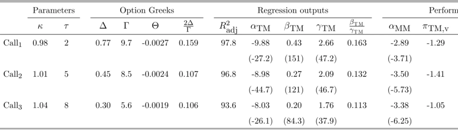
For each case, we …x the moneyness, time-to-maturity and portfolio weight of the option as constants. Every week, we recompute the delta, gamma and theta of the newly created option, and get an average over the whole sample period. With the time series of portfolio returns, we build the TM regression with total returns and estimate the TM, TM and TM coe¢ cients. From

these values, we compute the four performance measures designed around the TM model: TM,v

(Grinblatt and Titman, 1994); TM,a (Bollen and Busse, 2004); TM,o (Ingersoll et al., 2007) and

TM as proposed in equation (15). To improve precision, we adopt the weekly return on the risk-free

asset as the risk-free rate. Table 2 reports the results of this illustrative application. Insert Table 2 here

The options selection displays three levels of maturity and moneyness. The weight invested in options is set at w = 60%. The choice of portfolios for the illustration must be such that the ratio

2 _{, which is known ex ante from the choice of option characteristics, remains very close to the}

ex post ratio T M

T M retrieved from the quadratic regression of portfolio total returns on the market

index. Otherwise, the Taylor series expansion presented in equation (10) behaves too remotely from the regression (9). Under the market conditions that were prevailing during the sample period, it appears that only options with a strong convexity displayed this property6. The di¤erence between the two ratios is limited, as is oscillates from 2 to 19% relative to each other.

The linear alpha for each portfolio obtained with the market model is also reported. As expected from passive portfolios with a positive convexity, the alpha is negative and signi…cant in all three cases. The alpha from the quadratic regression is deeply negative, and requires a strong correction in order to avoid the threat of an easy manipulation. The additive corrections brought by the traditional approaches are too limited. The adjustment brought by taking the time value of the option into account in the expression for _TM are of an adequate order of magnitude. It leaves a performance value reasonably close too zero. Although these examples are illustrative and are not meant to provide statistical evidence, they emphasize at least that there are circumstances,

Keeping these returns makes the link between the quadratic beta and the option convexity too loose for a proper treatment, whatever the option maturity and moneyness considered.

when the quadratic mode speci…cation is good, where the association of option strategies to convex portfolio returns à la Treynor-Mazuy brings useful insight regarding their true return generating process.

3.2 The choice of the right option

We discuss the theoretical features of the best replicating option, then assess the empirical limi-tations a¤ecting this choice. The discussion focuses on a portfolio that achieves positive market timing, bearing in mind that a similar reasoning would hold for the mirror case of a negative market timer, which involves the sale of a put.

3.2.1 Option choice without constraints

Implementing a strategy that consists of replicating a portfolio with a long call option involves a careful selection of this option. As the underlying asset is determined by the selection of the index in the TM model, the choice collapses to setting the moneyness and the time-to-maturity of the option. The contract must respect a constraint, namely the target level of the ratio of the delta over its gamma in equation (14). Then, amongst all eligible options, the best is the one that minimizes the cost of replication, i.e. that maximizes expression w ; ; + (1 w ; ) Rf. The function to

maximize depends on the pair ( ; ) through the option theta, but also through the weight invested in the option in the passive portfolio w ; T M_; .

The partial derivatives of delta and gamma with respect to time are usually called Charm and Color, respectively (Garman, 1992). In the Black-Scholes-Merton world, they bear an analytical form and their behavior is well-known. Unfortunately, even in such a controlled environment, their sign is erratic. Haug (2003) shows an example where the Charm is negative for ITM and positive for OTM calls, but at the same time the Color is negative for near ATM and positive for far OTM or ITM options. Overall, the evolution of the ratio of delta over alpha over time (and so their derivative with respect to time-to-maturity) is indeterminate.

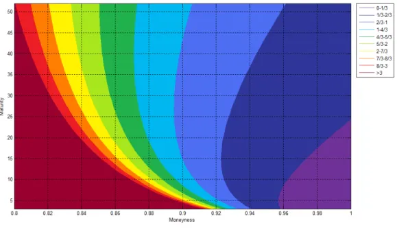
We illustrate in Figure 1 the sets of parameters that reach di¤erent target values of the ratio

T M

T M =

2 ;

; for options that are priced under the Black-Scholes-Merton model. We take as inputs

the average 3-month T-Bill rate and conditional volatility of the S&P500 weekly returns over the Jan. 1999 –Sept. 2008 period, namely 0.066% and 2.289%, respectively. The plotted contour lines correspond to target values of this ratio taking multiples of 1/3, ranging from 0 to 3. The ratio represents the fraction of beta over gamma in the TM model. As the average market beta is equal to one, we span in principle values of gamma starting from 1/3 on. We set the range of maturities to 1 to 52 weeks, and the range of moneyness ratios from 0.80 to 1.00.

Insert Figure 1 here Interpreting the ratio 2 ;

; as a reverse indicator of curvature, Figure 1 shows that only ITM

options (i.e. whose strike < 1) provide potentially meaningful convexity. For long maturity options, the progression of the ratio remains gradual. With a one-year maturity option, it takes a moneyness of ca. 90% to get a beta equal to half the option gamma or, by identity, a TM beta equal to its gamma. On the other hand, the ratio evolves very quickly with short maturity options. When the maturity approaches one week, i.e. the lowest maturity not lower than the frequency of returns estimation, the value of the ratio literally explodes when the moneyness gets lower than 93%.

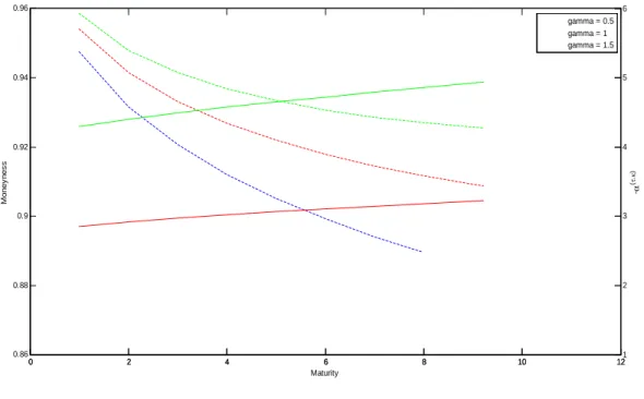
The next step of the analysis is to …nd out the cheapest-to-replicate option among the ones that respect a target ratio value. Following the same example as above, we set _TM = 1 and let the value of T M

T M equal to 2 (blue line), 1 (red line) and 0.67 (green line). They correspond, respectively, to the

contour lines between the dark and light green regions (ratio = 2), sky and light blue regions (ratio = 1) and light and dark blue regions (ratio = 0.67) in …gure 1. The _TM equals 0.5, 1.0 and 1.5, which are reasonable values for a market timer as shown later in our empirical study. For each feasible pair ( ; ), we compute the cost of the option replicating portfolio ( ; )= w ; ; (1 w ; ) Rf.

The lower this cost, the cheaper it is to replicate the option. Insert Figure 2 here

The replication cost increases with the level of _TM. This is the natural consequence of increasing the convexity of the portfolio payo¤, which is done at the expense of the option theta. The com-parison of the three lines shows quite small di¤erences between the patterns of the cost function. For _TM = 0:5 (blue line), the cost increases from 1.420% to 1.613%. The start and end points are 2.853% and 3.319% for _TM = 1; and 4.293% and 5.105% for _TM = 1:5; respectively. Thus, the cost increases slightly less than proportionally with the value of gamma and with maturity.7

In all illustrated cases, the option replication cost is an increasing function of option maturity. Even though this result cannot be generalized (because option Charm and Color have inde…nite signs), our realistic example shows that it can happen. It means that, in absence of any constraint on speci…c or approximation risk control, the cheapest-to-replicate option might have a maturity of one period. As it matches the frequency of returns computation, the option-based portfolio produces the returns of the HM model, and is unlikely to be adequately estimated using the TM speci…cation in the reverse regression. Hence, our case illustrates the need to assign constraints (21) and (22) for the reverse regression of option returns.

3.2.2 Option choice with approximation constraints

As indicated above, the option choice without constraints might realistically indicate that the shorter to maturity, the cheaper the option replication. The reverse quadratic regression (23) restricts the feasibility of maturity reduction because the quality of the …t naturally deteriorates as the option maturity decreases. The goal of this subsection is to detect, within the same setup as in the former example, the range of option maturities for which the approximation error induced by the Taylor series expansion is "acceptable", i.e. falls within the tolerance bounds for the alpha, beta and gamma retrieved from the quadratic regression.

We set portfolio beta equal to one and adopt the same set of TM gammas as before, namely 0.5, 1.0 and 1.5. The sample period is Jan. 1999 –Sept. 2008 and we create portfolios with a quadratic exposure on the S&P500 index. In order to ensure the correspondence between the Black-Scholes option prices and the behavior of the time series of index returns, we posit a ‡at weekly volatility of 2.375%. By using the sample standard deviation of returns in option prices, we avoid introducing a pricing bias in the estimation of regression (23). For each feasible pair ( ; ), a portfolio is constituted every week by investing a weight w ; in the option at a price C(M; ; ) and (1 w ; )

in the risk-free asset. The following week, the option is sold at a price C(M; 1;_(1+R

m)), the

risk-free return is booked on the remaining part, and the portfolio is rebalanced. We estimate the reverse quadratic regression by applying the TM speci…cation to the returns of this portfolio.

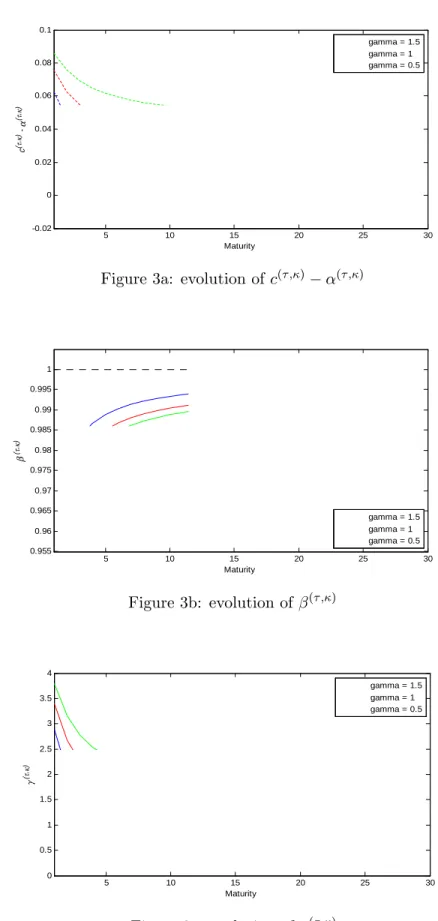
Figure 3 reports the evolution of the di¤erence between the intercept of the reverse regression and the analytical portfolio alpha, i.e. c( ; ) ( ; )(Figure 3a), the reverse regression beta (Figure 3b), and the reverse regression gamma (Figure 3c), as a function of the option time-to-maturity from 1 to 30 weeks. The values for _TM = 0:5, 1:0 and 1:5 are printed in green, red and blue, respectively.

Insert Figures 3a, 3b and 3c here

While the analytical replicating cost ( ; )increases with the option maturity, Figure 3a shows that the regression intercept c( ; )becomes closer to zero as time-to-expiration rises. Because of the poor regression …t for near-maturity options, c( ; ) _{starts at a very negative level (from 6:24%}

to 8:58%). As the regression signi…cance level increases with maturity, the intercept gradually approaches zero. In the cases illustrated by Figure 3, the two functions intersect at maturities equal to 23 weeks ( _TM = 0:5), 14.5 weeks ( _TM = 1:0) and 10.5 weeks ( _TM = 1:5). Figures 3b and 3c indicate that the convergence of the coe¢ cients for the linear and quadratic term asymptotically converge to their theoretical values. The speed of convergence typically decreases after a 5-week maturity. The linear coe¢ cient ( ( ; )) remains very close to its target value of 1, with a distance

becoming lower than 0.01 when the maturity exceeds 20 weeks. As expected from the imperfect …t of the second order approximation of the option return, the value of ( ; ) remains more remote. The coe¢ cient estimate remains systematically upward biased with respect to its target value. The explanation has to be found in the small variability of the observed squared market returns ( (R2

m) = 0:90% on a yearly basis) as compared to the returns themselves ( (Rm) = 17:13%). In

this OLS setup, the smaller variation in the independent variable translates into a larger standard deviation in the estimated coe¢ cient.

To get a more rigorous analysis of the set of option maturities that support reasonable coe¢ cient values for the reverse quadratic regression, we apply equations (21) and (22) to our data set. To re‡ect the volatility levels of the independent variables, the tolerance levels are adjusted by setting tol = =^tRm and tol = =^tR2

m for di¤erent values of a constant . This yields naturally

tol = j_^tRmj Rm + R2 m ^ t_R2 m

by applying equation (24). We set to 0.006, 0.004 and 0.002. These values are chosen so as to produce usable maturity intervals and to analyze how they shrink as the tolerance level decreases. The results are displayed in Table 3.

Insert Table 3 here

For each value of ; and , the table reports the maturity intervals that respect the tolerance

level for each parameter. The last row displays the intersection between these intervals. Interestingly, the intervals become thinner as the convexity of returns diminishes. The regression intercept yields the most severe constraint on the upper bound of the interval because, as shown in Figure 3a, the reverse regression intercept tends to become too large for longer maturities, while its theoretical value is supposed to decrease. For = 0:006, a large set of option maturities are acceptable, while the interval becomes an empty set for too low convexity and tolerance levels ( ; = 0:5 and = 0:002).

Overall, maturities between 18.9 and 26.8 weeks comply with most intervals: any maturity …ts for

; = 1:5, all from 24.8 to 26.8 weeks for ; = 1:0, and from 18.9 to 23.8 weeks for ; = 0:5.

The goal of this subsection is to identify the most satisfactory trade-o¤ between the regression …t and the accuracy of the intercept. The simulations indicate that, for reasonable values of the option convexity gamma of the replicating option, maturities around six months induce the best match between the regression results and the Taylor series expansion results of the option replicating strategy.

4

Empirical evidence on market timing revisited

We carry out an empirical analysis with a focus on funds that seem to exhibit a market timing behavior. Our major objective is to determine whether the performance attributable to these funds

would be substantially altered by the correction for the option replication cost. To achieve this goal, we perform two analyses. We …rst apply the Treynor and Mazuy model on a set of market timing funds and examine how various ways to correct the alpha for the timing ability of the manager a¤ect their performance assessment. In a second stage, we study the determinants of the adjusted performance, and attempt to detect whether there exists a genuine "market timing skill" that can be pointed out for di¤erent types of funds.

The analysis is performed on a sample of 2,521 U.S. equity mutual funds denominated in U.S. dollars with weekly returns spanning the period January 1999 –September 2008 (508 observations). The choice of weekly data represents a compromise between the superior ability to detect market timing e¤ects with higher frequency data (Bollen and Busse, 2001) and the evidence of higher potential bias due to benchmark misspeci…cation with the use of daily fund returns (Coles et al., 2006). The comparability of the parameter estimates is warranted by retaining the 1,242 funds with a full return history over the period.8 The fund characteristics and returns are retrieved from Bloomberg. Index funds and multiple share classes are excluded from the analysis. To ensure consistency across the various model speci…cations, all index returns as well as the risk-free rate are extracted from Kenneth French’s online data library.

4.1 Reestimating the Treynor-Mazuy performance

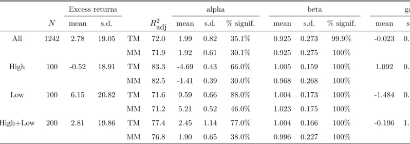
The Treynor and Mazuy speci…cation in excess returns, corresponding to equation (9), is estimated on each individual fund during the period using the White heteroskedasticity-consistent estimation method. We further select the "best" market timers by identifying the 100 funds displaying the highest t-stat for the estimated quadratic coe¢ cient ( _TM).9 We call it the "High" subsample. Likewise, the 100 "worst" market timers are those displaying the 100 most negative values of the student statistic for the same coe¢ cient _TM. We call this subsample the "Low" one. The descriptive statistics for the global sample and the three subsamples are reported in Table 4.

Insert Table 4 here

The adoption of the Treynor and Mazuy speci…cation does not bring a sensitive improvement over the market model (MM) overall. Only when the market timing is pronounced, the adjusted R-squared increases by 0.5% on average, while the estimated alpha of market timers naturally decreases in absolute value by accounting for the funds’convexity.

8

As the objective is not to perform a comprehensive assessment of mutual fund performance, the resulting survivorship bias does not a¤ect the output of the study.

9

The TM statistics for the individual sub-samples High and Low substantially di¤er from the overall sample on all criteria except for the market beta, which is remarkably similar across samples. Positive market timers record slightly negative excess returns, negative alphas and strong positive gammas. The exact opposite holds for the Low set. Overall, the estimates are more favorable for the Low subsample regarding both excess and abnormal returns, but the negative convexity of the TM regression is more pronounced as well. The average excess return, alpha and beta from the whole sample are close to the ones of the combined High+Low sub-samples featuring the 100 best and 100 worst market timers. Because the absolute values of alpha and gamma of market timing funds are often greater and more signi…cant than for the rest of the sample, the High+Low sub-sample exhibits highly dispersed values for these parameters.

Henceforth, we focus on the High, Low, and High+Low subsamples. For each fund, the repli-cating option is priced under the Black-Scholes-Merton formula. As we deal with retrospective performance evaluation, we use the in-sample stock market volatility and average interest rate. They are set to a yearly 17.16% and 3.495%, respectively. Consistently with our discussion in the previous section, a constant option maturity of 0.5 year (26 weeks) is taken for all options. The option moneyness i for each fund i then equates

2 _{0:5; i}

0:5; i = T M ;i

T M ;i. In case the estimated coe¢ cient

TM;i is positive, the alpha is adjusted through the cost of replicating a call option as in equation

(15). If gamma is negative, the replicating portfolio involves a put option, and the alpha is corrected according to equation (17).

From the original estimate of TM;i, two types of adjustments are tested: the variance

cor-rection _TM;i 2

m (Grinblatt and Titman, 1994), and the cost of the replicating option equal to

w0:5; i TM;i Rf w0:5; i 0:5; i for a call ( TM;i> 0) or w0:5; i+ TM;i Rf+ w0:5; i 0:5; i

for a put ( _TM;i< 0).10 The statistics of the corrections and of the resulting performance metrics

TM,v and _TM are reported in Table 5. For comparison purposes, we also reproduce the

statis-tics for the alphas generated by applying the market model ( MM) as well as those obtained by

applying the Fama and French (1993) - Carhart (1997) four-factor model with the size, value and momentum portfolios ( 4F).11 The table also provides information on the frequency of signi…cantly

positive or negative estimates of performance. For the adjusted values TM,v and TM, we compute

bootstrapped standard errors.

Insert Table 5 here

1 0

The corrections proposed by Bollen and Busse (2004) and Ingersoll et al. (2007) produce very similar results to the variance correction approach, and are not reported to save space. Detailed results are available upon request.

1 1_{We do not present results with one or several market timing coe¢ cients to the four-factor model as this}

The variance correction approach performs only a limited average adjustment over the initial TM alpha. As a result, the adjusted alpha of market timers tends to re‡ect a sign opposite to their gamma: a low performance for positive market timers, and a high one for negative market timers. This phenomenon would lead to the conclusion that a large number (almost one third) of the fund managers belonging to the High sample underperform the market. The diagnosis would be more extreme for negative market timers: out of the 100 managers, almost one half (45%) would be supposed to beat the market. The corrected alphas are very close to the initial alphas measured with the market model.

By contrast, the application of the portfolio replication adjustment leads to a large correction, which even results in switching the sign of alpha for the Low subsample. On average, the application of this technique delivers a negative performance for both the positive and negative market timers, even though the average performance is very close to zero in the High subsample. 3.5% of the positive market timers deliver signi…cant positive alphas, and only 10.5% display underperformance. These …gures are closest to the ones obtained with the four-factor (4F) model, even though the portfolio replication approach would be more generous in the High sample (7 outperformers against only 3 for the 4F model). Note anyway that the proportion of outperformers is lower than the critical rejection level (10%). Thus, these superior funds could be due to luck, and a proper control for "false discoveries" as proposed by Barras et al. (2010) could lead all performance to fade away. With negative market timers, the four-factor model concludes more often to abnormal (positive or negative) performance. None of them beats the market when the _TM measure is used instead.

The explanation of such a large observed di¤erence between the correction techniques could come from two possible sources. The …rst one would be the relative inability of the variance of market returns to re‡ect the cost (or bene…t) of replicating a deep OTM option. By applying a linear penalty or reward for the manager’s convexity parameter _TM, the traditional variance correction technique underestimates the correction to be applied. Oppositely, the theta of the replicating option more properly accounts for the price of convexity. The phenomenon is particularly noticeable for the Low sample, characterized by very negative values of the quadratic term in the TM regression. The second explanation for the observed di¤erences in performance corrections would be a systematic bias in the application of the option replication technique, for instance by taking a too cheap option, thereby exaggerating the adjustment for both positive and negative market timers. This conjecture is investigated in the next section.

Economically, the variance correction approach yields an average abnormal performance of 5.22% per annum, which is highly unlikely to truly re‡ect the actual skills of this group of managers. The picture delivered by the option portfolio replication method is much more consistent with the evidence of spurious market timing emphasized by Warther (1995) and Edelen (1999), according to

whom negative market timing coe¢ cients mostly result from a fund ‡ows explanation.

Besides its magnitude, the variability of the correction induced by the portfolio replication approach exceeds the one of the variance correction as well. The reason underlying this higher volatility has to be found in the explicit account for the fund’s beta (and therefore its cross-sectional dispersion in each sample) in the portfolio replication technique.

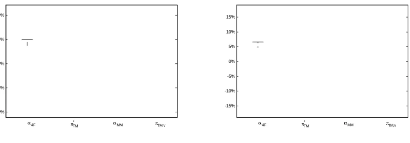
Table 5 also suggests that alphas corrected with the portfolio replication approach are typically slightly negative, even more than the four-factor alphas. Figure 4 provides a synthetic representation of the distribution of performance measure estimates for the High and Low subsamples through a box-and-whisker graph.

Insert Figure 4 here

In both graphs, the distributions of TM,v and MM appear identical, while the main

charac-teristics of the empirical distributions of 4F and TM are quite similar. We focus on this second

…nding. Figure 4a (High subsample) shows a similar median, but greater dispersion and, in partic-ular, right skewness of the distribution of _TM. In Figure 4b (Low subsample), the distribution of

TM is shifted down with respect to the one of 4F. Together with the diverging evidence evidence

on signi…cance levels reported in Table 4, these …ndings suggest that the four-factor model and the Treynor-Mazuy model with the portfolio replication adjustment produce relatively close ranges of alphas, but they are distributed quite di¤erently across funds. This calls for further analysis of the comovements between each fund’s various performance metrics, and possibly the identi…cation of common patterns that would explain the fund managers’ performance levels. This is done is the next subsection.

4.2 Revisiting the market timing skills

After having justi…ed the relevance of the portfolio replication approach to adjust the performance of a market timer, it is relevant to consider the drivers of this performance. We …rst examine whether a clear pattern of performance generation can be extracted from the data. This is done through a correlation analysis, as shown in Table 6.

Insert Table 6 here

In both samples, the correlation between TM,v and TM is very high, as expected. However

their relationship with the original TM performance metrics TM and TM is very di¤erent.

When the variance correction is applied, the convexity e¤ect induced by _TM either vanishes (High subsample) or negatively correlates with abnormal performance (Low subsample). Thus, for

positive market timers, the value of TM,v is almost entirely driven by the TM alpha. Because in the

second case _TM is always negative, the negative correlation implies that a higher market timing e¤ect goes along with higher performance. This can be interpreted as a natural consequence of the inability of the variance adjustment to translate very high values of gamma into an adequate penalty.

The correlation structure of performance measures in the High and Low samples vary to a large extent. The properties of _TM for negative market timers are similar, although slightly less pronounced, to the ones of TM,v: a very high in‡uence of TM, a moderate but signi…cant impact

of _TM. On the other hand, the correlation between the variance-corrected performance TM,v and

the initial alpha estimated with the market model MM is almost perfect. This …nding suggests that

negative market timers do not "time" the market at all; they merely get exposure to the market portfolio and behave as if they sell call options to enhance their returns through the time value of the option premium. What Table 6 shows is that the traditional ways to adjust the TM alpha when the gamma is negative are powerless: they simply lead back to the original linear alpha, which is largely positive. They provide a false impression of abnormal performance. In this context, the main value-added of the portfolio replication approach lies in the magnitude of the correction, not in its discrimination between market timing vs. asset selection skills. On average, performance vanishes when a proper correction is applied, as the Low sample mean of -1.83% shown in Table 5 indicates. In the High subsample however, the covariation between _TM and TM becomes moderate, while

the e¤ect of _TM on _TM is stronger, at least in values (the rank correlations are almost identical). The performance metrics obtained with linear asset pricing models, MM and 4F, hardly covary

with the portfolio replication-adjusted performance _TM. This …nding can be related to the graphical evidence of Figure 4: even though the means of 4F and TM are close, their marginal distributions

are remote from each other.

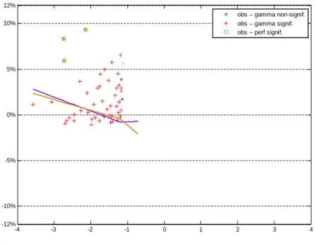
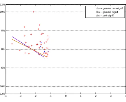
We speci…cally examine the relation between each fund’s risk- and market timing-adjusted per-formance and its indicator of market timing. The rationale for this investigation is a straightforward consequence of the adjustment in the market timing context. If fund managers attempt to time the market, one can expect that the ones who record a signi…cant abnormal performance indeed suc-cessfully timed the market. In other terms, the market timing skill hypothesis suggests that the adjusted alpha is an increasing function of the absolute value of gamma. Oppositely, when gamma is close to zero, the performance of fund managers should not show any signi…cant relationship with the fund’s convexity. Because funds that display no market timing behavior should not be rewarded for their pretended market timing skills, any evidence of a relationship between gamma and a performance measure would indicate an imperfect adjustment for market timing, resulting in a biased estimate of performance.