593
Q2004 Estuarine Research Federation
Variability of the Gas Transfer Velocity of CO
2in a Macrotidal
Estuary (the Scheldt)
ALBERTO VIEIRABORGES1,*, JEAN-PIERREVANDERBORGHT2, LAURE-SOPHIESCHIETTECATTE1,
FRE´ DE´RICGAZEAU1, 3, SARAHFERRO´ N-SMITH4, BRUNO DELILLE1, and MICHEL
FRANKIGNOULLE1
1Universite´ de Lie`ge, MARE, Unite´ d’Oce´anographie Chimique, Institut de Physique (B5), B-4000 Sart-Tilman, Belgique
2Universite´ Libre de Bruxelles, Laboratoire d’Oce´anographie Chimique et Ge´ochimie des Eaux, CP 208, Campus de la Plaine, B-1050 Bruxelles, Belgique
3Laboratoire d’Oce´anographie de Villefranche, UMR 7093 CNRS-UPMC, B. P. 28, F-06234 Villefranche-sur-mer Cedex, France
4Universidad de Ca´diz, Facultad de Ciencias del Mar y Ambientales, Campus Rı´o San Pedro S/n 11510 Puerto Real, Espan˜a
ABSTRACT: We report a large set of 295 interfacial carbon dioxide (CO2) flux measurements obtained in the Scheldt estuary in November 2002 and April 2003, using the floating chamber method. From concomitant measurements of the air-water CO2 gradient, we computed the gas transfer velocity of CO2. The gas transfer velocity is well correlated to wind speed and a simple linear regression function gives the most consistent fit to the data. Based on water current measurements, we estimated the contribution of water current induced turbulence to the gas transfer velocity, using the conceptual relationship of O’Connor and Dobbins (1958). This allowed us to construct an empirical relationship to compute the gas transfer velocity of CO2that accounts for the contribution of wind and water current. Based on this relationship, the spatial and temporal variability of the gas transfer velocity in the Scheldt estuary was investigated. Water currents contribute significantly to the gas transfer velocity, but the spatial and temporal variability (from daily to seasonal scales) is mainly related to wind speed variability.
Introduction
A rigorous estimation of the exchange of carbon dioxide (CO2) across the air-water interface is
crit-ical to determine ecosystem metabolism (Smith and Key 1975) and to budget the annual sink or source for atmospheric CO2 at local (Borges and
Frankignoulle 2002), regional (Lefevre et al. 1999), and global scales (Takahashi et al. 2002). The flux of CO2across the air-water interface (F)
can be computed according to:
F 5 kaDpCO2 (1)
wherea is the solubility coefficient of CO2,DpCO2
is the air-water gradient of the partial pressure of CO2 (pCO2), and k is the gas transfer velocity of
CO2(also referred to as piston velocity). A positive
F indicates a transfer of CO2from the water to the
atmosphere.
Because highly precise and accurate methods to measure DpCO2are now available, the largest
un-certainty in the computation of F comes from the k term in both open oceanic and coastal
environ-* Corresponding author: tele:13243663187; fax: 1323662355; e-mail: [email protected]
ments. Based on numerous theoretical, laboratory, and field studies, it is well established that the most important process controlling k is turbulence at the air-water interface (in the case of sparingly sol-uble gases such as CO2 the critical process is
tur-bulence in the liquid phase). In open oceanic wa-ters, the gas transfer velocity of CO2 is usually
pa-rameterized as a function of wind speed, because wind stress is the main generator of turbulence in these systems. At low wind speeds, the air-water gas transfer is further modulated by the presence of surfactants, convective cooling, chemical enhance-ment, and rain. At high wind speeds, capillary and gravity waves, bubbles, and spray also strongly con-tribute to air-water gas transfer.
Gas transfer velocities in estuaries have been es-timated from the mass balance of naturally occur-ring or opportunistic tracers such as Chlorofluo-rocarbons (Clark et al. 1992) and 222Rn (Elsinger
and Moore 1983; Hartman and Hammond 1984, 1985), from the mass balance of purposeful trac-ers,3He and SF
6(Clark et al. 1994, 1996; Carini et
al. 1996), from the mass balance of O2 (Devol et
al. 1987), and from floating chamber measure-ments of222Rn (Hartman and Hammond 1984;
De-vol et al. 1987; Richey et al. 2002), O2(Marino and
Howarth 1993; Richey et al. 2002; Kremer et al. 2003a), and CO2(Borges et al. 2004). The floating
chamber technique provides gas transfer velocity estimates at short time scales (minute), compared to the tracer mass balance approaches (hour to day), but it has been dismissed by several workers (e.g., Liss and Merlivat 1986; Raymond and Cole 2001). One of the critiques is that the chamber covers the water surface and eliminates wind stress. For sparingly soluble gases such as CO2, gas
trans-fer is controlled by turbulence in the liquid phase. If the floating chamber does not disrupt the un-derlying water turbulence, then the corresponding gas transfer measurements should be reasonable estimates of those from the undisturbed surface. The disturbance of the floating chamber on the surface wind boundary layer was tested experimen-tally by Kremer et al. (2003b). They measured O2
fluxes using a floating chamber with an adjustable speed fan to generate air turbulence and a control floating chamber. Under moderate wind condi-tions, the additional air turbulence from the fan only increased the fluxes by 2–12% compared to the control chamber. Kremer et al. (2003b) also report a series of experiments comparing the float-ing chamber technique with mass balance ap-proaches of O2, 222Rn, and 3He in various
experi-mental settings (laboratory tanks, outdoor tanks, mesocosms, and lakes). Fluxes based on the float-ing chamber technique agreed with the other di-rect methods within 10–30%. Two publications re-port large discrepancies between the floating chamber technique and other approaches (Belan-ger and Korzum 1991; Matthews et al. 2003) that, in our opinion, highlight the limits of the method rather than dismiss it altogether. Belanger and Kor-zum (1991) compared O2evasion rates from pools
by a mass balance approach and floating chamber measurements. They concluded that the floating chamber measurements were biased by tempera-ture and pressure changes during the experiments. The duration of these measurements was several hours, and temperature and pressure changes are not expected to interfere during very short de-ployments of the floating chamber (such as in our case). Matthews et al. (2003) compared k estimates in a small sheltered boreal reservoir, based on floating chamber and SF6evasion techniques.
Dur-ing their experiment, wind speeds were extremely low, on average 0.2 m s21and never exceeding 0.5
m s21. As noted by Kremer et al. (2003b), the
flux-es measured in nearly motionlflux-ess waters with a floating chamber should be taken with caution. Also, estuarine environments (such as in our case) are expected to be much more turbulent due to
tidal currents than the reservoir studied by Mat-thews et al. (2003).
Another critique of the floating chamber tech-nique is that the interference from the chamber itself would result in artificially high k estimates. This issue will remain unresolved until a field in-tercomparison of methods is carried out; the next best approach is the comparison of k-wind rela-tionships in similar systems. Figure 1 shows that k estimates from floating chamber CO2
measure-ments in two coral reef systems reported by Fran-kignoulle et al. (1996a) follow the McGillis et al. (2001) relationship for wind speed below 6 m s21.
At wind speeds above 6 m s21, the k estimates given
by Frankignoulle et al. (1996a) are in fact below the values computed from the Liss and Merlivat (1986) parameterization. The generic relationship of Marino and Howarth (1993) that includes k es-timates from floating dome O2 measurements in
lakes, estuaries, and open oceanic waters falls be-tween the parameterizations from Jacobs et al. (1999) and McGillis et al. (2001). In estuaries, the relationship of Kremer et al. (2003a) based on floating chamber O2 measurements in Sage Lot
Pond and Childs River estuaries is well below the parameterization from Clark et al. (1995) based on tracer measurements in the Hudson River and San Francisco Bay (Fig. 1). The relationship from Ma-rino and Howarth (1993) refitted taking into ac-count exclusively the floating chamber O2
mea-surements in the Hudson River are above the Clark et al. (1995) parameterization. As noted by Ray-mond and Cole (2001) gas tracer experiments measure average gas transfer velocities over long time scales (days to weeks) compared to floating dome measurements that give virtually immediate estimates. The higher k values reported by Marino and Howarth (1993) compared to those by Clark et al. (1995) could be due to short-term enhance-ment related to the contribution of water currents to interfacial turbulence. Peak-flow water currents of 40 and 200 cm s21were reported by Clark et al.
(1995) and Marino and Howarth (1993), respec-tively. Zappa et al. (2003) report k values based on the vertical gradient technique in Plum Sound es-tuary that are up to 8 cm h21 higher at the same
wind speed than the estimates from Carini et al. (1996) based on SF6 release experiment in the
same estuarine system. This value corresponds roughly to the difference between the estimates based on the Marino and Howarth (1993) and the Clark et al. (1995) parameterizations at a wind speed of 6 m s21.
Based on a large data set of floating chamber CO2 flux measurements in three European
estu-aries (Randers Fjord, Scheldt and Thames), we re-cently showed that a simple parameterization of k
FIG. 1. Comparison of gas transfer velocity parameteriza-tions as a function of wind speed in open oceanic waters and estuaries. The Liss and Merlivat (1986) relationship is based on a SF6release experiment in a lake by Wanninkhof et al. (1985) and wind tunnel experiments by Broecker and Siems (1984) (L&M86; solid bold line). The Jacobs et al. (1999) relationship is based on gradient flux technique measurements (wind speed range 3–14 m s21) in the North Sea ( J99; bold short dashed line). The Nightingale et al. (2000) relationship is based on two SF6and3He release experiments (wind speed range 3–14 m s21) in the North Sea (N00; long dashed line). The McGillis et al. (2001) relationship is based on direct covariance technique measurements (wind speed range 1–16 m s21) in the North At-lantic Ocean (McG01; solid line). The Marino and Howarth (1993) relationship is based on floating dome O2measurements (wind speed range 0–10 m s21) in various estuaries, lakes, and open oceanic waters (M&H93; dashed-dotted line). The F96 re-lationship is based on the original data from Frankignoulle et al. (1996a) of floating dome CO2measurements (wind speed range 0–11 m s21) in Yonge Reef and Moorea coral reefs. The k660 data were averaged over wind speed bins of 1 m s21 (squares). The best fit to the data is given by k6605 3.6(60.7) 1 0.07(60.07)u10(2.260.4)(r25 0.952, n 5 11) (F96; short dashed line). The Kremer et al. (2003a) relationship is based on float-ing dome O2measurements (wind speed range 0–8.5 m s21) in Childs River and Sage Lot Pond estuaries (K03; dashed line). The Clark et al. (1995) relationship is based on SF6release ex-periments (wind speed range 1–6.5 m s21) in the Hudson River estuary and222Rn mass balance in San Francisco Bay (C95; solid line). The Carini et al. (1996) is based on a SF6release experiment
←
(wind speed range 0–2 m s21) in Park River estuary (C96; bold solid line). The Zappa et al. (2003) data are based on gradient flux technique measurements in Plum Island Sound (Parker River) estuary during a half tidal cycle at constant low wind speed (1.9 m s21) (Z03; open circles). The H&M93 relationship is based on the original data from Marino and Howarth (1993) of floating dome O2measurements (wind speed range 0–6.5 m s21) in the Hudson River estuary. The best fit to the unbinned data is given by k600 5 1.1(64.0) 1 1.7(62.2)u10(1.460.7)(r25 0.864, n5 9) (H&M93 refit; dashed-dotted line). Note different x and y scales in plots A and B; k is normalized to a Schmidt number of 660 and 600 in plots A and B, respectively.
as a function of wind speed is estuary specific (Bor-ges et al. 2004). This is related to the fact that the contribution to the gas transfer velocity of CO2
from turbulence generated by tidal currents is neg-ligible in microtidal estuaries such as the Randers Fjord, but is substantial in macrotidal estuaries such as the Scheldt and Thames. The aim of the present work is to study the temporal and spatial variability of k in the Scheldt estuary based on a recently obtained data set of interfacial CO2 flux
measurements using the floating chamber tech-nique.
Materials and Methods
During two cruises in the Scheldt estuary (No-vember 2002 and April 2003), 9 stations were oc-cupied for 24 h and flux measurements were car-ried out approximately every 10 min during day-time (Table 1).
pCO2 was measured (1-min recording interval)
with a nondispersive Infra-Red Gas Analyser (IRGA) in air equilibrated with subsurface water (pumped from a depth of 2.5 m). For a detailed description of the equilibration technique and cal-ibration procedures of the IRGA refer to Frankig-noulle et al. (2001) and FrankigFrankig-noulle and Borges (2001).
The air-water CO2fluxes were measured with the
floating chamber method from a drifting rubber boat in order to avoid the interference of water turbulence within the chamber created by the pass-ing water current observed in earlier measure-ments carried out from a fixed point (Frankig-noulle unpublished data). Care was taken to main-tain the floating chamber about 2 to 3 m away from the rubber boat to avoid interference on the air and water boundary layers. The chamber is a plastic right circular cone (top radius 5 49 cm; bottom radius5 57 cm; height 5 28 cm) mounted on a float, and connected to a closed air loop with an air pump (3 l min21) and an IRGA, both
pow-ered with a 12 V battery. The IRGA was calibrated daily using pure nitrogen and a gas mixture with a CO2molar fraction of 351 ppm. The readings of
T ABLE 1. A verage (6 standard deviation) of depth, wind speed (u 10 ), water cur rent (w), salinity , pCO 2 in subsur face water (pCO 2water ), atmospheric pCO 2 (pCO 2air ), atmospheric CO 2 flux (F), and the gas transfer velocity of CO 2 (k 600 ) a t 9 stations in the Scheldt estuar y, sampled in November 2002 and April 2003 (n indicates the number of measurements). Date Longitude (8 E) Latitude (8 N) Depth (m) u10 (m s 2 1) w (cm s 2 1) Salinity pCO 2water (ppm) pCO 2air (ppm) F (mmol m 2 2d 2 1) k600 (cm h 2 1)n November 6, 2002 November 8, 2002 November 10, 2002 November 12, 2002 April 2, 2003 April 4, 2003 April 6, 2003 April 8, 2003 April 9, 2003 4.314 4.399 4.040 4.215 4.303 4.250 4.399 3.931 4.164 51.127 51.226 51.410 51.395 51.124 51.348 51.226 51.381 51.381 13 11 14 17 12 14 9 15 19 4.0 (0.2) 6.8 (0.2) 7.5 (0.3) 8.4 (0.5) 8.2 (0.3) 3.3 (0.1) 5.1 (0.2) 4.7 (0.2) 7.1 (0.2) 86.1 (3.5) 18.8 (5.6) 48.4 (4.8) 9.6 (2.6) 82.2 (4.3) 43.1 (6.2) 73.0 (6.9) 61.5 (5.8) 27.2 (3.7) 0.41 (0.01) 0.49 (0.02) 13.31 (0.38) 7.69 (0.16) 0.57 (0.01) 6.29 (0.14) 1.22 (0.13) 19.29 (0.13) 9.38 (0.25) 7,358 (22) 6,959 (11) 1,403 (48) 2,229 (28) 6,451 (35) 2,917 (56) 5,756 (107) 789 (6) 1,840 (55) 381 (1) 393 (1) 396 (1) 387 (1) 374 (1) 386 (1) 373 (1) 381 (1) 379 (1) 980 (375) 1,377 (438) 259 (141) 516 (95) 1,244 (448) 251 (66) 925 (247) 65 (26) 311 (114) 15 (1) 22 (1) 27 (2) 30 (2) 21 (1) 11 (1) 18 (1) 19 (1) 23 (1) 28 32 38 14 38 40 36 42 27
FIG. 2. The gas transfer velocity of CO2(k600in cm h21) as a function of wind speed at 10 m height (u10in m s21) in the Scheldt estuary and two published relationships. The open squares correspond to k600from which the contribution of water currents was removed (k600wind). The contribution of water cur-rents to k600was estimated from the conceptual relationship of O’Connor and Dobbins (1958), using water current measure-ments concomitant to the CO2flux measurements and it was removed from individual k600estimates before the data were bin averaged. The data were averaged over wind speed bins of 1 m s21(error bars correspond to the standard deviations on the bin averages). The error bar on top left corner of the plot corre-spond to the average uncertainty on k600, estimated using the individual standard error on the slope of the regression of pCO2 in the floating chamber against time (from which the CO2flux was computed see the Materials and Methods) and assuming an error onDpCO2of63%. The Raymond and Cole (2001) rela-tionship (k6005 1.91 exp(0.35u10)) is based on a compilation of published k600values in various rivers and estuaries and ob-tained using different methods (floating chamber, natural trac-ers [CFC,222Rn], and purposeful tracer [SF
6]). The Clark et al. (1995) relationship (k600 5 2 1 0.24u102) is based on a dual tracer (3He and SF
6) release experiment in the Hudson River estuary and222Rn mass balance in San Francisco Bay from Hart-man and Hammond (1984). Note that the Clark et al. (1995) and the Raymond and Cole (2001) relationships are con-strained by data obtained at wind speeds below 6.5 m s21(bold in the plot). The Zappa et al. (2003) data are based on gradient flux technique measurements in Plum Island Sound (Parker River) estuary during a half tidal cycle at constant low wind speeds (1.9 m s21) (Z03; open circles). Solid lines correspond to the linear regression functions of k600observedand k600wind(Eqs. 2 and 13, respectively).
FIG. 3. Monthly averages for 1997–2001 of the gas transfer velocity of CO2(k600in cm h21) computed from Eq. 14 from hourly wind speed measurements (u10in m s21) and modelled water currents at three reference stations (Vlissingen, Han-sweert, and Antwerpen; see Table 3 for geographical positions), and the percentage of contribution of water currents to the gas transfer velocity of CO2(%w).
TABLE 2. Equations of fits of the gas transfer velocity of CO2(k600in cm h21) as a function of wind speed at 10 m height (u10in m s21), using various functions, in the Scheldt estuary (November 2002 and April 2003). ABS5 absolute sum of residuals squares. r2 and ABS of the three best fits discussed in text are in bold.
Equation Type Equation Formulation Eq. r2 ABS
y5 a 1 bx y5 a 1 bx2 y5 ax2 y5 a 1 bx3 y5 ax3 y5 a 1 bxc y5 axc y5 a 1 b.exp(cx) y5 a.exp(bx) k6005 4.045 1 2.580u10 k6005 10.07 1 0.201u102 k6005 0.3501u102 k6005 13.10 1 0.0179u103 k6005 0.0355u103 k6005 23.065 1 7.302u100.646 k6005 5.141u100.758 k6005 2897.5 1 901.6exp(0.0687u10) k6005 8.7exp(0.01503u10) 2 3 4 5 6 7 8 9 10 0.955 0.892 0.095 0.807 0.000 0.961 0.960 0.954 0.914 24.9 59.6 499.0 106.6 987.2 21.48 21.85 25.13 47.69
pCO2 in the chamber were written down every
30 s during 5 min. The flux was computed from the slope of the linear regression of pCO2against
time (r2usually$0.99) according to Frankignoulle
(1988). The uncertainty of the flux computation due to the standard error on the regression slope is on average 63%. The gas transfer velocity of CO2 was computed from the interfacial CO2 flux andDpCO2measurements (atmospheric pCO2was
measured and recorded at the start of each flux measurement), using the CO2solubility coefficient
formulated by Weiss (1974) and normalized to a Schmidt number (Sc) of 600 (k600), assuming a
de-pendency of the gas transfer velocity proportional to Sc20.5. The Schmidt number was computed for
a given salinity from the formulations for salinity 0 and 35 given by Wanninkhof (1992) and assuming that Schmidt number varies linearly with salinity.
During both cruises, wind speed was measured at 18 m height with a Friedrichs 4034.000 BG cup anemometer, and, recorded every 10 s. Winds speeds were referenced to a height of 10 m (u10)
according to Smith (1988), using concomitant air and water temperature measurements and were av-eraged for the period of each flux measurement. Water current speeds in subsurface waters mea-sured with an Aanderaa RCM7 were recorded ev-ery minute and were also averaged for the period of each flux measurement.
Temporal series of hourly u10 measurements
were provided by the Koninklijk Nederlands Me-teorologish Instituut at Vlissingen and Hansweert and by Belgocontrol at Antwerpen. At these three reference stations, hourly water currents were com-puted using a 1-dimensional hydrodynamic model of the Scheldt estuary (CONTRASTE, Regnier et al. 1997). The boundary conditions for the simu-lation are obtained from a tide prediction routine taking into account the spring-neap oscillation at the estuarine mouth and from the daily value of the freshwater discharge measured at the upper limit of the tidal rivers.
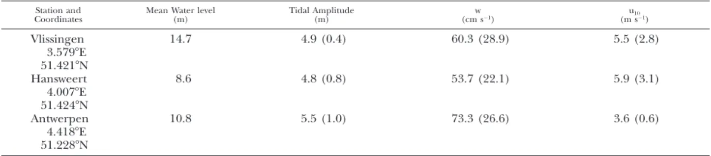
TABLE 3. Average (6 standard deviation) of time series (1997–2001) of tidal amplitude, water current (w), and wind speed (u10) at three reference stations in the Scheldt estuary.
Station and
Coordinates Mean Water level(m) Tidal Amplitude(m) (cm sw21) (m su1021)
Vlissingen 3.5798E 51.4218N 14.7 4.9 (0.4) 60.3 (28.9) 5.5 (2.8) Hansweert 4.0078E 51.4248N 8.6 4.8 (0.8) 53.7 (22.1) 5.9 (3.1) Antwerpen 4.4188E 51.2288N 10.8 5.5 (1.0) 73.3 (26.6) 3.6 (0.6)
TABLE 4. Average (6 standard deviation) of water current (w), wind speed (u10), gas transfer velocity of CO2(k600), percentage of contribution of water currents to the gas transfer velocity of CO2 (%w) and percentage of contribution of wind speed to the gas transfer velocity of CO2(%u10), computed according to Eq. 14, using hourly observed wind speed and modelled water current data series at three reference stations in the Scheldt estuary 1997–2001.
Year Vlissingen w (cm s21) (m su1021) (cm hk60021) (%)%w %u(%)10 Hansweert w (cm s21) (m su1021) (cm hk60021) 1997 1998 1999 2000 2001 Mean 60.8 (29.0) 60.8 (28.9) 60.3 (29.0) 59.6 (28.7) 59.6 (28.5) 60.2 (28.8) 5.2 (2.7) 5.7 (2.9) 5.5 (2.8) 5.7 (2.8) 5.3 (2.6) 5.5 (2.8) 17.7 (7.2) 19.1 (7.5) 18.5 (7.3) 19.0 (7.4) 18.1 (6.8) 18.5 (7.2) 21.9 (10.4) 20.2 (9.9) 20.8 (10.5) 20.3 (10.3) 21.1 (10.2) 20.8 (10.3) 78.1 (10.4) 79.8 (9.9) 79.2 (10.5) 79.7 (10.3) 78.9 (10.2) 79.2 (10.3) 54.0 (22.1) 54.0 (22.0) 53.6 (22.2) 53.0 (22.0) 53.1 (21.9) 53.6 (22.0) 5.4 (3.1) 6.2 (3.2) 5.9 (3.1) 6.2 (3.1) 5.9 (2.9) 5.9 (3.1) 19.0 (8.2) 20.8 (8.5) 20.3 (8.2) 20.7 (8.3) 20.3 (7.6) 20.2 (8.2)
Results and Discussion
DATASET OVERVIEW
A total of 295 CO2 flux measurements were
car-ried out for both cruises, at 9 stations in the Scheldt estuary (Table 1). A large fraction of the salinity gradient was covered during both cruises with values ranging from 0.4 to 21. Oversaturation of CO2of surface waters with respect to
atmospher-ic equilibrium was systematatmospher-ically observed during both cruises with pCO2values ranging from 716 to
7,553 ppm. The largest difference between the two cruises in the distribution of pCO2 versus salinity
(not shown) was observed in the upper estuary, with pCO2 values on average higher at salinity 0.4
during the November 2002 cruise (Table 1). At-mospheric pCO2 values ranged from 368 to 422
ppm, and values for both cruises were on average 9 ppm above the uncontaminated pCO2 signal
from Weather Station Mike (66.008N, 2.008E), rep-resentative of the open North Sea waters (from the National Oceanic and Atmospheric Administra-tion, Climate Monitoring and Diagnostics Labora-tory air samples network, available from the inter-net at http://www.cmdl.noaa.gov/). The interfa-cial CO2 fluxes were positive during both cruises,
ranging from 31 to 2,189 mmol m22 d21. Wind
speed values ranged from 1.6 to 11.0 m s21. About
61% of the interfacial CO2 flux measurements
were obtained at wind speeds ranging from 3.0 to
7.0 m s21. About 1.4% and 4.4% of the interfacial
CO2 flux measurements were obtained at wind
speeds below 2 m s21 and above 10 m s21,
respec-tively. Water currents ranged from 1 to 130 cm s21
and unlike wind speed, the CO2 flux
measure-ments were regularly distributed over the water current range of variation.
GAS TRANSFERVELOCITYPARAMETERIZATION AS A
FUNCTION OFWIND SPEED
Figure 2 shows the averaged k600over wind speed
bins of 1 m s21versus wind speed. A steady increase
of k600 with wind speed is observed, and for wind
speeds above 6 m s21, the k
600values fall within the
range of values from existing parameterizations of k600 in estuaries. For wind speeds below 6 m s21,
the k600 values are above any of the published
pa-rameterizations of k600as a function of wind speed.
At a wind speed of 2 m s21, k
600 values in the
Scheldt are within the range of values reported by Zappa et al. (2003) based on the gradient flux technique, during a half tidal cycle, in Plum Island Sound estuary where peak flow values of 80 cm s21
were reported.
We tested various functions (linear, power-law, and exponential) that have been used in literature to parameterize k600 as a function of wind speed (Table 2). Based on r2 and the absolute sum of
TABLE 4. Extended. Hansweert %w (%) %u(%)10 Antwerpen w (cm s21) (m su1021) (cm hk60021) (%)%w %u(%)10 26.6 (14.2) 24.0 (13.3) 24.4 (12.8) 24.1 (13.9) 23.5 (11.0) 24.5 (13.0) 73.4 (14.2) 76.0 (13.3) 75.6 (12.8) 75.9 (13.9) 76.5 (11.0) 75.5 (13.0) 77.2 (27.0) 77.3 (27.1) 76.8 (27.2) 75.8 (26.9) 76.0 (27.2) 76.6 (27.1) 3.3 (2.2) 3.8 (2.3) 3.6 (2.3) 3.7 (2.2) 3.5 (2.0) 3.6 (2.2) 14.0 (5.8) 15.3 (6.0) 14.9 (6.0) 15.0 (5.7) 14.4 (5.3) 14.7 (5.8) 37.3 (16.1) 33.8 (14.4) 35.3 (16.5) 34.3 (15.5) 35.3 (15.4) 35.2 (15.6) 62.7 (16.1) 66.2 (14.4) 64.7 (16.5) 65.7 (15.5) 64.7 (15.4) 64.8 (15.6)
given by Eqs. 7, 8, and 2 in Table 2. Equation 7 gives the best fit, but for a null wind speed predicts a negative k600, which is physically inconsistent. For
null wind speeds, Eq. 8 predicts a null k600 while
Eq. 2 predicts a k600of 4 cm h21. From the present
data set, it is not possible to check the validity of these two equations at very low wind speeds be-cause all measurements were obtained at wind speeds above 1.6 m s21. In the more extensive data
set described by Borges et al. (2004), 15 measure-ments are reported for wind speeds ranging be-tween 0.4 and 0.9 m s21 and give an average value
for k600 of 8.9 cm h21. For the corresponding
av-erage wind speed (0.8 m s21), Eqs. 8 and 2 predict
a k600 of 3.4 and 6.1 cm h21, respectively. Equation
2 predicts a k600value closer to the observations at
wind speeds below 1 m s21. Also, the k
600 values
predicted at zero wind speed by Eqs. 2 and 9 are identical, Eq. 9 being the next best fit to the data. We conclude that a simple linear regression gives the most consistent fit to the data.
CONTRIBUTION OFWATERCURRENT TO THEGAS
TRANSFER VELOCITY
The contribution of the water current to the gas transfer velocity was estimated from the frequently referenced conceptual relationship of O’Connor and Dobbins (1958). The validity for estuarine en-vironments of this relationship developed for streams has recently been confirmed by Zappa et al. (2003) based on k measurements using various micrometeorological methods in Plum Island Sound estuary and by Borges et al. (2004) based on floating dome measurements in the Randers Fjord. The O’Connor and Dobbins (1958) concep-tual relationship gives the oxygen reaeration rate (R in d21) according to:
R5 0.439w0.5h21.5 (11)
where w is the water current (cm s21) and h is the
depth (m).
Equation 11 can be used to express the gas trans-fer velocity of CO2, using the Schmidt number
for-mulations given by Wanninkhof (1992), and as-suming a dependency of k proportional to Sc20.5,
according to:
k600current 5 1.719w0.5h20.5 (12)
where k600current is the gas transfer velocity of CO2
(cm h21), w is the water current (cm s21), and h is
the depth (m).
From water current measurements concomitant to those of the interfacial CO2 flux, the
contribu-tion of water current to the gas transfer velocity of CO2(k600current) was computed according to Eq. 12
and was removed from the obser ved k600
(k600observed). This gives the contribution to k600 of
wind speed alone (k600wind5 k600observed2 k600current),
assuming that both contributions to water turbu-lence are linearly additive. The averaged k600wind
over wind speed bins of 1 m s21 are significantly
lower than the k600observedvalues (Fig. 2). For a wind
speed of 2 m s21k
600observedis about 1.7 times higher
than k600wind, and for a wind speed of 11 m s21,
k600observed is about 1.1 times higher than k600wind.
This confirms the conclusion from a previous study: the contribution to k of turbulence derived from the water current is very significant in the Scheldt but decreases with increasing wind speeds (Borges et al. 2004) in accordance with the theo-retical analysis of Cerco (1989). Note that the k600windare closer than k600observedto the values from
published parameterizations even at low wind speeds (Fig. 2). The linear regression of k600windas
a function of wind speed is also highly significant and yields:
k600wind5 1.0 1 2.58u10
2
(r 5 0.960, p , 0.0001, n 5 10) (13) where k600observed(cm h21) is the gas transfer
veloc-ity of CO2 and u10 (m s21) is wind speed at 10 m
height.
Note that the y-intercept of Eq. 13 is significantly different (0.966 1.24 cm h21) than the one from
FIG. 4. Hourly variations of the gas transfer velocity of CO2 (k600in cm h21) computed from Eq. 14, using hourly wind speed measurements (u10in m s21) and modelled water currents (w in cm s21), and the percentage of contribution of water currents to the gas transfer velocity of CO2(%w) at the Hansweert ref-erence station, January 2–3, 1997.
water current to water turbulence are additive, an equation that accounts for both wind speed and water current speed can be constructed by sum-ming Eqs. 12 and 13:
k600 5 1.0 1 1.719w0.5h20.51 2.58u10 (14)
where k600 is the gas transfer velocity of CO2 (cm
h21), w is the water current (cm s21), h is the depth
(m), and u10 (m s21) is the wind speed at 10 m
height.
SPATIAL ANDTEMPORALVARIABILITY OF THEGAS
TRANSFERVELOCITY IN THE SCHELDTESTUARY
At three reference stations—Vlissingen, Han-sweert, and Antwerpen—that correspond to the lower, middle, and upper Scheldt estuary, respec-tively, the k600 was computed from Eq. 14, using
the hourly time series of measured u10 and
mod-elled w for the years 1997 to 2001 (Tables 3 and 4). On an annual basis, the contribution of w to k600 (%w) is highly significant at the three
refer-ence stations, ranging from about 20% to 35% for Vlissingen and Antwerpen, respectively (Table 4). The Antwerpen station is characterized on an an-nual basis by significantly lower k600values than the
two other stations (Table 4). This is mainly due to the significantly lower wind speeds at Antwerpen (Tables 3 and 4). The mean value for the 1997– 2001 period of k600current is relatively similar at the
three stations: 5.2, 4.2, and 3.9 cm h21for
Antwer-pen, Hansweert, and Vlissingen, respectively (refer to k600 and %w in Table 4). The higher
contribu-tion of w to k600at Antwerpen compared to the two
other locations is mainly due to the lower wind speeds, although mean tidal currents are highest at this station (Table 3).
The highest annual k600 values were computed
at Hansweert (Table 4). This is related to the high-er contribution of w to k600at Hansweert compared
to Vlissingen (Table 4), since wind speeds are very similar at both stations (Tables 3 and 4). The high-er contribution of w to k600 (%w) at Hansweert is
due to the fact that this location is shallower than Vlissingen where tidal currents are in fact stronger (Table 3).
Important seasonal variations of k600are also
ap-parent at the three reference stations (Fig. 3). For 1997–2001, lower monthly wind speed averages are observed during spring and summer compared to fall and winter. During spring and summer, k600
val-ues are lower and the contribution of w to k600
in-creases. The differences between the three sta-tions, discussed above, based on the annual means are also apparent at seasonal scale.
As for the annual and seasonal variability, the impact of wind speed is preponderant on k600
var-iations at daily scale. As an example, hourly varia-tions of the computed k600 at Hansweert January
2–3, 1997, are shown in Fig. 4. During the 48 h, a steady increase of k600 and a general decrease of
the contribution of w to k600 are observed in
rela-tion to the increase of wind speed. Note that k600
systematically decreases at the tide slack due to the reduction of %w. The evolution of %w follows well the one of w.
Although important spatial and temporal varia-tions of k600 are found in the Scheldt, the overall
intensity of the flux of CO2across the air-water
in-terface will largely depend on the DpCO2 values
that are known to present extremely large spatial gradients in this estuary (Frankignoulle et al. 1996b, 1998; Frankignoulle and Borges 2001; Ta-ble 1). Based on a data set of 20 cruises carried out 1993–2003, covering the full annual cycle, we computed annual average DpCO2 values of 5,550
(61,078 standard deviation, SD), 577 (6170 SD), and 136 (6143 SD) ppm at Antwerpen, Han-sweert, and Vlissingen, respectively. Based on the average values of k600reported in Table 4, the
cor-responding mean annual interfacial CO2fluxes are
1,008 (6153 SD), 139 (649 SD), and 30 (628 SD) mmol m22d21 at Antwerpen, Hansweert, and
Vlis-singen, respectively. The interfacial CO2flux is on
average 34 times higher at Antwerpen compared to Vlissingen, although the k600 at Antwerpen
FIG. 5. Seasonal variations at Antwerpen of the air-water gra-dient of CO2(DpCO2in ppm, bars in top panel), the gas trans-fer velocity of CO2(k600in cm h21, open circles), and the air-water flux of CO2(F in mmol m22d21, bars in bottom panel). The seasonal cycle ofDpCO2was constructed from a data set of 20 cruises in the Scheldt estuary carried out from 1993 to 2003. The k600values are monthly averages for 1997–2001, computed from Eq. 14, using hourly wind speed measurements and elled water currents, using wind speed measurements and mod-elled water currents.
The average CO2emission from Scheldt can be
estimated to 164 mmol m22d21, assuming that the
Antwerpen, Hansweert, and Vlissingen stations are representative of a surface area of 20, 90, and 110 km2, respectively, based on the geometry of the
es-tuary. This emission corresponds to 1583 103tons
of carbon per year (t C yr21), which is consistent
with the estimate of 170 3 103 t C yr21 given by
Frankignoulle et al. (1998) and with the net CO2
production term of 197 3 103 t C yr21 from the
CO2 budget given by Abril et al. (2000). The
dis-crepancy between our CO2 emission estimate and
the net CO2production term based on the budget
of Abril et al. (2000) can be reconciled if an error of617% is assumed on each of the terms of CO2
budget (CO2 production from nitrification and
from net aerobic metabolism [primary produc-tion—respiration], input of CO2 from tributaries,
and output of CO2 to the North Sea). This is a
fairly reasonable uncertainty estimate considering the large spatial and temporal variability of biogeo-chemical processes in the Scheldt estuary. For an uncertainty of 617% on each of the terms of the CO2 budget given by Abril et al. (2000), the
cor-responding variability on the net CO2production
term is about635 mmol m22d21that would result
in an error on k600of64 cm h21. An indirect
bud-get of CO2fluxes cannot be used to verify the
va-lidity of a gas transfer velocity parameterization since the interfacial CO2flux computed indirectly
from this approach is prone to large uncertainty. Such an approach gives invaluable information on the major biogeochemical processes controlling the interfacial CO2fluxes.
On a seasonal scale, the flux of CO2is
modulat-ed by both k600 and DpCO2 variations. An annual
cycle ofDpCO2at Antwerpen was constructed from
the data set of 20 cruises carried out from 1993 to 2003 (Fig. 5). Although this reconstructed annual cycle probably includes interannual variability, a distinct pattern in the DpCO2 evolution is
appar-ent.DpCO2increases relatively regularly from
Jan-uary to July and it decreases from July to Decem-ber. This is probably due to the seasonal temper-ature cycle (not shown) that effectsDpCO2by two
processes: the variation of temperature effects the equilibrium constants of dissolved inorganic car-bon, in particular the CO2solubility coefficient, so
that pCO2 rises about 4% for a temperature
in-crease of 18C; and a rise of temperature induces an increase of bacterial metabolism, leading to an increase CO2 production. The CO2flux to the
at-mosphere shows surprisingly little seasonal vari-ability; the emission values are relatively constant, except for an extreme value in February. From May to July, the CO2flux values are relatively
con-stant because the decrease of k600 is compensated
by the increase ofDpCO2values. The apparent lack
of seasonality in the CO2flux is probably biased by
interannual variability, since the DpCO2 seasonal
evolution was constructed from data from different years. This matter can only be addressed by the continuous monitoring of pCO2at a fixed station
in the Scheldt estuary that at present time is lack-ing.
ACKNOWLEDGMENTS
The authors are grateful to the crew of the R/V Belgica for full collaboration during the cruises, Management Unit of the North Sea Mathematical Models for providing thermosalino-graph and meteorological data during the cruises, Koninklijk Nederlands Meteorologish Instituut and Belgocontrol for wind speed time series, Ministerie van de Vlaamse Gemeenshap-Af-deling Maritieme Schelde for freshwater discharge data, Renzo Biondo and Emile Libert for invaluable technical support, and two anonymous reviewers for pertinent comments on a previous version of the manuscript. This work was funded by the Euro-pean Commission (EUROTROPH project, EVK3-CT-2000-00040) and by the Fonds National de la Recherche Scientifique (FRFC 2.4545.02) where A. V. Borges and M. Frankignoulle are
a post-doctoral researcher and a senior research associate, re-spectively. This is Interfacultary Center for Marine Research contribution number 042.
LITERATURECITED
ABRIL, G., H. ETCHEBER, A. V. BORGES,ANDM. FRANKIGNOULLE. 2000. Excess atmospheric carbon dioxide transported by riv-ers into the Scheldt estuary. Comptes Rendus de l’Acade´mie des
Sciences-Se´ries IIA—Earth and Planetary Science 330:761–768.
BELANGER, T. V.ANDE. A. KORZUM. 1991. Critique of floating-dome technique for estimating reaeration rates. Journal of
En-vironmental Engineering 117:144–150.
BORGES, A. V., B. DELILLE, L. S. SCHIETTECATTE, F. GAZEAU, G. ABRIL, ANDM. FRANKIGNOULLE. 2004. Gas transfer velocities of CO2in three European estuaries (Randers Fjord, Scheldt and Thames). Limnology and Oceanography in press.
BORGES, A. V.ANDM. FRANKIGNOULLE. 2002. Distribution of sur-face carbon dioxide and air-sea exchange in the upwelling system off the Galician coast. Global Biogeochemical Cycles 16: 1020.
BROECKER, H. C.ANDW. SIEMS. 1984. The role of bubbles for gas transfer from water to air at higher wind speeds: experi-ments in wind-wave facility in Hamburg, p. 229–238. In W. Brutsaert and G. H. Jirka (eds.), Gas Transfer at Water Sur-faces. Reidel, Dordrecht, The Netherlands.
CARINI, S., N. WESTON, C. HOPKINSON, J. TUCKER, A. GIBLIN,AND J. VALLINO. 1996. Gas exchange rates in the Parker River es-tuary, Massachusetts. Biological Bulletin 191:333–334.
CERCO, C. F. 1989. Estimating estuarine reaeration rates. Journal
of Environmental Engineering 115:1066–1070.
CLARK, J. F., P. SCHLOSSER, H. J. SIMPSON, M. STUTE, R. WAN -NINKHOF,ANDD. T. HO. 1995. Relationship between gas trans-fer velocities and wind speeds in the tidal Hudson River de-termined by the dual tracer technique, p. 175–800. In B. Ja¨hne and E. Monahan (eds.), Air-Water Gas Transfer. Aeon Verlag, Hanau.
CLARK, J. F., P. SCHLOSSER, M. STUTE,ANDH. J. SIMPSON. 1996. SF63He tracer release experiment: A new method of deter-mining longitudinal dispersion coefficients in large rivers.
En-vironmental Science and Technology 30:1527–1532.
CLARK, J. F., H. J. SIMPSON, W. M. SMETHIE,ANDC. TOLES. 1992. Gas-exchange in a contaminated estuary inferred from chlo-rofluorocarbons. Geophysical Research Letters 19:1133–1136. CLARK, J. F., R. WANNINKHOF, P. SCHLOSSER,ANDH. J. SIMPSON.
1994. Gas exchange rates in the tidal Hudson River using a dual tracer technique. Tellus 46B:274–285.
DEVOL, A. H., P. D. QUAY, J. E. RICHEY,ANDL. A. MARTINELLI. 1987. The role of gas-exchange in the inorganic carbon, ox-ygen and222Rn budgets of the Amazon. Limnology and
Ocean-ography 32:235–248.
ELSINGER, R. J.ANDW. S. MOORE. 1983. Gas exchange in the Pee Dee River based on222Rn evasion. Geophysical Research
Let-ters 10:443–446.
FRANKIGNOULLE, M. 1988. Field measurements of air-sea CO2 exchange. Limnology and Oceanography 33:313–322.
FRANKIGNOULLE, M., G. ABRIL, A. BORGES, I. BOURGE, C. CANON, B. DELILLE, E. LIBERT,ANDJ.-M. THE´ ATE. 1998. Carbon diox-ide emission from European estuaries. Science 282:434–436. FRANKIGNOULLE, M., I. BOURGE, AND R. WOLLAST. 1996b.
At-mospheric CO2 fluxes in a highly polluted estuary (The Scheldt). Limnology and Oceanography 41:365–369.
FRANKIGNOULLE, M.ANDA. V. BORGES. 2001. Direct and indirect pCO2 measurements in a wide range of pCO2 and salinity values (the Scheldt estuary). Aquatic Geochemistry 7:267–273. FRANKIGNOULLE, M., A. V. BORGES,ANDR. BIONDO. 2001. A new
design of equilibrator to monitor carbon dioxide in highly dynamic and turbid environments. Water Research 35:1344– 1347.
FRANKIGNOULLE, M., J.-P. GATTUSO, R. BIONDO, I. BOURGE, G.
COPIN-MONTE´ GUT,ANDM. PICHON. 1996a. Carbon fluxes in coral reefs. II. Eulerian study of inorganic carbon dynamics and measurement of air-sea CO2exchanges. Marine Ecology
Progress Series 145:123–132.
HARTMAN, B.ANDD. E. HAMMOND. 1984. Gas Exchanges rates across the sediment-water and air-water interfaces in south San Francisco Bay. Journal of Geophysical Research 89:3593–3603. HARTMAN, B.ANDD. E. HAMMOND. 1985. Gas Exchange in San
Francisco Bay. Hydrobiologia 129:59–68.
JACOBS, C. M. J., W. I. M. KOHSIEK,ANDW. A. OOST. 1999. Air-sea fluxes and transfer velocity of CO2over the North Sea: results from ASGAMAGE. Tellus B 51:629–641.
KREMER, J. N., A. REISCHAUER,ANDC. D’AVANZO. 2003a. Estuary-specific variation in the air-water gas exchange coefficient for oxygen. Estuaries 26:829–836.
KREMER, J. N., S. W. NIXON, B. BUCKLEY,ANDP. ROQUES. 2003b. Technical note: Conditions for using the floating chamber method to estimate air-water gas exchange. Estuaries 26:985– 990.
LEFEVRE, N., A. J. WATSON, D. J. COOPER, R. F. WEISS, T. TAKA -HASHI,ANDS. C. SUTHERLAND. 1999. Assessing the seasonality of the oceanic sink for CO2in the northern hemisphere.
Glob-al BiogeochemicGlob-al Cycles 13:273–286.
LISS, P. S.ANDL. MERLIVAT. 1986. Air-sea exchange rates: Intro-duction and synthesis, p. 113–127. In P. Buat-Me´nard (ed.), The Role of Air-Sea Exchanges in Geochemical Cycling. Rei-del, Dordrecht, The Netherlands.
MARINO, R. ANDR. W. HOWARTH. 1993. Atmospheric oxygen-exchange in the Hudson River—Dome measurements and comparison with other natural waters. Estuaries 16:433–445. MATTHEWS, C. J. D., V. L. ST. LOUIS,ANDR. H. HESSLEIN. 2003.
Comparison of three techniques used to measure diffusive gas exchange from sheltered aquatic surfaces. Environmental
Sci-ence and Technology 37:772–780.
MCGILLIS, W. R., J. B. EDSON, J. D. WARE, J. W. H. DACEY, J. E. HARE, C. W. FAIRALL,ANDR. WANNINKHOF. 2001. Carbon di-oxide flux techniques performed during GasEx-98. Marine
Chemistry 75:267–280.
NIGHTINGALE, P. D., G. MALIN, C. S. LAW, A. J. WATSON, P. S. LISS, M. I. LIDDICOAT, J. BOUTIN, ANDR. UPSTILL-GODDARD. 2000. In situ evaluation of air-sea gas exchange parameteri-zations using novel conservative and volatile tracers. Global
Biogeochemical Cycles 14:373–387.
O’CONNOR, D. J.ANDW. E. DOBBINS. 1958. Mechanism of reaer-ation in natural streams. Transactions of the American Society of
Civil Engineering 123:641–684.
RAYMOND, P. A.ANDJ. J. COLE. 2001. Gas exchange in rivers and estuaries: Choosing a gas transfer velocity. Estuaries 24:312– 317.
REGNIER, P., R. WOLLAST,ANDC. I. STEEFEL. 1997. Long term fluxes of reactive species in macrotidal estuaries: Estimates from a fully transient, multi-component reaction transport model. Marine Chemistry 58:127–145.
RICHEY, J. E., J. M. MELACK, A. K. AUFDENKAMPE, V. M. BALLES -TER,ANDL. L. HESS. 2002. Outgassing from Amazonian rivers and wetlands as a large tropical source of atmospheric CO2.
Nature 416:617–620.
SMITH, S. D. 1988. Coefficients for sea-surface wind stress, heat-flux, and wind profiles as a function of wind-speed and tem-perature. Journal of Geophysical Research 93:15467–15472. SMITH, S. V.ANDG. S. KEY. 1975. Carbon dioxide and
metabo-lism in marine environments. Limnology and Oceanography 20: 493–495.
TAKAHASHI, T., S. C. SUTHERLAND, C. SWEENEY, A. POISSON, N. METZL, B. TILBROOK, N. BATES, R. WANNINKHOF, R. A. FEELY, C. SABINE, J. OLAFSSON,ANDY. NOJIRI. 2002. Global sea-air CO2 flux based on climatological surface ocean pCO2, and season-al biologicseason-al and temperature effects. Deep-Sea Research II 49: 1601–1622.
WANNINKHOF, R. 1992. Relationship between wind speed and gas exchange over the ocean. Journal of Geophysical Research 97: 7373–7382.
WANNINKHOF, R., J. R. LEDWELL,ANDW. S. BROECKER. 1985. Gas exchange-wind speed relation measured with sulfur hexafluo-ride on a lake. Science 227:1224–1226.
WEISS, R. F. 1974. Carbon dioxide in water and seawater: The solubility of a non-ideal gas. Marine Chemistry 2:203–215.
ZAPPA, C. J., P. A. RAYMOND, E. A. TERRAY,ANDW. R. MCGILLIS. 2003. Variation in surface turbulence and the gas transfer ve-locity over a tidal cycle in a macro-tidal estuary. Estuaries 26: 1401–1415.
Received, December 8, 2003 Revised, March 16, 2004 Accepted, March 30, 2004