Dépistage du cancer de la prostate analyse décisionnelle

NOTE TO USERS

Page(s) missing in number only; text follows. Page(s) were scanned as received.

125

This reproduction is the best copy available.

®

UMI

Université de Sherbrooke

Dépistage du Cancer de la Prostate: analyse décisionnelle par

Andriy Moshyk Département de biochimie

Mémoire présenté à la Faculté de médicine en vue de l'obtention du grade de

maître és sciences (M.Sc.) en Sciences Cliniques Décembre 2004

u

c

\

l+I

Archives Canada Archives Canada Bibliothèque et Published Heritage

Branch Direction du Patrimoine de l'édition

395 Wellington Street Ottawa ON K1A ON4 Canada

395, rue Wellington Ottawa ON K1A ON4 Canada

NOTICE:

The author has granted a non-exclusive license allowing Library and Archives Canada to reproduce, publish, archive, preserve, conserve, communicate to the public by

telecommunication or on the Internet, loan, distribute and sell theses

worldwide, for commercial or non-commercial purposes, in microform, paper, electronic and/or any other formats.

The author retains copyright ownership and moral rights in this thesis. Neither the thesis nor substantial extracts from it may be printed or otherwise reproduced without the author's permission.

ln compliance with the Canadian Privacy Act some supporting forms may have been removed from this thesis.

While these forms may be included in the document page count,

their removal does not represent any loss of content from the thesis.

•

••

Canada

AVIS:

Your file Votre référence ISBN: 978-0-494-17339-8 Our file Notre référence ISBN: 978-0-494-17339-8

L'auteur a accordé une licence non exclusive

permettant

à

Canada de reproduire, publier, archiver,

sauvegarder, conserver, transmettre au public par télécommunication ou par l'Internet, prêter, distribuer et vendre des thèses partout dans le monde, à des fins commerciales ou autres, sur support microforme, papier, électronique et/ou autres formats.

L'auteur conserve la propriété du droit d'auteur et des droits moraux qui protège cette thèse. Ni la thèse ni des extraits substantiels de celle-ci ne doivent être imprimés ou autrement reproduits sans son autorisation.

Conformément

à

sur la protection de la vie privée, quelques formulaires secondaires ont été enlevés de cette thèse. Bien que ces formulaires aient inclus dans la pagination, il n'y aura aucun contenu manquant.

Dépistage du cancer de la prostate : une analyse décisionnelle

par Andriy Moshyk (Département de Biochimie Clinique, Université de Sherbrooke)

Introduction

Le cancer le plus répandu et le deuxième plus meurtrier chez les hommes est le cancer de la prostate. Afin d'améliorer les chances de survie des patients, il est nécessaire de faire un dépistage tôt dans la maladie. La stratégie principale de dépistage utilise différents marqueurs qui identifient la maladie chez le patient. Cependant, le choix des marqueurs est très variable. Depuis le début des années 90, moment où une grande évolution s'effectue au niveau des marqueurs, le choix de quels marqueurs sont les plus performants est devenue une tâche fastidieuse. Nous proposons donc une modélisation décisionnelle qui permettra de faire l'évaluation des différentes stratégies et marqueurs existants.

Méthode

Nous avons utilisé la représentation conceptuelle du problème du cancer de la prostate pour faire un modèle en trois phases : dépistage, déterminer le stade de la maladie, traitement. Les données utilisées proviennent d'études systématiques publiées et d'une étude systématique particulière qui vise le dépistage du cancer de la prostate par de nouveaux marqueurs biochimiques. Différentes stratégies alternatives ont été évaluées : l'antigène spécifique de la prostate totale (tASP), ASP complexe (cASP), ASP libre (lASP), le rapport de ASP libre sur ASP totale (l/tASP), le rapport ASP complexe/totale (c/tASP) ainsi que toutes avec/sans touché rectal (TR). Un niveau de sensibilité a été établit à 90% pour tous les tests de dépistage. L'utilité prévisionnelle des stratégies alternatives a été calculée en utilisant la simulation de Monte-Carlo. De

plus, nous avons utilisé le test de Student pour comparer les différentes stratégies de dépistage. Finalement, une analyse de sensibilité avec représentation en diagramme de tornade a été appliquée à la survie des patients en ce qui concerne les caractéristiques de la population. Deux logiciels pour la construction du modèle de décision (ReasonEdge et Data 3.5) ont été utilisés.

Résultat

Une approche d'intégration des évidences a été utilisée pour joindre les différentes parties du modèle et l'information probabiliste des sources hétérogènes. Le modèle a été simulé pour estimer le coût d'un programme de dépistage annuel de 5 ans pour les scénarios suivants (moyenne, écart type): tASP+ TR ($641, $372), cASP+TR ($630, $360), tASP seulement - ($545, $318), cASP seulement - ($535, $302), tASP+TR+c/tASP - ($652, $375), tASP+TR+l/tASP - ($655, $379). Une différence significative entre les programmes de dépistage avec TR et sans TR a été détectée (p<0,05). Aucune différence significative entre ASP totale et ASP complexe dans les stratégies semblables ( ASP totale vs. ASP complexe avec TR, ASP totale vs. ASP complexe sans TR) n'a été détectée. L'utilisation de l'analyse de sensibilité avec la représentation en diagramme de Tornade a prouvé que la stabilité de la conclusion concernant la survie globale des patients atteints du cancer de la prostate dépend principalement de deux facteurs: la probabilité annuelle de décès pour les groupes suivant les traitements Tl/T2 et Ml et la probabilité des métastases distantes.

Conclusion

Différentes méthodologies (modélisation décisionnelle et revue systématique) ont été examinées pour l'évaluation du dépistage du cancer de la prostate. Le processus de modélisation a été basé sur la création du modèle conceptuel du problème et le choix d'informations probabilistes basées sur la relation structurale entre les éléments du modèle de décision. Des lignes directrices de représentation ont été utilisées afin d'éviter les problèmes de transparence et d'augmenter la réutilisation du modèle. De plus, le modèle résultant est généralisable car il est possible de lui poser différentes questions. Finalement, les stratégies de dépistage et l'examen des facteurs importants pour les décisions ont été évaluées. L'examen des influences du dépistage sur la détection du stade du cancer aidera l'estimation de l'impact de ce dépistage sur la survie de la population.

Members of Jury

1. Dr. Andrew Grant, MD, PhD

2. Prof. Marie-France Dubois, PhD

Department of Biochemistry (Faculty of Medicine, Université de Sherbrooke)

Department of Community Health Sciences (Faculty of Medicine, Université de Sherbrooke)

3. Prof. Casimir A. Kulikowski, PhD Department of Biomedical Engineering, Rutgers, The State University of New Jersey

110 Frelinghuysen Road, Piscataway,

Content

1. Introduction 1

Importance of prostate cancer 1

Populational impact of screening 2

Diagnostic problems in prostate cancer 3

Prostate cancer domain 4

Natural history of prostate cancer 4

Screening and diagnosis 5

~~ 9

Treatment 15

Practice evaluation and decision making 16

Evaluation of diagnostic tests 17

Decision modeling in health care 19

Modeling principles 21

Elements of the decision model 21

Decision tree 22

Influence diagram 24

Markov models 26

Dynamic influence diagrams 28

Model evaluation 29

Information sources 32

Results representation 35

Evaluation of Utility 35

Influencing factors 36

Available prostate cancer models 37

· Decision modeling for prostate cancer domain 38

Research questions studied 39

Scenarios 40

Data source 41

Modeling approach 41

Utility estimation 42

IL Research hypotheses and objectives 45

III. Materials and methods 46

Conceptual representation of the clinical problem 46

Information sources 48

Probabilistic information from the Bayer clinical study data 48 Probabilistic information from the literature 49

Utility and Cost 52

Applying the model 52

Screening and diagnosis phase (phase 1) 52

Stage determination phase (phase 2) 53

Treatment phase (phase 3) 54

Choice of modeling software 55

Transitional probabilities 56

Conditional probabilities 57

Model analysis for expected utility 58

Sensitivity analysis of the decision model 58

Ethical considerations 59

IV. Results 60

Mo del structure for Screening and diagnosis phase (phase 1) 60 Model structure for Staging phase (phase 2) 65 Model structure for Treatment phase (Phase 3) 68 Model structure: integrating the different phases 68

Populations (numeric level) 71

Literature based dataset 72

Target articles for DRE (screening and diagnosis phase) 72 Target articles for tPSA (screening and diagnosis phase) 75 Target articles for Biopsy (screening and diagnosis phase) 79 Target articles for Bone scan (staging phase) 80 Target articles for a lymph nodectomy (staging phase) 84 Target articles for post-treatment survival 86

Bayer clinical study dataset 88

Cut-offs adjustment 89

Model analysis 93

Costs estimation by 5 year simulation analysis 94 Tomado diagram as a representation of

decision model's sensitivity analysis 98

Summary of findings 101

Methodology for model creation 101

Model structure 101

Populations 102

Model analysis 102

V. Discussion and conclusions 105

Study rationale 105

Modeling process 106

Contribution of previously published prostate cancer models 109

Utility assessment 112

Results of mode! application 113

Study limitations 116

Modeling approaches 118

Improvements to decision modeling 120

Conclusion 123

VI. Acknowledgments 124

VI. Appendices 126

List of Figures

Figure 1 Example of the generic decision tree structure (symmetric) Figure 2 Example of the generic decision tree (asymmetric)

Figure 3 Example of influence diagram elements Figure 4 State-transition diagram of Markov model Figure 5 Decision tree representation of Markov model

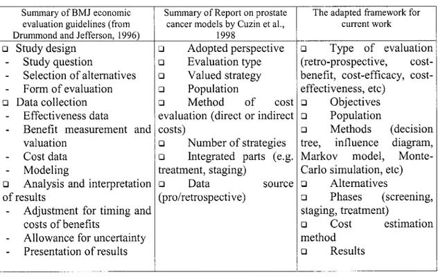
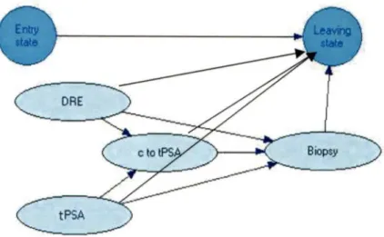
Figure 6 Schematic representation of the natural history of prostate cancer Figure 7 Beliefnetwork for "tPSA+DRE+c/tPSA+Biopsy" strategy Figure 8 Beliefnetwork for "tPSA+DRE+f/tPSA+Biopsy" strategy Figure 9 Beliefnetwork for "tPSA+DRE+Biopsy" strategy

Figure 10 Belief network for "cPSA+DRE +Biopsy" strategy Figure 11 Belief network for "cPSA+Biopsy" strategy Figure 12 Beliefnetwork for "tPSA+Biopsy" strategy Figure 13 Belief network for Phase 2 of the model Figure 14 State transition diagram for a model

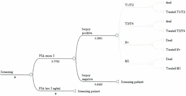
23 24 25 26 27 47 62 63 63 64 64 64 65 69 Figure 15 A fragment of decision tree represents screening, staging and treatment for one

particular alternative

Figure 16 Literature source dataset for DRE (screening and diagnosis phase)

70

74

Figure 17 Variability between probabilities for DRE among the studies vs. study size 75

Figure 18 Literature source dataset for tPSA (screening part) 78

Figure 19 Variability between tPSA probability among the studies vs. study size 78

Figure 20 Literature source dataset for positive bone scan 83

Figure 21 Variability between bone scan probabilities among the studies vs. study size 83 Figure 22 Literature source probability for a positive lymph nodectomy 85 Figure 23 Variability between positive lymph nodectomy probabilities

among the studies vs. study size

Figure 24 Simulation data histograms for screening alternatives (Monte-Carlo simulation, 1000 cycles)

Figure 25. Part of the model used for sensitivity analysis

Figure 26 Sensitivity analysis for probabilistic parameters in order to estimate influence on overall survival

86 95 99 100

List of Tables

Table 1. Current classifications of prostate cancer 10

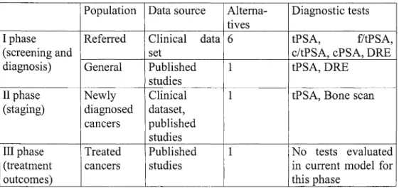
Table 2. Definitions and meaning of each attributes of chance nodes. 34 Table 3. Evaluation frameworks for decision modeling studies 39 Table 4. Keywords for a search in bibliographie databases 51 Table 5. Comparison between two decision modeling software 55 Table 6. Set of diagnostic procedures for different alternative screening strategies 61 Table 7. A summary of information about treatment groups 67 Table 8. Modeling approaches used for the three phases of building the mode! 71 Table 9. Summary about literature source for DRE (screening and diagnosis phase) 72 Table 10. Literature source dataset for DRE (screening and diagnosis phase) 73 Table 11. Summary about the literature sources for PSA screening 76 Table 12. Literature source dataset for PSA (screening part) 77

Table 13. Summary of literature sources for biopsy (screening and diagnosis phase) 79 Table 14. Literature source dataset for biopsy (screening and diagnosis phase) 79 Table 15. Summary of literature sources for bone scan staging 81 Table 16. Literature source dataset for bone scan staging 82 Table 17. Summary of literature sources for a lymphnodectomy 84 Table 18. Literature source dataset for a lymphnodectomy 85 Table 19. Summary about literature source for treatment options 87 Table 20. Demographic characteristics for Bayer clinical study dataset (referred patient

population) 88

Table 21. List of variables used for calculations (DRE + New_Test strategy) 90 Table 22. List of variables used for calculations ((DRE and/or PSA>4µg/l) + New_Test

strategy) 91

Table 23. Adjusted eut offs for biochemical test for alternative strategies Table 24. Probabilistic information from Bayer clinical study dataset Table 25. Details on costs for diagnostic procedures

Table 26. Expected utility for prostate cancer mode! Table 27. Alternative strategies comparison

Table 28. Summary about ail findings from the mode!

91 92 93 96 97 103 Table 29. Summary table on decision models on prostate cancer published between

Table 30. Summary table on decision models on prostate cancer published between

List of Abbreviations

ACS-NPCDP - The American Cancer Society- National Prostate Cancer Detection Project BMJ - British Medical Journal

CHUS - Centre Hospitalier de l'Université de Sherbrooke

cPSA (or cASP)- complexed prostate specific antigen (or l'antigène spécifique de la prostate complexe)

c/tPSA (or c/t ASP)- complexed-to-total prostate specific antigen ratio (or le rapport de ASP complexe sur ASP totale)

CT - computerized tomography

DRE (or TR)- digital rectal examination (or touché rectal)

ERSPC - European Randomized study of Screening for Prostate Cancer FN -false negative

FP - false positive

fPSA (or lASP)- free prostate specific antigen (or l'antigène spécifique de la prostate libre) f/tPSA (or l/t ASP) - free-to-total prostate specific antigen ratio (or le rapport de ASP libre

sur ASP totale) GS - Gleason Score

MRI - magnetic resonance imaging P AP - prostatic acid phosphatase PC - prostate cancer

PLCO - Prostate, Lung, Colorectal and Ovarian Cancer Screening Trial PSA (or ASP) - prostate specific antigen

QALE - quality adjusted life expectancy QAL Y - quality adjusted life year RCT - randomized clinical trial

ROC - receiver operating characteristics TN - true negative

TNM - American Joint Committee on Cancer's morphological classification TP - true positive

tPSA (or tASP) - total prostate specific antigen

(or l'antigène spécifique de la prostate totale) y.o. - years old

1.

Introduction

The subject of this master's thesis is the development of a decision model that concems the screening, staging and treatment phases of prostate cancer. This chapter starts with consideration of major evidence on the importance and characteristics of prostate cancer. This is followed by a discussion on decision modeling in health care. The modeling domain and clinical domain sections contain core information about the problem perspectives studied in relation to the developed model. The subsequent section provides different points of view on the use of information and evidence in health care decision making. The analysis of prostate cancer decision models published to date finishes the chapter.

Importance of prostate cancer

Prostate cancer is a growmg health problem with considerable econom1c consequences (VARENHORST et al., 1994). Prostate cancer is now the most common cancer and the second most common cause of death from cancer among men (NEHEMAN et al., 2001, RECKER and LUMMEN, 2000, WINGO et al., 1995). Radical treatment is usually possible for organ confined disease (NEHEMAN et al., 2001, RECKER and LUMMEN, 2000).

Han et al. (2001) have shown that a screening program for prostate cancer can improve diagnosis of early stages. Organ confined cancer is more frequent for cases identified by the screening program. They demonstrated a biochemical recurrence-free survival advantage due to an improved therapeutic outcome and lead time bias (HAN et al., 2001).

Populational impact of screening

Several publications exist in the research literature to investigate prostate cancer problem and the impact of screening, diagnosis and treatment. The studies differ by population and study design. The introduction of the prostate specific antigen screening test (PSA) and its impact on the subsequent management of disease has been increasingly studied. The impact of screening remains a centre of attention.

Sanna and Schottenfeld (2002) conducted a retrospective study linking demographic data from a US population with an implementation of prostate cancer screening in clinical practice. Prostate cancer incidence increased steadily from 1981 to 1989, with a steep increase in the early 1990s, followed by a decline. The exaggerated rate of increase in the early 1990s in prostate cancer incidence was transient and likely a result of increased detection of preclinical disease that was prevalent in the general population (SARMA and SCHOTTENFELD, 2002).

Results of two studies on the Quebec population were published in last five years. The conclusions derived from them illustrate the controversy about screening. Perron et al. (2002) did a retrospective study on birth cohorts of the Quebec province using regression modeling on relative mortality with factors including an exposure to prostate cancer screening. According to them, the difference in prostate cancer mortality is not attributable to total PSA (tPSA) screening. If tPSA screening is effective in preventing or postponing death from prostate cancer, its impact at a population level has yet to be felt. They suggested that there may be other explanations for the recent decline in prostate cancer mortality, consisting primarily of changes in disease management and in hormonal treatment of advanced disease (PERRON et al., 2002).

The second study, also from the Quebec population, shows another point of view. If tPSA screening is started at the age of 50 years, annual or biannual tPSA alone is highly efficient to identify the men who are at high risk of having prostate cancer. This prospective study was conducted on a population of men randomly allocated into screening and non-screening groups with ratio 2: 1. Patients were randomly selected from the electoral list and invited by mail without any public announcement. Labrie et al. ( 1999) demonstrated that early diagnosis and treatment permits a decrease in deaths from prostate cancer (LABRIE et al., 1999).

Vis (2002) summarized the study design critique of these two trials. In his view the reported decline may be the result of increased use of curative treatment before the implementing of tPSA screening and the availability of new treatment options for advanced prostate cancer. Changes in diet, lifestyle and environmental conditions, and the incorrect labeling of deaths from other causes could be also attributable (VIS, 2002). The scientific community is also waiting for the results of two ongoing randomized controlled trials in North America and Europe (European Study of Screening for Prostate Cancer (ERSPC)1 _and

Prostate, Lung, Colorectal and Ovarian Cancer Screening Trial (PLC0)2). These studies are supposed to provide the definitive evidence whether tPSA based screening is beneficial for patient survival or not. Results from these studies are expected to be available by 2006-2008.

Diagnostic problems in prostate cancer

There are other questions yet to be discussed which are relevant to the current screening programs. A prostate biopsy is an obligatory test to confirm the presence of prostate cancer. Screening programs are aimed to select appropriate groups of patients for

1 _{See hltQ_://www.crspc.o_i:gc . Accessed on the 19th of July 2004.}

prostate biopsy. Screening programs have low specificity, which cause 65-75 % negative biopsies for some groups of patients ( e.g. 4-10 mg/l range of prostate specific antigen, or tPSA) (POTTER et al., 2001). Roberts et al. (2000) supported the use of diagnostic techniques in order to reduce the number of negative biopsies and improve cancer yield in younger men. Repeated negative biopsies assumed as unnecessary might frustrate a patient if the screening program is provided on serial basis ( e.g. annually). It also has an influence on increase of health care costs (ROBERTS et al., 2000). This could give an explanation why serial screening programs are not commonly adopted.

Hence, despite the fact that prostate cancer is well represented in the scientific literature and is a problem with large impact on population health, grey zones are still left. Major tapies during the last 10 years after bringing tPSA screening into practice, were screening effectiveness, optimal use of screening markers and evaluation of measures of free or complexed PSA derivatives vs. total PSA.

Prostate cancer domain

This section provides a review of existing evidence for the prostate cancer domain, which is necessary for understanding the structural assumptions for the prostate cancer models.

Natural history of prostate cancer

In general it is a slow growing cancer (KESSLER and ALBERTSEN, 2003). Age is the most important factor associated with the cancer development (PORTER et al., 2002). For men between 40-49 years old a histological prevalence of the prostate cancer is near 12%, but for the men after 80 years old it is up to 43% (COLEY, 1997a). Near 95% of prostate cancers are adenocarcinomas. Most prostate cancer (75%) arises in the peripheral

zone of the prostate gland, nearly 15% develops in the transition zone and the remainder arises in the central zone (AUGUSTIN et al., 2003). Despite the fact that prostate cancer cells have been detected in almost 113 of men over 50, in many cases disease does not reach clinical stage (SCARDINO et al., 1989). A candidate for predicting risk of developing cancer is prostatic intraepithelial neoplasia (DEMARZO et al., 2003).

The prostatic capsule acts as an initial barrier to local invasion of the surrounding tissues. If localized within the prostate capsule, the cancer is assumed eligible for radical treatment using prostatectomy or radiotherapy, which is associated with a good prognosis. Once the capsule is invaded, the disease is viewed as locally advanced prostate cancer. Invasion of vascular and lymphatic tissue introduces the chance of metastatic spread of disease. Lymph from the prostate gland drains into lymph nodes in the pelvis, groin and lower back and these lymph nodes become common sites for metastasis. Secondary disease from prostate metastases mainly arises in the bones (FRYDENBERG, 1997).

Screening and diagnosis

Prostate cancer is usually described as induration of the prostate on digital rectal examination (DRE) if palpable (PRESTI, Jr. et al., 2000). The implementation of serum testing for tPSA has significantly improved the ability to detect cancer. tPSA used as pre-screening followed by DRE is highly efficient in detecting prostate cancer at a localized stage (CANDAS et al., 2000). While serum tPSA testing combined with DRE has good sensitivity for detecting prostate cancer, specificity is low due to the non-cancer specific elevation of tPSA, which is attributable to benign prostate disease (BRA WER, 2000).

Hoedemaeker et al. (2000) suggested that screening for prostate cancer leads to an increase in surgical treatment for relatively small tumors that have a higher probability of being organ confined. The frequency of positive lymph nodes at operation decreases

dramatically and the proportion of organ confined tumors after surgery increases, there is a shift from tumors with Gleason Score (GS) 8-10 towards lower grade tumors at radical prostatectomy (HOEDEMAEKER et al., 2000).

According to Candas et al.'s (2000) results from a cohort study of 11,811 participants, there is a 7-fold decrease in prevalence of prostate cancer at follow-up visits done up to 11 years. tPSA alone allowed to find 90.5% and 90% of cancers at first and follow-up visits, respectively, compared to 41.1 % and 25% by DRE alone. This means that tPSA is not losing performance due to eliminating cancer cases from the follow-up population (CANDAS et al., 2000). Rietbergen et al. (1998) also indicate that the chance of diagnosing prostate cancer in men by a positive DRE is decreased at follow-up visits in comparison to the first visit for serial screening program (RlETBERGEN et al., 1998).

PSA and derivates as screening markers

tPSA consists of 3 forms: free PSA, PSA complexed with alpha 1-antichymotrypsin and PSA complexed with beta macroglobulin (CHRlSTENSSON et al., 1993). The beta 2-macroglobulin bound form cannot be detected by monoclonal and polyclonal antibodies prepared against PSA. Of the 3 major serum forms of PSA, only free PSA and PSA complexed with alpha 1-antichymotrypsin are immunodetectable by current commercial assays (CATALONA et al., 1995, OESTERLING, 1995).

In the commonly accepted diagnostic zone of 4 to 10 µg/l total PSA, prostate cancer is present in 25% of patients. To maintain acceptable sensitivity a high number of biopsies are being performed. This tPSA range is often called a grey zone. Such patients are viewed by many researchers as a potential population where specificity of screening program could be improved (BRA WER et al., 2000). Several modifications to screening programs have been recently suggested like age-adjusted tPSA eut-offs, tPSA density (LENTINI et al.,

1997, PIZZOCCARO et al., 1994), tPSA adjusted for volume of transition zone (GUSTAFSSON et al., 1998, KIKUCHI et al., 2000, LUBOLDT et al., 2000, MAEDA et al., 1997). However none of these proposed approaches has gained common practice use (FLESHNER et al., 2000).

Several studies have demonstrated that the proportion of free or complexed-to-total PSA enhances the clinical usefulness of PSA testing for the early detection of prostate cancer, and it may reduce unnecessary biopsies (MILLER et al., 2001, MITCHELL et al., 2001, PRESTIGIACOMO and STAMEY, 1997, TANGUAY et al., 2002, VASHI and OESTERLING, 1997, WOODRUM, 1998). Complex-to-total PSA (c/tPSA) and free-to-total PSA (f/tPSA) ratio were found similar in performance (LEIN et al., 2001, OKEGAWA et al., 2000). Both of them can significantly improve detection of prostate cancer especially in the 4-10 mg/l tPSA range.

The normal reference range of free-to-total PSA ratio reported by Catalona et al.(1995) and Oesterling (1995) was 23 to 31 percent (CATALONA et al., 1995, OESTERLING, 1995). Percent of free PSA may increase the specificity of tPSA testing without sacrificing the cancer detection rate (HIGASHIHARA et al., 1996, WOODRUM, 1998). Brawer et al. (2000) further demonstrated that the complexed PSA method as a single measurement enhances specificity for detecting prostate cancer comparable to the measurement of percent free PSA. These findings suggest that complexed PSA may serve as a single assay replacement of the measurement of total PSA (BRA WER et al., 2000). Summarizing the presented evidence the order of biochemical markers as they were introduced into practice has been the following [ PSA (or PSA density)~ fPSA(or

Biopsy

Djavan et al. (2001) in a prospective study on prostate cancer detection with repeated biopsies for men with total PSA between 4 and 10 µg/l found a 10% cancer rate on second biopsy 6 weeks after a first negative biopsy. The initial cancer rate on the first biopsy was 22% (DJA V AN et al., 2001 ). These findings suggest that needle prostate biopsy is an imperfect test for determination of prostate cancer for a screened population. However this test is still the best available for the cancer detection. Currently second biopsy just after the first one to find missed cancers is not judged necessary. Sorne missed cancers (up to 10 -11 % ) might be diagnosed next year during a next round of the screening.

Trans-rectal ultrasound of prostate

Trans-rectal ultrasound of prostate (TRUS) is not warranted in men with normal DRE and tPSA results (BABAIAN et al., 1993). Various studies have suggested to avoid TRUS as the first order test (e.g. when selection of general population for prostate biopsy was done using three tests such as tPSA, DRE and TRUS independently) (HIGASHIHARA et al., 1996).

Serial prostate cancer screening

Most of the published studies show results on 1 year (or single measurement) screening. At any given visit, the tPSA levels of approximately 25% of men with initially elevated levels had decreased to less than 4.0 µg/l. Of all prostate cancer detected, 85% were detected during the first 2 years of screening. After 3 to 4 years of screening, the proportion of men with abnormal test results decreases substantially, the cancer detection rate decreases even more to approximate the expected prostate cancer incidence rate. There is a shift to detection of earlier-stage disease (SMITH et al., 1996).

Rietbergen et al. (1999) provides comparative evidence on the impact of prostate cancer screening. Comparison of the characteristics of prostate cancer between two populations (screening general population vs. population without screening) revealed reduction in advanced stage disease primarily due to the number of metastatic cases. Authors suggested further evaluation of stage reduction and disease specific mortality (RIETBERGEN et al., 1999).

Staging

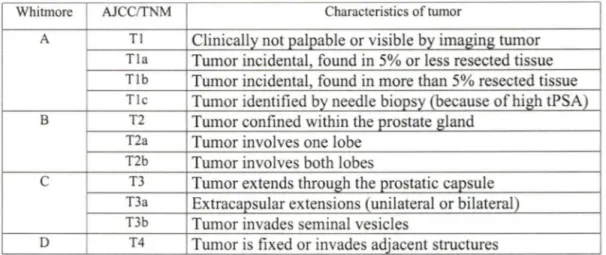
There are two main stage classifications of prostate cancer (TNM3 _{and Whitmore).} TNM is a way of describing the size, location and spread of a tumor. T denote the primary tumor according to its size and location. N refers to whether the cancer has spread to the lymph nodes that drain fluid from that area. M represents whether there are metastases in distant areas (e.g. Ml cancers) (STAMEY et al., 1998). Cancer development time consists of two stages "latent" and "clinical" cancer. Another classification was suggested by Whitmore. The correspondence between these two classifications is presented in Table 1.

Table 1. Current classifications of prostate cancer (FRYDENBERG, 1997, HAN et al., 2000, O'DOWD et al., 1997).

Whitmore AJCC/TNM Characteristics of tumor

A Tl Clinically not palpable or visible by imaging tumor

Tla Turnor incidental, found in 5% or less resected tissue

Tlb Tumor incidental, found in more than 5% resected tissue

Ti c Tumor identified by needle biopsy (because of high tPSA)

B T2 _{Tumor confined within the prostate gland} T2a Tumor involves one lobe

T2b _{Tumor involves both lobes}

c

T3a _{Extracapsular extensions (unilateral or bilateral)} T3b _{Tumor invades seminal vesicles}

D T4 _{Tumor is fixed or invades adjacent structures}

There is a continuous discussion on what should be viewed as latent and clinical cancers. In general the impact of presence of the cancer on the expected life length is the only parameter for assessing clinical significance. There is an increasing probability to die from other reasons with increasing age rather than to die from prostate cancer.

Detailed information about prostate cancer profile (stage distribution, age stratification, mo1tality) is very useful for an estimation of general impact on population health after tPSA implementation. Amling et al. ( 1998) have examined a large population (5,568 referred patients with prostate cancer, who underwent pelvic lymph nodectomy and radical retropubic prostatectomy between 1987 - 1995) who had adenocarcinoma of the prostate. The percentage of patients with stage Tl c prostate cancer (this stage can be detected by tPSA only) increased, and stage T3 cancer decreased. At the same time histological grade decreased and the proportion of pathological organ-confined disease increased, which is similar to clinical stage changes. Five-year progression-free survival was 85% and 76% for patients with clinical stage Tlc and T2, respectively. Radical prostatectomy experience has shown a significant migration to lower-stage, more differentiated, more often organ-confined

prostate cancer at the time of initial assessment after tPSA testing has appeared in clinical practice. Cancer-free survival associated with tPSA-detected cancer (Tlc) is superior to that with palpable tumors (T2). Due to study design limitations, Amling et al. (1998) also suggested that improved long-term cancer-specific survival remains to be confirmed with longer follow-up (AMLING et al., 1998).

Treatment selection is influenced by local stage assessment. Most of the time, clinicians must distinguish between pathologically (p) confirmed organ-confined disease (pTl-2) and non-confined disease (pT3-4) (PRESTI, Jr., 2000). Patients with organ-confined disease can be treated with surgery or radiation therapy, patients with extra capsular extension or seminal vesicle invasion are not surgery candidates. They can be treated with radiation therapy, hormonal therapy or a combination ofboth (YU and HRICAK, 2000).

Understaging may result in ineffective local treatment (surgery or radiation therapy) with the unnecessary risks and costs. Overstaging may result in withholding potentially radical therapy when a tumor might be amenable to definitive local treatment (KINDRICK etal., 1998).

Clinical stage

T stage is the clinical determination of local extension of disease primarily by digital rectal examination. The most widely used clinical stage classification system for prostate cancer was introduced by Whitmore. The clinical T stage only indirectly helps the urologist make important pre-treatment diagnostics decisions. DRE lacks specificity in the determination of organ confined (or sensitivity for non-organ confined) disease. But the predicted clinical stage correlates with pathological stage (ODOWD et al., 1997).

A prostate cancer preoperative stage underestimates the final pathology stage in approximately 40-50% of the cases (RUBIN et al., 1997). The frequency of pathologie

understaging is partly related to a clinical stage ranging from 30% in clinical stage Tl b to 60% in clinical stage T2 disease. Non-palpable (Tlc) prostate cancer is the most commonly diagnosed stage of disease at presentation today because of the widespread use of tPSA (PRESTI, Jr., 2000). Clinical stage is effective for identifying advanced disease. (YU and HRICAK, 2000).

Tumor grade (Gleason score)

The Gleason grading system is the most commonly used grading system for prostate cancer histology in North America. The pathologist assigns a primary grade to the pattern of cancer that is most commonly observed and a secondary grade to the pattern of cancer that is the second most commonly observed in the specimen. Grades range from 1 to 5. The Gleason score is obtained by adding the primary and secondary grades together. Well-differentiated tumors have a Gleason sum of 2 to 4, moderately Well-differentiated tumors have a Gleason score of 5 to 6, whereas poorly differentiated tumors have Gleason score of 8 to 1 O. The likelihood of having organ-confined disease decreases with increasing tumor grade (PRESTI, Jr., 2000).

PSA for preoperative stage determination and assessment of imaging needs

tPSA does not have perfect predictive capacity for a particular clinical stage. However total serum PSA correlates directly with advancing clinical and pathological stage of prostate cancer (PAR TIN et al., 1993). Imaging is quite an expensive procedure. tPSA has been used to identify the group of patients where imaging would be more efficient. Men with tPSA level less than 4 µg/l generally have organ-confined disease, whereas approximately 50% of patients with tPSA levels over 10 µg/l have extra-capsular extension. (PRESTI, Jr., 2000). According to Morote et al. 's (1997) study, tPSA can be successfully used to eliminate

the radionuclide bone scan in 40 % of patients with newly diagnosed prostate cancer (MOROTE et al., 1997).

Other methods for preoperative stage determination

Combination of significant clinical information was used by Partin et al. (1993) to create nomograms for prediction of pathological state and justify the imaging needs for prostate cancer patients. The purpose was to improve outcome prediction. Such predictive models can be used as a diagnostic test itself. It is a very "easy to use" method. Using a logistic regression modeling approach, Partin et al. (1993) demonstrated that total serum PSA, when combined with Gleason grade and initial clinical stage assessed during digital rectal examination (DRE), provided the best separation among pathological stages (e.g. capsule penetration, extra-prostatic spread, metastases at lymph nodes) compared to any univariate independent variable (PARTIN et al., 1993).

lmaging

The imaging studies are used to identify metastases and/or extra-capsular extension in men with newly diagnosed prostate cancer. This allows identification of patients for whom the definitive treatment will not provide additional survival advantages. Wide variations exist in the use of Gleason Score and serum tPSA in imaging studies. Physicians performed radionuclide bone scans, computerized tomography (CT) and magnetic resonance imaging (MRl) on many men with newly diagnosed prostate cancer as part of the initial stage evaluation to determine whether disease extends beyond the prostate capsule to pelvic lymph nodes or bone (ALBERTSEN, 2000).

Bone scan and computer tomography

Traditionally the radionuclide bone scan has been the comerstone of prostate cancer stage determination. Previous (before the "PSA era") widespread use of bone-scan imaging was certainly reasonable, even in asymptomatic patients (LEE and OESTERLING, 1997).

Although the risk of a positive bone scan increased with increasing state and grade, tumor stage and grade were poor predictors of positive bone scan according to results of the Gleave et al. (1996) study. Up to 4% of patients with clinically confined or well-differentiated to moderately well-differentiated tumors had positive scans (GLEA VE et al., 1996). Several studies on bone scan and CT suggest that these should only be ordered for men with newly diagnosed prostate cancer with tPSA greater than 20 µg/l or tPSA greater than 10 µg/l and Gleason scores 8 to 1 O. Such populations with higher risk of extra-capsular extension have positive yields greater than 10 % on bone scans (ALBERTSEN, 2000, LET AIEF et al., 2000). Several authors stated that pelvic CT and bone scans for the stage determination are not advocated for the patients with a tPSA level of less 20 µg/l (LEVRAN et al., 1995, LORENTE et al., 1999, STOKKEL et al., 1998). At the same time other authors suggested decreasing tPSA eut-off till 10 µg/l for asymptomatic, newly diagnosed patients (ATAUS et al., 1999, LEE and OESTERLING, 1997, O'DOWD et al., 1997).

Cross-sectional imaging with computed tomography has not proven to be very sensitive for evaluation of extra-capsular disease extension. The very low predicted rate of seminal vesicle invasion and lymph node metastasis determined by the combination of Gleason's score, clinical stage, and tPSA suggests that little benefit is obtained from cross-sectional imaging in patients with rather well-differentiated lesions and tPSA less than 10 µg/l (MANY AK and JA VITT, 1998). Yu and Hricak (2000) suggested that there is no

consensus and there is not enough evidence for guidelines for evaluation of local prostate cancer extent imaging (YU and HRICAK, 2000).

Pelvic lymph node dissection

Dissection of pelvic lymph nodes is the time-proven method for assessment of node involvement. It usually accompanies radical prostatectomy, and can be done independently (by laparoscopy or by mini-laparotomy) before radiotherapy, perineal prostatectomy or if the tPSA is more than 20 µg/l or if the cancer is poorly differentiated or there is clinically advanced local disease, or bath. The incidence of disease metastatic to lymph nodes correlates directly with clinical stage. Patients with a tPSA of 20 µg/l or more, Gleason score 8 or more and abnormal digital rectal examination have a high risk for lymph node metastases (PAR TIN et al., 1993, WOLF et al., 1993b ).

Pathological stage

The pathological examination of radical prostatectomies and pelvic lymph node specimens provides the most accurate description of the extent of disease available (ODOWD et al., 1997). This can suggest treatment modification in order to improve patient survival if cancer was understaged. According to some recommendations, preoperative lymph node examination can suggest that operation should be stopped before actual prostatectomy.

Treatment

The most important decision to be made in the patient with newly diagnosed prostate cancer is whether or not definitive treatment is necessary. Patients with clinical stage T3 disease are not generally considered surgical candidates, whereas patients with clinically localized disease are considered potential surgical candidates (YU and HRICAK, 2000).

Patients with prostate cancer localized to the pelvis without nodal or distant metastases can be treated with radiation therapy (FRYDENBERG, 1997).

Hormonal therapy is the mainstay of treatment when the patient has lymph-node metastases or disseminated metastases. Bilateral orchidectomy has been the standard treatment for testosterone reduction. Analogues of luteinising-hormone releasing hormone are commonly used for chemical castration and have equivalent effect to bilateral orchidectomy. A combination of medical or surgical castration and anti-androgen therapy can be used to black both testicular and adrenal androgen activity (FRYDENBERG, 1997).

Practice evaluation and decision making

These days clinicians are often guided by peer reviewed guidelines provided by trusted health institutions or professional boards. Guideline content is established by evaluation of best clinical practice results based on published studies in health care. Guidelines review diagnostic tests, treatment and management of disease options.

Common sense suggests that diagnostic technologies should be disseminated only if they are less expensive, produce fewer untoward effects and are at least as accurate as existing methods. They should eliminate the need for other investigations without loss of accuracy. Providing results, acceptable by clinical community, ideally reqmres a randomized controlled trial in which patients receive the new test or an alternative diagnostic strategy (GUYATT et al., 1986). Multiple evidence on the same subject is often accepted by the research community. However heterogeneity in study design can make it difficult to combine data from different studies.

Evaluation of diagnostic tests

Galen ( 1982) has suggested four levels for evaluation of laboratory tests. The first level is analytical evaluation of the laboratory test, followed then by diagnostic analysis with evaluation of sensitivity, specificity and receiver operating characteristics (ROC) curve. The third level is operational analysis with evaluation of outcome of positive and negative results and efficiency. The last level contains medical decision making analysis with evaluation of threshold probability, cost-benefit analysis and decision analysis modeling (GALEN, 1982).

Measuring diagnostic effectiveness (the second level in Galen's classification of levels from above) has become routine for implementation of every new test in clinical practice. Sensitivity is the ability of a test to correctly identify individuals who have a given disease or disorder. This is translated to a formula as: TP/(TP+FN), where TP is for true positive, FN is for false negative. Specificity is the ability of a test to correctly exclude individuals who do not have a given disease or disorder. This is translated into a formula as TN/(TN+FP), where TN is for true negative, FP is for false positive. The area under the ROC curve is defined by a curve of sensitivity and 1-specificity at various threshold values. ROC analysis is the dominant technique for evaluating the suitability of diagnostic techniques for real applications (METZ, 1978).

Mclntosh et al. (2002) highlighted problems associated with translating a potential screening biomarker from the laboratory to its use in patient care. Such application may require an algorithm or screening rule or even protocol for its application. Any practical screening algorithm must do so with strict controls on test specificity to avoid false-positive results, and unnecessary patient alarm and risk. The author also indicated the importance of longitudinal screening programs. Such programs, where prior tumor marker values and

trends are analyzed, improve the diagnostic performance over a single determination (MCINTOSH et al., 2002).

Even using a marker that can distinguish patients eligible or not eligible for specific intervention may not guarantee survival difference. Estimates of survival difference can be replaced by a surrogate end-point if the size and study period relevant to survival end-point is not realistic (SARGENT and ALLEGRA, 2002).

Study design for survival comparison has a major impact on study validity. To evaluate the hypothesis that a new diagnostic test or strategy is beneficial, randomized controlled trials with two arms are recommended (GUYATT et al., 1986). Running a RCT usually requires a lot of resources. Measuring survival advantage requires long follow-up studies. Repeat studies for every new diagnostic marker or therapeutic changes risk to be wasteful.

Benoit and Naslund (1997) suggested if men aged 50 to 70 years potentially benefit the most from tPSA screening this benefit would not be realized until these men are in their seventh and eighth decades of life (BENOIT and NASLUND, 1997). This study underlines the timeline aspect for studies on evaluation of cancer markers.

There are various heterogeneous approaches at all phases of prostate cancer management (from screening through pretreatment diagnostics to treatment outcome). No single clinical study is able to evaluate the various approaches for diagnostics (screening, staging) at the same time due to study population size limitations. There are also continuous needs for evaluation of new approaches. If a study has been conducted before, repetition seems to be not appropriate from a research point of view ( e.g. "reinventing the wheel", no innovation). Such repetitions are also not popular for economic reasons.

Modeling has been proposed as a less expensive way to evaluate different strategies before conducting real clinical studies, because using a modeling approach, the answer to research questions is based on integration of data collected from a number of well undertaken studies (KWOK et al., 2001, SIMPSON, 1994).

Decision modeling in health care

Graphs are a natural way for information representation. Graphical modeling for decision support is getting more widespread. Among all quantitative decision making methods, this approach is a way to think of and communicate on the underlying structure of the domain in question. lt also helps the researchers to focus on structure rather than calculations (SMYTH, 1997).

The structure of a graphical model clarifies the conditional independencies in the implied probability models, facilitating model assessment and revision (SMYTH, 1997). Presence of disease or any other condition in any step of a diagnostic protocol can be defined as a probability (value or distribution) (PAUKER and KASSIRER, 1980).

An ideal decision-analysis model includes all important available interventions and defines and discloses the analyst's time frame and outcome assessment perspective. The results can be monitored and, if necessary, adjustments can be made after completing the model if new evidence is available or due to other reasons (NIELSEN and JENSEN, 1999).

The basis for decision modeling is expected utility theory. Expected utility theory is suggested to evaluate choice of different patient oriented medical strategies (CLAXTON et al., 2001 ). This theory states that we should always choose an alternative that maximizes the expected utility (NIELSEN and JENSEN, 2000). According to Claxton et al. (2001) the choice of strategy and decision for clinical study design and practice evaluation should be based on expected utility. The authors have applied this theory for estimating the needs for

conducting additional research or acquiring additional information through assessmg uncertainty surrounding outcomes of interest (CLAXTON et al., 2001).

Decision analysis is best applied in decisions when other factors in addition to acquisition costs are important in determining overall intervention or diagnostics costs for several alternatives. Buxton et al. ( 1997) listed situations were modeling can be useful. They include a variety of data sources (evidence from trials, systematic reviews of trials) and possibility of application to different clinical settings (BUXTON et al., 1997).

So the decision maker should start the modeling project from the identification of alternative decisions and all factors which could influence the decision. Then probabilistic and outcome data should be identified according to the criteria suggested by the decision maker.

Adaptation of existing published models can be a good approach for decision-modelers. Fewer resources are necessary for this approach, since the underlying structure and variables have already been established. This approach focuses specifically on tailoring an existing model to meet specific needs. But models are often difficult to reproduce because they are not thoroughly described in the literature (an issue of transparency) (SANCHEZ and LEE, 2000). To be useful, prostate cancer treatment models must be based on acceptable structural assumptions, contain valid data and be understandable to clinical experts (SIMPSON, 1994).

Decision analysis modeling is an economically attractive method for practice evaluation that uses different sources of evidence to draw the conclusions about the new technologies or approaches used in health care.

Modeling principles

Decision trees and influence diagrams are two approaches for graphical modeling of decision problems. They offer different perspectives on the same problem using the same mathematical relationship. Each represents certain dimensions explicitly and can sometimes hide other dimensions from view. Influence diagrams detail well the relations among many parameters; decision trees show sequential paths and their branching. U sing the two views at the same time is helpful for understanding a decision model (HELF AND and PAUKER, 1997).

Elements of the decision model

The following elements are considered as necessary elements for a decision model: decision node, chance node and utility node. The decision (one or man y in the same decision model) is usually represented as a rectangular node. The decision nodes correspond to decision variables and represent alternative actions under the direct control of the decision maker. In the decision tree, the arcs leaving the decision node indicate the possible decisions available at this decision node. In the influence diagram, the alternative scenanos are described at the decision node, but not represented as arcs leaving the node.

The chance nodes (drawn as circles) correspond to chance variables, and represent events which are not under the direct control of the decision maker. Each chance node has outcomes associated with such an event. For the decision tree, the arcs leaving the chance nodes represent outcomes for every particular chance node. The numbers on the arcs leaving chance nodes are the probabilities of the outcomes to appear. In influence diagrams, the arcs connecting chance nodes represent conditional dependency between them. The absence of

the link between chance nodes means that there is conditional independence between events. The outcomes and probabilities for these outcomes to appear are hidden in underlying tables for every chance node. A conditionally independent chance node has a 1 *n table where n is

the number of outcome for a particular chance node. Multiple links from other chance nodes require hierarchical tables, e.g. a chance node with n outcomes is conditionally dependent of two other chance nodes, so the underlying table for this node will be k*m*n, where n is number of outcomes from a particular node, m and k are number of outcomes for these two

nodes, linked to the first one. All chance nodes in the influence diagram form a belief network. In the belief network probabilistic inference is estimated by the Bayesian equation (see Equation 2 in Chapter III). According to Nielsen and Jensen (1999), influence diagram is a belief network augmented with decision and utility node(s) (NIELSEN and JENSEN, 1999).

Belief (causal probabilistic or Bayesian) networks allow qualitative knowledge (structure of a problem) and quantitative knowledge, derived from case databases, expert opinion and literature to be exploited in the construction of decision support systems for diagnosis, treatment and prognosis (ANDREASSEN et al., 1999).

Decision tree

The decision tree is a graphical description of a sequential decision process. Evaluation begins at the terminal nodes and progresses backwards to the decision node. At each chance node, a value is a summary of the weighted average of the values of its possible outcomes. The strategy with the highest (or lowest) expected value is the strategy of choice. Each branch (or arc) leads to a terminal node. At terminal nodes the process stops, and the utility associated with a terminal state can be evaluated. Branches could lead to a chance node (usually represented as a circle), where the result of the event (e.g. test in Figure 1) is

uncertain. The arcs could also terminate at nodes that either represent additional decision or terminal events.

Figure 1. Example of the generic decision tree structure (symmetric)

1 1

Test 2

~---Alternative 1

Decision

: Test 1

:,

Altemative2

Outcorne 1

Outcorne 2

Outcorne 1

Outcorne 2

1

0

1

0

The order in which the nodes are traversed from left to right is the sequential order in which decisions are made and/or outcomes of chance events are revealed to the decision maker. Decision trees are easy to understand and easy to salve. If a variable is not relevant in a scenario, a mode! structure simply does not include it. Decision trees are symmetric if all alternatives have the same structure, or asymmetric, as shown in Figures l and 2. Use of decision trees is however usually limited to small problems due to the exponential growth of the representation. Conditional independence is not explicitly represented in decision trees (BIELZA and SHENOY, 1996).

Figure 2. Example of the generic decision tree structure (asymmetric) Outcomel

---

_______

~

:

Influence diagrams were introduced as a formalism to mode! decision problems with uncertainty (DITTMER and JENSEN, 1997). An influence diagram can be converted into a decision tree. This approach is also used for solving influence diagrams (QI and POOLE, 1995).

Influence diagrams serve as a powerful modeling tool for symmetric decision problems. When formulating a decision scenario as an influence diagram, a sequential ordering of the decisions variables is required. No barren (unconnected) nodes are specified by the influence diagram since they have no impact on the decisions (NIELSEN and JENSEN, 1999).

To illustrate influence diagrams an example is shown on Figure 3. It contains two decision nodes (rectangles) that represent a choice to obtain a diagnostic test or to prescribe a treatment. Test results (a chance node) depends on the real disease status. Depending on test results, different treatment options may be prescribed (a decision node "Treat").

The set of value nodes (drawn as diamonds) defines a set of utility functions, indicating the local utility for a given configuration of the variables in their domain. The total utility is the sum of the local utilities. ln the current example only one utility node is present. Utility is calculated on the basis of real disease status and treatment prescribed. The evaluation is performed according to the maximum (minimum) expected utility principle.

Figure 3. Example of influence diagram elements

Dcc1s1011 nodc: dCL ÎSl()ll altcrnatm.::s undcr cnns1dcrat1011 Obtain test Trcat \ aluc nmk: (same informat1011 as shnwn al the end hranches "r the tkcis1011 trec

Probab1l1st1c relat1<lnship m1ght cxist

Chanœ node· prnbabilistic runcl1011 ( s;1111e as for baycs1an hel1cfnet1\ork)

An influence diagram representation of a problem is specified at three levels (graphical, functional, numerical). At the graphical level, a directed acyclic graph4 _displays

decision variables, chance variables and information constraints. At the functional level, the structure of the conditional distribution is specified for each node. At the numerical level, the numerical details for the probability distributions and the utilities are specified. The size of an influence diagram graphical representation grows linearly with the number of variables.

Influence diagrams are intuitive to understand and encode conditional independence relations (BIELZA and SHENOY, 1996).

Influence diagrams are Jess user friendly than decision trees to represent asymmetric decision problems (NIELSEN and JENSEN, 1999).

Markov models

Markov models are useful when a decision problem involves repeated events and the timing of events is important. The mode! assumes that the patient is always in one of a finite number of states of health referred to as Markov states. Ail events of interest are modeled as transitions from one state to another. Each state is assigned a utility, and the contribution of this utility to the overall prognosis depends on transition from or the length of time spent in the state. The time horizon of the analysis is divided into equal increments of time (so-called Markov cycles). During each cycle, a patient may make a transition from one state to another or to itself. On the state-transition diagram each state is represented by a circle (see Figure 4). Arrows connecting two different states indicate allowed transitions. Arrows leading from a state to itself indicate that the patient may remain in that state in consecutive cycles. A state transition diagram can be easily transformed into a decision tree representation form (see Figure 5).

Figure 4. State-transition diagram of Markov model

The length of the cycle is chosen to represent a clinically meaningful time interval. The utility that is associated with spending one cycle in a particular state is referred to as the

incremental utility. Utility accrued for the entire Markov process is the total number of cycles spent in each state, each multiplied by the incremental utility for that state. The probability of making a transition from one state to another during a single cycle is called a transition probability. The Markov process is defined by the probability distribution among the starting states and the probabilities for the individual allowed transitions. A transition matrix can be represented by n*n transition probabilities where n is number of states. Absorbing states are states that the patient cannot leave (e.g. death, etc) (SONNENBERG and BECK, 1993). A transition probability can be expressed as a single value(direct way) or as a net probability (indirect way). If it is difficult to specify the transition directly, the net probability can be modeled using chance nodes and the probabilistic influences among them (LEONG, 1998).

Figure 5. Decision tree representation of Markov model

Current State Statel 1.0 Current S tate State2 0.0 Next State Statel 0.0 Next State State2 1.0 Next State Statel 0.0 Next State State2 1.0

Two different types of Markov model can be characterized by the form of the transition probabilities. A special type of Markov process in which the transition probabilities are constant over time is called a Markov chain. This has distinct analytical advantages since the probability of being in a particular state at a particular point in time can be calculated simply by raising the transition matrix to the power of the appropriate cycle. The more general Markov models, where transition probabilities can vary over time, are known as a time-dependent Markov process (BRIGGS and SCULPHER, 1998).

An important limitation of the Markov model is that the probability of moving out of a state is not dependent on the states a patient may have experienced before entering that state (so-called Markovian assumption) (BRIGGS and SCULPHER, 1998).

The accuracy of Markov model results depends on the accuracy of the estimates for the transition probabilities between different states of the model. They could be derived from cohort studies, which however could be subject to selection bias. The precision of an estimate is directly related to the number of person-years of observations for the cohort. The model uses inputs such as the probabilities of eventually dying with different stages of disease (absorption probabilities) or the mortality rates from other causes (BLACK et al., 1997).

Dynamic influence diagrams

Leong (1998) published a work on representation and solving clinical problems as dynamic influence diagrams. In a dynamic influence diagram, similar elements to other modeling approaches can be found. The dynamic influence diagram has decision nodes, chance nodes and the value nodes (like influence diagrams) and also state variable nodes. Arcs between chance nodes represent conditional dependence (LEONG, 1998).

This researcher has made an analysis of dynamic decision modeling approaches and developed an integrated decision language (DynaMoL) with four components (dynamic decision grammar, graphical representation convention, the mathematical representation and a set of general translational techniques). She has also implemented this language in a prototype and described several medical domain problems. The prototype has been further developed in a software application for decision analysis modeling ("ReasonEdge Modeler"). This software has 3 views of a model structure. The state transition diagram represents all states of the model, which can influence expected utility. Links between different states

represent allowed transitions of patients between states. Utility is referenced to "being in the state" or as "transition from one state to another". Transitional probability can be represented as a beliefnetwork or decision tree (LEONG, 1998, LEONG and CAO, 1998).

The author has shown the DynaMoL framework as a platform for automatic derivation for numerical parameters, supporting knowledge based model construction and automated knowledge acquisition from multiple knowledge sources (CAO et al., 1998, CAO and LEONG, 1997, LAU and LEONG, 1999, WANG and LEONG, 1998).

Mode! evaluation

Structural level

Evaluation of a model starts from the evaluation of how the model structure represents the clinical problem. The clinical problem can be described as a text or represented graphically. In decision modeling each node represents some kind of event or diagnostic test. The decision model should contain a necessary set of elements to represent the clinical problem and to answer research questions.

Functional Level

Links between chance nodes represent the nature of the relationship between the events. The conditional dependency can be visually evaluated with a belief network. The same task becomes difficult when only a decision tree representation of the decision model is used. The conditional dependencies between chance nodes are hidden behind the numbers on the branches that emanate from these chance nodes. Decision model alternatives represent scenarios relevant to clinical practice.

Briggs (2000) recognized three categories of uncertainty, which could be generally applied to the numeric level:

1) uncertainty relating to observed data inputs. Typically, confidence intervals might be presented, the size of which depends not only on sample size, but also on within sample variability;

2) uncertainty relating to extrapolation. This includes data generalized from other settings, as well as data modeled using epidemiological models or regression;

3) uncertainty relating to data analytic methods.

To deal with these sources of uncertainties, careful selection of numeric information should be done in order to specify the probabilistic relationship between events (BRIGGS, 2000).

The accuracy of a decision model depends on the accuracy of the estimates for the transitional and conditional probabilities used in the model (BLACK et al., 1997). Transition between Markov states is defined by the logical temporal relationship between conditions of the patient represented as Markov states (e.g. no transition from state "Dead" to state "Alive").

If a transitional probability is not available, the parameter might be estimated through conditional probabilities using a belief network. For example, transitional probability between state 1 (e.g. "healthy patient" ) and state 2 (e.g. "disease") is unknown. But the model developer could estimate the probability of developing the "disease" if patients were exposed to some factor, and the prevalence of this factor in the population is known. Transitional probability is calculated using the Bayesian equation (see Equation 2 in Chapter III). A belief network for transitional probabilities can be useful also for conducting