Les Cahiers de la Chaire Economie du Climat
Will technological progress be sufficient to effectively
lead the air transport to a sustainable development in
the mid-term (2025)?
approach
Benoit Chèze
1, Julien Chevallier
2and Pascal Gastineau
3The aim of this article is to investigate whether anticipated technological progress can be expected to be strong enough to offset carbon dioxide (CO2) emissions resulting from the rapid growth of air transport. Aviation CO2 emissions projections are provided at the worldwide level and for eight geographical zones until 2025. Total air traffic flows are first forecast using a dynamic panel-data econometric model and then converted into corresponding quantities of air traffic CO2 emissions, through jet fuel demand forecasts, using specific hypothesis and energy factors. None of our nine scenarios appears compatible with the objective of 450 ppm CO2-eq. (a.k.a. “scenario of type I”) recommended by the Intergovernmental Panel on Climate Change (IPCC). None is either compatible with the IPCC scenario of type III, which aims at limiting global warming to 3.2◦C. Thus, aviation CO2 emissions are unlikely to diminish over the next decade unless there is a radical shift in technology and/or travel demand is restricted.
Keywords: Air transport; CO2 emissions; Forecasting; Climate change. JEL Classification Numbers: C53, L93, Q47, Q54.
n° 2012-07
Working Paper Series
1. IFP Energies nouvelles, 1-4 avenue de Bois-Préau, 92852 Rueil-Malmaison, France. EconomiX–CNRS, University of Paris Ouest, France
Climate Economics Chair, Paris, France.
benoit.cheze@ifpen.fr
2. Université Paris Dauphine (CGEMP/LEDa), France EconomiX–CNRS, University of Paris Ouest, France
julien.chevallier@dauphine.fr 3. Ifsttar (LTE), Lyon, France.
EconomiX–CNRS, University of Paris Ouest, France
Will technological progress be sufficient to effectively
lead the air transport to a sustainable development in
the mid-term (2025)?
∗
Benoît Chèze
† ‡ §, Julien Chevallier
¶ ‡, and Pascal Gastineau
k ‡April 12, 2012
Abstract
The aim of this article is to investigate whether anticipated technological progress can be expected to be strong enough to offset carbon dioxide (CO2) emissions resulting
from the rapid growth of air transport. Aviation CO2 emissions projections are provided
at the worldwide level and for eight geographical zones until 2025. Total air traffic flows are first forecast using a dynamic panel-data econometric model and then converted into corresponding quantities of air traffic CO2 emissions, through jet fuel demand forecasts,
using specific hypothesis and energy factors. None of our nine scenarios appears com-patible with the objective of 450 ppm CO2-eq. (a.k.a. “scenario of type I”) recommended
by the Intergovernmental Panel on Climate Change (IPCC). None is either compatible with the IPCC scenario of type III, which aims at limiting global warming to 3.2◦C.
Thus, aviation CO2 emissions are unlikely to diminish over the next decade unless there
is a radical shift in technology and/or travel demand is restricted. Keywords: Air transport; CO2 emissions; Forecasting; Climate change.
JEL Classification Numbers: C53, L93, Q47, Q54.
∗The authors are grateful to the Lunch-Seminar’s participants (2011, April) of the Economics Department
of IFP Energies nouvelles (IFPEN). The authors also thank for their helpful comments L. Meunier (ADEME) and from the IFPEN: E. Bertout, P. Coussy, P. Marion, A. Pierru, J. Sabathier, V. Saint-Antonin, S. Tchung-Ming and S. Vinot. The usual disclaimer applies.
†Corresponding author. IFP Energies nouvelles, 1-4 avenue de Bois-Préau, 92852 Rueil-Malmaison, France.
benoit.cheze@ifpen.fr.
‡EconomiX–CNRS, University of Paris Ouest, France. §Climate Economics Chair, Paris, France.
¶Université Paris Dauphine (CGEMP/LEDa), France; julien.chevallier@dauphine.fr. kIfsttar (LTE), Lyon, France; pascal.gastineau@ifsttar.fr.
1
Introduction
This article proposes a discussion about the future evolution, until 2025, of carbon dioxide (CO2) emissions from the air transport sector. Besides, it analyses whether technological progress would be sufficient to outweigh growth in fuel use, and lead to either absolute or even relative CO2emission reductions. As shown in Figure 1, the share of CO2 emissions com-ing from air transport in total CO2 emissions linked to burning fossil fuels has been increasing from 2% in 1980 to 2.5–2.7% in 2007, i.e. an increase by 25% in less than thirty years. This evolution seems to have slowed down during the last decade (Figure 1 (a)). However, this slower pace cannot be associated with decreasing CO2 emissions coming from air transport, which have been steadily increasing from 350 Mt in 1980 to 750 Mt in 2007. Instead, it is due to an even stronger increase of the total CO2 emissions linked to burning fossil fuels (Figure 1 (b)). 0 0.5 1.0 1.5 2.0 2.5 3.0 1980 1984 1988 1992 1996 2000 2004 Sha re of C O2 emi ss io ns fr om ai r tr ans p or t in to ta l C O2 emi ss io ns 0 5000 10000 15000 20000 25000 30000 1980 1984 1988 1992 1996 2000 2004 0 1000 2000 C O2 emi ss io ns fr om ai r tr ans p or t (M t) T ot al C O2 emi ss io ns li nk ed to bur ni ng fo ss il fue ls (M t)
fossil fuels air transport
(a) (b)
Figure 1: Evolution of the share of CO2 emissions coming from air transport in total CO2 emissions linked to burning fossil fuels (graph (a)) as well as CO2 emissions coming from air transport (graph (b), right axis) and total CO2 emissions linked to burning fossil fuels (graph (b), left axis) from 1980 to 2007.
Source: Authors, from IEA data.
As a first conclusion, and even if Figure 1 does not take into account all greenhouse gases (GHG) emissions1, the current contribution of the air transport sector to climate change may
1
CO2 is one of the six gases whose anthropic origin is recognized by the UN Framework Convention on
Climate Change adopted by the Rio Summit in 1992. Other greenhouse gases include CH4, N2O, and fluorized
be seem as quite marginal. This statement shall not be misleading, and yield to undermine the risks associated with a continuous growth of the demand for air transport in the near future. At least for two reasons. First, Figure 1 shows only the CO2 emissions coming from air transport. There are other greenhouse gases associated with this activity, such as H2O and NOX, which have important climatic impacts2. Second, it is not negligible if we include the environmental risk attached to a sustained growth for the demand in air transport, which urges to take action. This sector indeed is growing very quickly, and the share of its emissions is steadily increasing (Figure 1). In 1999, the special report on air transport by the IPCC estimated that this sector could be characterized by a growth of its CO2 emissions comprised between 60% and more than 1000% from 1992 to 2050 (IPCC, 1999). Along with increasing environmental pressures, this future development of the aviation sector may be seen as un-sustainable.
That is why policy makers are more and more concerned by the future evolution of air transport, especially in Europe, and aim at limiting its CO2 emissions (Rothengatter, 2010, Zhang et al., 2010). Against this background, the international climate negotiations aim at reducing GHG emissions as much as possible, and compatible with the objective of limiting global warming by +2◦C (degrees Celsius) compared to the pre-industrial era3. To comply with this objective, the EU Commission has established in April 2009 the target to reduce greenhouse gases emissions by 20% in 2020 in its “Energy-Climate” Package. These reduction objectives are binding, and will also concern civil aviation with its inclusion in the EU ETS4. To sum up, policy makers distinguish between two kinds of measures to limit the
environ-2
For instance, H2O and NOX emissions produce ozone. The Intergovernmental Panel on Climate Change
(IPCC, 1999) estimates that these gases represent between 50% and 80% of the potential of global warming linked to aviation. However, these gases are difficult to quantify, since they vary depending on the type of flight. Besides, by their very nature (such as NOX which are indirect gases for instance), their impacts on the
climate depend on the location and the length of the emissions, and are not well understood by the scientific community to date. The IPCC therefore cautiously multiplies by a factor of two the CO2 emissions coming
from air transport in order to account for the total CO2emissions of this sector, which are then expressed in
CO2equivalent gases (CO2-eq.). 3
Since the Copenhagen COP/MOP Meeting in December 2009, the scientific objective has indeed been set to +2◦C. Recall that to achieve this +2◦Ctarget of limiting global warming, the IPCC suggests to decrease GHG emissions in industrialized countries by 25% to 40% in 2020, and by 80% to 95% in 2050 compared to 1990 levels (IPCC, 2007a, 2007b, SEG, 2007).
4
As of 2012, airline companies traveling in the EU must limit their CO2 emissions to 97% of the annual
mean recorded between 2004 and 2006. The airplanes taking off and landing in the EU 27, as well as coming from other countries, will fall under this regulation.
mental impact of the growth of air transport. The first one consists in improving the energy efficiency of aircrafts (and thus to lower their carbon intensity) by promoting technological innovation. The second one consists in binding measures dealing with the demand for air transport5. These two types of measures are not antinomic and may be pursued simultane-ously. For instance, the European Commission actively promotes innovation efforts by air companies through Research & Development (R&D) programs6, while also taking binding actions with the inclusion of aviation in the EU ETS. However, these public policies do not follow the same logic. Indeed, the latter kind of measure deals directly with the causes of greenhouse gases emissions linked to the growth of the air transport sector, while the former kind of measure only attempts at diminishing its negative consequences.
There is a sharp debate today on the best course of action to reduce significantly, and within a reasonable time horizon, greenhouse gases emissions in the air transport sector. Will technological changes7 be sufficient to outweigh growth in fuel use? In other words, shall we solely aim at reducing the carbon intensity of the air transport sector through innovation? Or shall we admit that technological innovation alone does not allow to achieve the objectives of stablization and reduction of greenhouse gases that were set? In both cases, shall we limit the development of the air transport sector?
The actors in the aeronautical industry tend to reject majoritarily the second kind of measure. For instance, concerning the inclusion of the air transport sector in the EU ETS, governments and international airlines outside Europe protest against this measure. Oppos-ing states (includOppos-ing Brazil, the U.S., China, and Japan) claim that the unilateral application of the EU ETS to international aviation violates the ‘cardinal principle of state sovereignty’, and assert that non-EU aircraft operators should be exempt from this trading scheme.
Aero-5
To be more precise, there are actually four general types of mitigation-related measures: climate policy, behavioural change, management and new technologies. All of these, with the exception of behavioural change, are supposed to contribute to efficiency gains in the aviation sector. Behavioural change, on the other hand, is supposed to make a contribution through low carbon choices (shorter flight distances, more environmentally pro-active airlines, direct flights, etc.).
6
Two main projects are devoted currently to alternative fuels (other than jet fuel) for aviation. The program Alfa-Bird, which was created in 2008 for a period of four years and coordinated by Airbus, aims at better identifying the needs in terms of research and investments. The Swafea program, lead since January 2009 by the French Aerospace Lab, aims at elaborating a roadmap for deploying alternative fuels in the mid-term. Many industrial actors (Airbus, Avio, Dassault, EADS, Rolls-Royce, Safran, Sasoil, Shell, Snecma, etc.) are participating to these programs, along with public research centers.
7
nautical industrials argue that there have been considerable advances in the carbon intensity of aircrafts since the start of the 1990s. Arguably, energy efficiency gains due to technological progress and the enhancement of the Air Traffic Management (ATM) have largely limited the impact of the growth of the air transport sector on the growth of greenhouse gases emisssions. They claim that technological innovation through R&D expenditures should be sufficient to stabilize and then reduce greenhouse gases. For instance, the Advisory Council for Aero-nautics Research in Europe (ACARE) has announced its will to develop by 2020 aircrafts emitting two times less CO2 emissions than aircrafts commercialized in 2000. The Interna-tional Civil Aviation Organization (ICAO) is asking its members to reduce on average by 2% per year their consumption of jet fuel until 2020. The International Air Transport Association (IATA), which concentrates 90% of airline companies, has declared that it will enhance the energy efficiency of its aircraft fleet by 25% in 2020, i.e. by 1.5% per year on average. To meet these objectives, airline companies advocate that many technological options exist in the near future such as lighter aircrafts, enhanced design, enhanced engines’ consumption, better traffic management, and replacing jet fuel with alternative fuels (bio-fuels) up to 10% in 2017. This article aims at evaluating whether the solutions proposed by the air transport indus-try can adequately reduce the GHG emissions coming from this sector. To do so, forecasts of CO2emissions from the air transport sector are performed based on various scenarios of evolu-tion of the energy efficiency of aircrafts (and others). We propose to examine more especially whether only technological innovation is able to effectively reduce the impact of air traffic on the growth of greenhouse gases. Technological innovation appears indeed central to tackle this environmental challenge. Arguably, the reduction of the carbon intensity of the fleet has strongly contributed to limit the impact of the growth in the air transport sector in terms of CO2 emissions. However, these emissions have been steadily increasing over the last thirty years (see Figure 1). Besides, we may observe that the growth of air transport has always been higher than energy efficiency gains over the last thirty years, so that CO2 emissions associated with this sector have also increased overtime. Despite the ambitious objectives in terms of energy efficiency gains put forward by the main stakeholders in the aviation industry, it is not straightforward that technological innovation alone will be able to annihilate the adverse environmental impacts of air transport. Evaluating whether the industrial policy proposed by the aviation industry will be enough to stabilize GHG emissions constitutes an important step to guide decision making in the public policy process. At the European level, such an evaluation is a pre-requisite to develop a coherent environmental policy in terms of reducing GHG emissions. If the current policies do not appear as sufficient, then additional binding
measures such as the inclusion of the air transport sector in the EU ETS since january 2012 would appear well-founded despite the claims by aeronautical industry8.
The analysis proceeds in two parts. Various projections of CO2 emissions in the air transport sector are presented (Section 2) and then compared with the literature (Section 3). The CO2 emissions projections presented below are deduced from forecasts of jet fuel demand presented in Chèze et al. (2011)9. Compared to the latter paper, the present article goes one step further by providing original projections of CO2 emissions in the air transport sector. It allows then to investigate whether or not technological innovation would be sufficient to lead to CO2 emission reductions based on various robustness checks.
Section 2 details our benchmark scenario, along with a sensitivity analysis based on eight alternative scenarios. The general methodology followed in Section 2 may be summarized into three steps. First, total air traffic flows (freight + passengers) and their growth rates (per year) have to be forecast by using dynamic panel-data econometric models. Second, these air traffic forecasts are converted into corresponding quantities of jet fuel using specific energy coefficients and traffic efficiency improvements hypothesis. Third, air traffic CO2 emissions are directly deduced from jet fuel demand forecasts by using the energy factor mentioned above (one kilogram of jet fuel – Jet-A1 or Jet-A – consumed emits 3.156 kilograms of CO2, recall footnote n◦9). According to our benchmark scenario (sc. A.1., see Figure 4), air traffic CO2 emissions should rise at a mean yearly growth rate of 1.9%. Driven by gross domestic product (GDP) growth, air traffic should sharply increase (4.7%/year), along with the asso-ciated demand for jet fuel (by taking into account energy efficiency improvements). Besides, none of the scenarios anticipates a decrease, or even a stabilization, of CO2emissions in the air transport sector by 2025 (although our benchmark scenario includes strong energy efficiency gains). Section 3 first compares the results obtained with both (i) the projections obtained in the academic literature and by the aeronautical sector and (ii) the SRES scenarios by the
8
The inclusion of aviation in the EU ETS ultimately aims at modifying the behaviour of economic agents. However, the current set-up of the system should not lead to absolute emission reductions, and possibly not even to relative emission reductions.
9
The CO2 emissions associated with air transport are directly linked to the quantity of jet fuel used by
the aircraft fleet. Once completely oxydized, one kilogram of jet fuel (Jet-A1 or Jet-A) consumed emits 3.156 kilograms of CO2. By applying this energy factor to the quantity of jet fuel used, it is readily possible to
deduce the CO2 emissions coming from the air transport sector. Note that this emissions factor is officially
used by the European Commission to account for the CO2 emissions from the aviation sector towards its
inclusion in the European Union Emissions Trading Scheme (EU ETS) by 2012 (see Amendment C(2009) 2887 completing the Directive 2009/339/CE and the Decision 2007/589/CE).
IPCC (Nakicenovic and Swart, 2000; IPCC, 2007a, 2007b)10. The latter comparison aims at evaluating whether our CO2 projections concerning the air transport sector are compatible with a growth rate yielding to a maximum limit of global warming to +2◦C compared to the pre-industrial era (IPCC, 2007a, 2007b). Finally, Section 4 concludes.
2
World and regional air traffic CO
2emissions projections
until 2025: Benchmark scenario and sensitivity analysis
This Section presents various forecasts of CO2 emissions coming from air transport by 2025. These forecasts are deduced from preliminary forecasts of jet fuel demand presented in Chèze et al. (2011). We follow thoroughly here the methodology developed by Chèze et al. (2010), which can be summarized as follows. The amount of CO2 emitted by an airplane may be deduced directly from the quantity of jet fuel consumed. Jet fuel is only used as a fuel in the aviation sector. Consequently, the consumption of jet fuel depends very closely on the demand for mobility for this transportation means. To understand the evolution of this consumption, we must start by studying the fundamentals of air transport. This task may be decomposed into three distinct steps. First, we perform various forecasts for air traffic in the mid-term (2025), at the world and regional levels. These forecasts are derived from the prior modeling and estimation of the relationship between air transport and its main determinants. This first step relies on econometric methods. Second, the data on air traffic are converted into corresponding quantities of jet fuel based by using energy coefficients11. Third, we deduce from the two preceding steps the CO2 projections for the air transport sector until 2025. This third step is simple to compute. Indeed, carbon dioxide constitutes with water vapor the main rejection of the jet fuel combustion in the atmosphere. These emissions are directly linked to the quantity of jet fuel used, i.e. burnt in order to power an aircraft, by using the CO2 emissions factor of 3.156 (recall footnote n◦9)12.Before presenting our scenarios of future evolution of air traffic CO2 emissions, this Section
10
These scenarios have been developed in a special report published by the IPCC (Nakicenovic and Swart, 2000) abbreviated as “Special Report on Emission Scenarios”.
11
Energy coefficients – as well as their evolution through time, i.e. energy gains – constitute one of the main assumptions of this work, as explained below.
12
Note that using this emissions factor does not allow to estimate all emissions of greenhouse gases from the air transport sector, but only the emissions coming from carbon dioxide.
begins by summarizing air traffic and corresponding jet fuel demand forecasts obtained by Chèze et al. (2010, 2011). Their results mostly depend on two broad hypotheses. The first one concerns the future evolution of economic activity in the various regions (estimated from regional GDP growth indicators). The second hypothesis deals with the energy efficiency coefficients that have been chosen to conduct the analysis, as well as their evolution overtime (i.e. energy efficiency gains). Thus, we present the CO2 emissions projections obtained in our benchmark scenario, and then we evaluate the robustness of these results obtained depending on these two broad hypotheses.
This modeling, and the associated forecasts, are applied to eight geographical zones and at the world level (i.e. the sum of the eight regions) by specifying a dynamic model on panel data. Air traffic forecasts are computed for the following regions: Central and North America, Latin America, Europe, Russia and Commonwealth of Independent States (CIS), Africa, the Middle East, Asian countries and Oceania (except China). The eighth region is China, in order to have a specific focus on this country. By doing so, this article proposes an analysis of potential future trends of air transport CO2 emissions, both at the world and regional levels, as a simple analysis of the future yearly mean growth rates of world air traffic emissions may mask a wide heterogeneity between geographical zones.
2.1
Forecasting air traffic until 2025 . . .
Air traffic projections are estimated by using econometric methods based on the historical relationship between air traffic and its main drivers (Chèze et al., 2010). Air traffic projec-tions proposed are obtained by using ICAO’s air traffic data13 during 1980-2007. According to the literature14, the air traffic drivers are mainly (i) GDP growth rates, (ii) ticket prices, (iii) alternative transport modes (such as train) and (iv) some external shocks such as the September 11th terrorist attacks in 2001. Last but not least, the magnitude of these drivers appears to depend on the maturity of the transport market: the growth rates of the domestic markets of industrialized countries are lower than those of emerging countries for instance, ceteris paribus. To take into account the latter criteria, the econometric modeling proposed
13
The “Commercial Air Carriers - Traffic” database of the ICAO provides air traffic for both cargo and passenger traffic. These data are both expressed in Revenue Tonne-Kilometre (RTK), so that they can be re-aggregated together. A Revenue Tonne-Kilometre denotes one tonne of load (passengers and/or cargo) transported one kilometre.
14
See in particular DfT (2009), ECI (2006), Eyers et al. (2004), Gately (1988), IPCC (1999), Macintosh and Wallace (2009), Mayor and Tol (2010), RCEP (2002), Vedantham and Oppenheimer (1994, 1998), Wickrama et al. (2003).
by Chèze et al. (2010) is carried out by using dynamic panel-data models for the eight geo-graphical zones15.
Based on assumptions on the evolution of the main drivers, Chèze et al. (2010) obtain different air traffic forecasts scenarios. These air traffic forecasts rely on a crucial assumption: the future evolution of the eight geographical regions’ GDP growth rates. Their Baseline air traffic forecast scenario, i.e. the “IMF GDP growth rates” scenario (see Figure 4), relies in particular on the International Monetary Fund (IMF) previsions of these GDP growth rates until 2014. Two other air traffic forecast scenarios are defined to measure the sensitivity of air traffic to changes in GDP growth rates: (i) in the “Low GDP growth rates” air traffic forecasts scenario, the IMF GDP growth rates are decreased by 10%, (ii) in the “High GDP growth rates” air traffic forecasts scenario, the IMF GDP growth rates are increased by 10% (see also Figure 4).
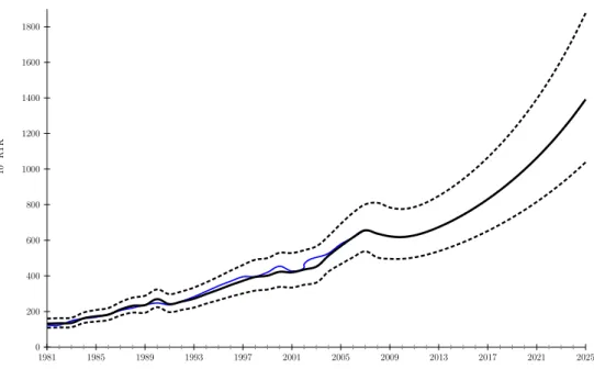
Figure 2 provides a visual representation of the Baseline air traffic forecasts scenario at the world level until 2025 (bold line, from 2008 to 2025) and their 95 % Interval Predic-tions16 (dashed lines, from 2008 to 2025). According to this scenario, this model predicts first a relatively high decrease of air traffic in 2008 and 2009 (- 3.47% between 2007 and 2008) followed by the recovery of its positive evolution from 2010 to 202517. World air traffic should, overall, increase at a yearly mean growth rate of 4.7% between 2008 and 2025, rising from 637.4 to 1391.8 billion RTK (see also Table 2). These air traffic forecasts differ from one region to another. At the regional level, RTK yearly average growth rates range from 3% per year in Central and North America to 8.2% per year in China (Table 2, first two columns). Air traffic forecasts obtained by Chèze et al. (2010) are not further commented here. These air traffic forecasts are necessary to deduce (i) the associated jet fuel demand (Chèze et al., 2011) which yields to (ii) the corresponding CO2 emissions by 2025 (i.e. what is developed in this article). The latter step is presented in the next Section.
15
The influence of the main air traffic determinants is estimated by using the Arellano-Bond estimator. GDP appears to have a positive influence on air traffic, whereas the influence of the jet-fuel price - above a given threshold - is negative. Exogenous shocks may also have a (negative) impact on air traffic growth rates.
16
Variance of in-sample predicted values and forecasts are different. As is intuitive, the variance of the forecasts is higher than the variance of the predicted values. This explains the progressively increasing gap between the lower bound and the upper bound of the 95 % Interval Predictions.
17
Negative GDP growth rates in 2008 and 2009 (according to IMF GDP projections) mainly explain the predicted decrease of air traffic during this period (See Chèze et al. (2010) for more details).
0 200 400 600 800 1000 1200 1400 1600 1800 1981 1985 1989 1993 1997 2001 2005 2009 2013 2017 2021 2025 1 0 9R T K
Blue line: ICAO data; bold line: in-sample predicted values (from 1981 to 2007) and air traffic forecasts (from 2008 to 2025); dashed lines: 95 % Interval Prediction.
Figure 2: World air traffic forecasts – expressed in RTK (billions) – until 2025 (Baseline scenario).
Source: Chèze et al. (2010), ICAO data.
2.2
. . . and corresponding aviation CO
2emissions
This Section presents various CO2 emissions scenarios of air traffic until 2025, both at the world and regional level. Recall that these scenarios correspond to CO2 emissions from Jet-A1 fuel. It is thus necessary to first obtain jet fuel demand forecasts. Once this step has been performed, one can readily deduce the amount of air traffic CO2 emissions by applying an emission factor equal to 3.156. As this last step computationally simple, it has been chosen to focus in Section 2.2.1 on the methodology and the assumptions used to obtain jet fuel demand forecasts. Then, Sections 2.2.3 and 2.2.4 will present the Benchmark scenario and a sensitivity analysis of aviation CO2 emissions, respectively.
2.2.1 Energy efficiency coefficients estimates and expected energy efficiency gains in the aviation sector
This Section explains how projections of air transport obtained in Section 2.1 are converted into corresponding quantities of jet fuel. This task is performed based on the specific ‘Traffic Efficiency method’ developed by the UK DTI (Department of Trade and Industry) for the
special IPCC report on air traffic (IPCC, 1999). The idea underlying this method may be summarized as follows. An increase by 5% per year of air traffic does not imply an increase by the same magnitude of jet fuel demand, and thus corresponding CO2 emissions. Indeed, the growth of jet fuel demand following the growth of air traffic is mitigated by energy efficiency gains18. Energy efficiency improvements is obtained thanks to enhancements of (i) Air Traf-fic Management (ATM), (ii) existing aircrafts (changes in engines for example) and (iii) the production of more efficient aircrafts (which is linked to the rate of change of aircrafts)19. Be-sides, by improving their load factors, airlines hold a relatively easy way to diminish their jet fuel consumption, and thus their CO2 emissions, without achieving any technological progress. The difficulty to convert air traffic forecasts into jet fuel is due to the fact that we need adequate energy efficiency coefficients on the one hand and coherent scenarios for expected growth rates, expressed per year, of their future improvements on the other hand. The latter are used to estimate energy efficiency gains. These estimates are a central issue to obtain air traffic CO2 emissions forecasts. By applying adequate energy efficiency (EE) coefficients on historical air traffic data, one can estimate corresponding jet fuel demand and then corre-sponding CO2 emissions. Second, the expected growth rates of energy efficiency coefficients (corresponding to the hypothesis of energy efficiency gains) are required to convert air traf-fic forecasts into projections of (i) corresponding jet fuel demand, and then (ii) CO2emissions. The common approach to convert air traffic into jet fuel demand is based on aircraft en-ergy efficiencies published by manufacturers. By replacing aircraft models by their vintage year, one can obtain (i) approximations of the values of jet fuel consumption for a typical aircraft, and (ii) an idea of the evolution rule of EE coefficients overtime20. This approach has several drawbacks, and an alternative approach has been proposed by Chèze et al. (2012) to directly compute energy efficiency coefficients of aircraft fleets based on simple deductions from empirical data. It has been chosen here to use the latter approach and its results to define three different “[Air] Traffic efficiency improvements” scenarios (see also Section 2.2.2 and Figure 4). This approach departs from the previous one by using (i) directly aggregated
18
For instance, over the last twenty years, the strong increase of air traffic has been accompanied by impor-tant progresses in the energy efficiency of aircrafts and aviation tasks (Greene, 1992, 2004). Consequently, if jet fuel demand has increased over the period, its growth rate has been largely lower than the air traffic one.
19
See among others on this topic Greene (1992, 1996, 2004), IPCC (1999), Lee et al. (2001, 2004, 2009), Eyers et al. (2004), Lee (2010).
20
As already explained, this method was first developed by the UK DTI for the special IPCC report on air traffic (IPCC, 1999). For illustrations, see Greene (1992, 1996, 2004), IPCC (1999), and Eyers et al. (2004).
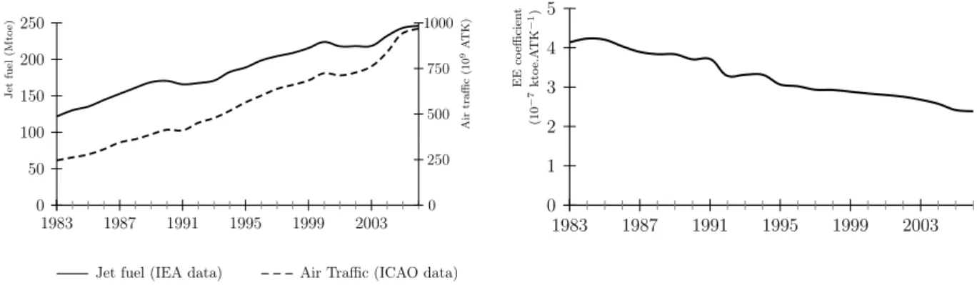
energy efficiency coefficients – i.e. for the aircraft fleet of a specific geographical zone, taken as whole – and (ii) their corresponding energy efficiency gains. Both are obtained based on empirical data obtained from the IEA and the ICAO. Energy efficiency coefficients and their evolution rules (i.e. energy efficiency gains) until 2025 are obtained by directly comparing the evolution of jet fuel consumption (taken from IEA data) and air traffic (taken from ICAO data). Figure 3 illustrates this approach21.
0 50 100 150 200 250 1983 1987 1991 1995 1999 2003 0 250 500 750 1000 Jet fu el (M to e) A ir tr a ffi c (1 0 9 A T K ) 0 1 2 3 4 5 1983 1987 1991 1995 1999 2003 E E co effi ci en t (1 0 − 7 k to e. A T K − 1)
Jet fuel (IEA data) Air Traffic (ICAO data)
Figure 3: Jet fuel consumption (Million Tonnes of Oil Equivalent (Mtoe)), Air traffic (ATK, billions) and Energy Efficiency (EE) coefficients at the world level. Illustration of the approach used to compute EE coefficients and their yearly growth rates (i.e. energy efficiency gains) for the aviation sector.
Source: Authors, from ICAO and IEA data.
These results are commented in Chèze et al. (2012) and summarized in Chèze et al. (2011). We thus only present here the main conclusions, i.e. the three “Traffic efficiency improvements” scenarios. These scenarios are defined according to the following results on [air traffic] energy [efficiency] gains: (i) some regions are more energy efficient than others, and (ii) regions do not encounter the same energy gains. By combining the current energy
21
In Figure 3 (left panel), the dotted black line represents air traffic (expressed in ATK) and the solid black line represents jet fuel consumption (expressed in Mtoe) for a given region. As explained in Chèze et al. (2011, 2012), energy efficiency coefficients for each year may be obtained by computing Mtoe/ATK (right panel), where ATK means “Available Tonne kilometre”. Thus defined, Energy Efficiency (EE) coefficients correspond to the quantity of jet fuel required to power the transportation of one tonne over one kilometre. For a given regional aircraft fleet, EEt+1 < EEtmeans that quantities of jet fuel required to power the transportation of
one tonne over one kilometre have decreased. Thus, a negative growth rate of EE coefficients, as it is expected, indicates the realization of energy efficiency improvements in air traffic for the region under consideration. As it may be deduced from the illustrative Figure 3, EE coefficients negative growth rates arise when, in a given year, jet fuel consumption growth rates are slower than air traffic ones.
efficiency coefficients of a given region with assumptions on their evolution during the next decade, we obtain the following three “Traffic efficiency improvements” scenarios based on the “energy efficiency gains” scenarios:
• “Heterogeneous energy gains’: this scenario aims at reflecting the heterogeneity of energy gains observed among regions during the past. For each regions, this scenario defines future (i) energy gains and (ii) load factor improvements, i.e. future “[air] traffic effi-ciency improvements”. Globally, this scenario defines the future energy gains of a given region as corresponding to the energy gains recorded during the period 1996-200822(see Table 1)23.
EE coefficients yearly growth rate by regions
Central and Europe Latin Russia Africa The Middle Asian countries China World
North America America and CIS East and Oceania
-3.18% -1.20% -1.63% -5.79% -4.2% -4.2% -1.54% -1.65% -2.22% *
Notes:
- Negative growth rate of EE coefficients indicates the realization of energy efficiency improvements in air traffic for the region under consideration.
* This figure corresponds to the world level energy gains (per year until 2025) resulting from regional energy gains hypothesis as defined in the ‘Heterogeneous energy gains’ traffic efficiency improvements scenario.
Table 1: EE coefficients yearly mean growth rates – by region and worldwide – retained for the “Heterogeneous energy gains” scenario of traffic efficiency improvements hypothesis (sc. A, see Figure 4) for the period 2008–2025.
Source: Authors (Chèze et al., 2012), from ICAO and IEA data.
• “Low energy gains’: “Heterogeneous energy gains” hypothesis are decreased by 10%. • “High energy gains’: “Heterogeneous energy gains” hypothesis are increased by 10%. 2.2.2 The nine “Air traffic CO2 emissions projection” scenarios
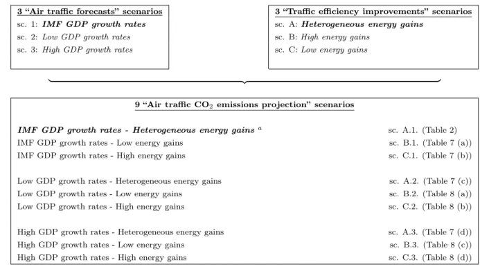
Sections 2.1 and 2.2.1 have respectively presented (i) three “air traffic forecasts” scenarios and (ii) three “energy efficiency gains” (i.e. energy efficiency improvements) scenarios. By
22
To have more realistic assumptions, some exceptions are made for some regions. See Chèze et al. (2010, 2011) for more details.
23
Regarding the evolution of each region’s weight load factor (WLF) until 2025, it is assumed that, when positive, the WLF yearly mean growth rate of the period 1983-2006 is applied until the region’s WLF reaches the 75% value. Otherwise, the WLF yearly mean growth rate of the period 1996-2006 is applied until it reaches the 75% value. See Chèze et al. (2010) for more details.
combining these scenarios, we obtain nine “Air traffic CO2 emissions projection” scenarios, as summarized in Figure 4.
3 “Air traffic forecasts” scenarios 3 “Traffic efficiency improvements” scenarios
sc. 1: IMF GDP growth rates sc. A: Heterogeneous energy gains
sc. 2: Low GDP growth rates sc. B: High energy gains
sc. 3: High GDP growth rates sc. C: Low energy gains
| {z }
9 “Air traffic CO2 emissions projection” scenarios
IMF GDP growth rates - Heterogeneous energy gainsa
sc. A.1. (Table 2)
IMF GDP growth rates - Low energy gains sc. B.1. (Table 7 (a))
IMF GDP growth rates - High energy gains sc. C.1. (Table 7 (b))
Low GDP growth rates - Heterogeneous energy gains sc. A.2. (Table 7 (c))
Low GDP growth rates - Low energy gains sc. B.2. (Table 8 (a))
Low GDP growth rates - High energy gains sc. C.2. (Table 8 (b))
High GDP growth rates - Heterogeneous energy gains sc. A.3. (Table 7 (d))
High GDP growth rates - Low energy gains sc. B.3. (Table 8 (c))
High GDP growth rates - High energy gains sc. C.3. (Table 8 (d))
a The “IMF GDP growth rates” air traffic forecasts scenario combined with the “Heterogeneous energy gains”
traffic efficiency improvements scenario corresponds to the Benchmark scenario (sc. A.1.). This scenario is summarized in Table 2.
The term ‘Heterogeneous’ means that the scenario relies on the hypothesis of varying energy efficiency gains between regions (contrary to an homogenous case). See Section 2.2.1 for more details.
2.2.3 Projections of air traffic CO2 emissions: the Benchmark scenario
We turn now to the presentation of our results. The benchmark scenario relies on the hypothe-ses coming from the “IMF GDP growth rates” scenario of evolution of air traffic, and from the “Heterogeneous energy gains” scenario of evolution of energy efficiency (sc. A.1., see Figure 4). Table 2 contains the forecasts of CO2 emissions obtained with the benchmark scenario for different regions and the world. According to the benchmark scenario, the CO2 emissions coming from air transport should rise from 725 Mt in 2008 to nearly 1,000 Mt in 2025 at the world level, i.e. an increase by 38% (1.9% per year on average) in less than two decades. This increase is due to the growth of air traffic by 4.7% per year on average on the one hand, and to the hypothesis of increasing the energy efficiency of the aircraft fleet by 2.2% per year on the other hand. These projections of air traffic are globally in line with previous literature (Airbus, 2007; Boeing, 2009). The hypothesis concerning the evolution of energy efficiency (2.2% per year, i.e. an improvement of 32% between 2008 and 202524) is globally higher than the values found typically in the literature25. More importantly, the values picked in this scenario are above the objectives of the airline industry.
At the regional level, Table 2 shows that the growth potential of air traffic lies in Asia, with an increase comprised between 6.9% and 8.2% per year on average26. Hence, the CO
2 emissions coming from Asia and China should sharply increase by, respectively, 126% and 170% from 2008 to 2025. In North-America and Europe, the share of these regions in CO2 emissions coming from air transport should on the contrary decrease, going from 60% to less than 50%.
Our benchmark scenario therefore anticipates a strong growth of CO2 emissions coming from air transport, even if it relies on optimistic assumptions of energy efficiency improvement for the aircraft fleet. This evolution implies a deep transformation of the repartition of CO2 emissions between regions from 2008 to 2025. Indeed, North America and Europe would still remain the geographic zones predominantly emitting greenhouse gases, but the share of these
24
This percentage expressed in absolute value corresponds to -2.2%/year cumulated over seventeen years. As illustrated in Figure 3, the energy efficiency of region i at time t is expressed in terms of M toei,t
AT Ki,t. Thus, a
negative growth rate corresponds to a gain (and not a decrease) in energy efficiency.
25
Currently, the values typically found in the literature are comprised between 1.5%/year (Lee et al., 2004) and 2.2%/year (Airbus, 2007 and 2009). See Eyers et al. (2004) and Mayor and Tol (2010) for a literature review.
26
Regions RTK (109
) CO2(Mt) Average annual (Energy gains hypothesis) (average annual (region’s share) growth rate of
growth rate) CO2emissions
2008 2025 2008 2025 (2008-2025) North and Central 246.2 405.9 274.43 246.11 -0.6% America (-3.18%) (3.0%) 37.9% 24.6%
Europe 163.5 310.0 162.89 233.01 2,2%
(-1.20%) (3.9%) 22.5% 23.3%
Latin America 28.5 64.7 54.97 78.81 2,2%
(-1.63%) (5.0%) 7.6% 7.9%
Russia and CIS 9.6 21.1 28.51 18.95 -2.2%
(-5.79%) (4.9%) 3.9% 1.9%
Africa 9.9 30.0 24.38 32.42 1,7%
(-4.20%) (6.7%) 3.4% 3.2%
The Middle East 24.1 48.7 24.98 22.43 -0.3%
(-4.20%) (4.5%) 3.5% 2.2% Asian countries 98.6 296.4 106.09 239.62 5,2% and Oceania (-1.54%) (6.9%) 14.7% 24.0% China 56.9 215.0 47.64 128.68 6,1% (-1.65%) (8.2%) 6.6% 12.9% World 637.4 1391.8 723.88 1000.03 1,9% (-2.22%)* (4.7%) 100% 100% Notes:
- The first column presents 2008 and 2025 air traffic forecasts expressed in RTK (for more details, see Section 2.1). Figures into brackets represent yearly mean growth rate of air traffic forecasts between 2008 and 2025.
- The other two columns concern air traffic CO2projections.
The second column presents 2008 and 2025 CO2 emissions forecasts expressed in million tonnes (Mt). For each geographical
region, CO2emissions projections are computed from jet fuel forecasts by using a factor of 3.156. Jet fuel forecasts are computed
from air traffic ones according to assumptions made on traffic efficiency improvements (for more details, see Section 2.2.1). In the second column, figures expressed in % terms indicate the share of each region’s CO2 emissions in 2008 and 2025.
Finally, the third column indicates the % yearly mean growth rate of CO2emissions projections between 2008 and 2025.
* This figure corresponds to the world level energy gains (per year until 2025) resulting from regional energy gains hypothesis as defined in the ‘Heterogeneous energy gains’ traffic efficiency improvements scenario.
Table 2: Air traffic (expressed in billion RTK) and corresponding CO2 emissions (expressed in million tonnes (Mt)) projections for the years 2008 and 2025 – Benchmark scenario, i.e. sc. A.1. (see Figure 4). Forecasts are presented at the world level (last line) and for each geographical regions (other lines).
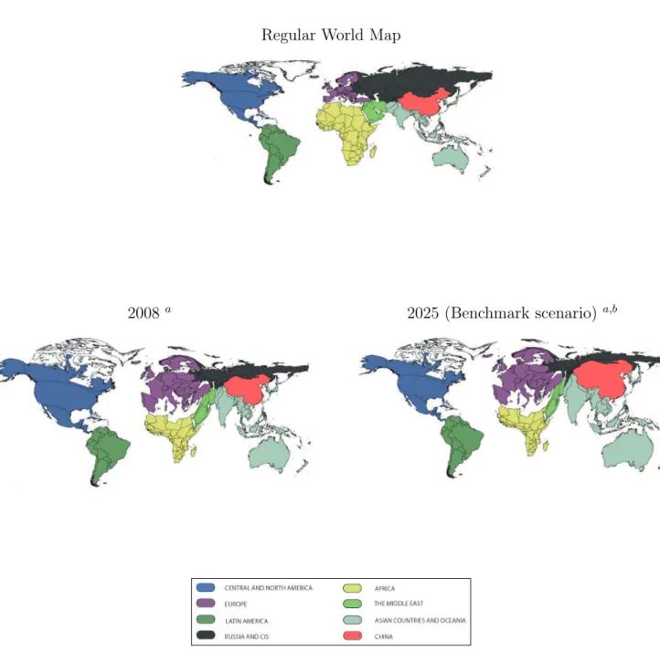
two regions would for the first time be inferior to 50%. Asia would represent almost a third of the total CO2 emissions coming from the air transport sector by 2025. Figure 5 illustrates these comments by proposing an alternative view of the share of each region’s CO2 emissions in 2008 and 2025. This expected change in the structure of repartition of emissions in the air transport sector highlights that it would be very difficult to decrease the level of global avia-tion emissions, at least in the medium term. Effectively, it is more costly (in terms of GDP points) to reduce GHG emissions in emerging countries (with high growth rates) compared to developed countries (Quinet, 2009).
Regular World Map
2008 a 2025 (Benchmark scenario)a,b
Notes:
a
These cartograms size the geographical zones according to their relative weight in world CO2 emissions
(expressed in Mt), offering an alternative view to a regular map of their projected evolution from 2008 to 2025. Maps generated using ScapeToad.
b
Projections realized according to the “IMF GDP growth rates” air traffic forecasts scenario combined with the “Heterogeneous energy gains” traffic efficiency improvements scenario, i.e. the “Benchmark ” Air traffic CO2 emissions projection scenario (sc. A.1., as synthesized in Figure 4).
Figure 5: An alternative view of the projected evolution of the share of each region’s CO2 emissions in 2008 and 2025.
2.2.4 Projections of air traffic CO2 emissions: sensitivity analysis
The sensitivity analysis of the benchmark scenario is concentrated around (i) the evolution of economic growth assumptions, and (ii) the assumptions regarding the energy efficiency improvements of the aircraft fleet. To do so, we define three scenarios for each type of hy-pothesis, which yields to nine different scenarios of CO2 emissions forecasts coming from air transport (see Figure 4). Forecasts of the eight alternative scenarios compared to the bench-mark scenario are shown in Tables 7 to 8 (see Appendix).
Figure 6 summarizes the results of four alternative scenarios, along with the benchmark scenario. Graph (a) shows the sensitivity of these results to the assumptions on energy efficiency improvements. CO2 emissions forecasts at the world level depend on decreases (Table 7.a and Figure 6, gray dashed curve) or increases (Table 7.b and Figure 6, black dashed curve) by 10% of the energy efficiency of the aircraft fleet compared to the benchmark scenario (Table 2 and Figure 6, bold curve). Graph (b) shows the sensitivity of these results to the assumptions on GDP forecasts. CO2 emissions forecasts at the world level depend on decreases (Table 7.c and Figure 6, gray dashed curve) or increases (Table 7.d and Figure 6, black dashed curve) by 10% of the level of expected economic activity compared to the benchmark scenario (Table 2 and Figure 6, bold curve).
500 600 700 800 900 1000 1100 2010 2013 2016 2019 2022 2025 C O2 emi ss io ns fro m ai r tra ns p ort (M t) 500 600 700 800 900 1000 1100 2010 2013 2016 2019 2022 2025 C O2 emi ss io ns fro m ai r tra ns p ort (M t)
IMF GDP growth rates + Low energy gains (sc. B.1.) IMF GDP growth rates + High energy gains (sc. C.1.) Benchmark scenario (sc. A.1.)
Heterogeneous energy gains + Low GDP growth rates (sc. A.2.) Heterogeneous energy gains + High GDP growth rates (sc. A.3.) Benchmark scenario (sc. A.1.)
(a) Sensitivity to the assumptions on energy effi-ciency improvements.
(b) Sensitivity to the assumptions on GDP fore-casts.
According to Figure 6.a, a decrease (an increase) by 10% of the assumptions on energy efficiency improvements compared to the benchmark scenario yields to an increase (a decrease) of CO2 emissions coming from air transport by 4.2% (4%) in 2025 (see Tables 2, 7.a and 7.b). According to Figure 6.b, a decrease (an increase) by 10% of the assumptions on the expected level of economic activity compared to the benchmark scenario yields to a decrease (an increase) of CO2 emissions coming from air transport by 8.8% (9.8%) in 2025 (see Tables 2, 7.c and 8.b).
Ceteris paribus, CO2 emissions coming from air transport therefore seem to be more sensitive to the variation of economic activity than to the variation of energy efficiency im-provements. Moreover, by comparing the forecasts of these nine scenarios, we observe that the CO2 emissions coming from air transport should rise between 22% (Table 8.b) and 57% (Table 8.c) at the world level.
None of the scenarios considered yields to a decrease, or even a stabilization, of the level of emissions by 2025. This result is obtained despite the introduction of strong hypotheses on energy efficiency gains in the air transport sector. Therefore, the improvement in energy efficiency alone does not appear to be sufficient to compensate for the increase in air traffic and its negative environmental consequences.
2.3
How much improvement in energy efficiency is needed to
stabi-lize the CO
2emissions coming from air transport?
Let us investigate here the hypothetical case where the increase in the energy efficiency of the aircraft fleet would stabilize (at the current levels of 700 Mt) the air transport CO2 emissions by 2025. The results of this scenario are shown in Table 3.
To stabilize CO2 emissions without constraining the demand for air transport, our results suggest that energy efficiency should be improved by 4% per year on average for the world aircraft fleet, i.e. an increase by 50% in seventeen years. This result implies that the hypoth-esis on energy efficiency improvements should be multiplied by two compared to our (already optimistic at 2.2% per year, see Table 2) benchmark scenario. A the time of writing, and given the current technological standards, such a high level of improvement seems unrealistic. Without limits on the demand for air transport, it appears therefore that CO2 emissions will increase significantly, unless major economic and/or exogenous shocks (such as the sub-prime crisis or the 9/11 terrorist attacks) occur during the period. Besides, we have shown earlier that CO2 emissions forecasts are more sensitive to changes in GDP growth forecasts compared
to energy efficiency improvements.
Regions RTK (109
) CO2(Mt) Average annual (Energy gains hypothesis) (average annual (region’s share) growth rate of
growth rate) CO2
2008 2025 2008 2025 (2008-2025) Central and North 246.2 405.9 258.45 139.17 -3.6% America (-6.04%) (3.0%) 37.4% 19.9%
Europe 163.5 310.0 159.34 189.10 1,1%
(-2.28%) (3.9%) 23.0% 27.1%
Latin America 28.5 64.7 53.34 59.24 0,7%
(-3.10%) (5.0%) 7.7% 8.5%
Russia and CIS 9.6 21.1 25.44 6.43 -7.6%
(-11.00%) (4.9%) 3.7% 0.9%
Africa 9.9 30.0 22.49 15.09 -2.3%
(-7.98%) (6.7%) 3.3% 2.2%
The Middle East 24.1 48.7 23.05 10.44 -4.3%
(-7.98%) (4.5%) 3.3% 1.5% Asian countries 98.6 296.4 1 103.13 183.04 3,7% and Oceania (-2.93%) (6.9%) 14.9% 26.2% China 56.9 215.0 46.22 96.38 4,5% (-3.14%) (8.2%) 6.7% 13.8% World 637.4 1391.8 691.45 698.87 0,1% (-4%)* (4.7%) 100% 100% Notes:
- The first column presents 2008 and 2025 air traffic forecasts expressed in RTK (for more details, see Section 2.1). Figures into brackets represent yearly mean growth rate of air traffic forecasts between 2008 and 2025.
- The other two columns concern air traffic CO2projections.
The second column presents 2008 and 2025 CO2 emissions forecasts expressed in million tonnes (Mt). For each geographical
region, CO2emissions projections are computed from jet fuel forecasts by using a factor of 3.156. Jet fuel forecasts are computed
from air traffic ones according to assumptions made on traffic efficiency improvements (for more details, see Section 2.2.1). In the second column, figures expressed in % terms indicate the share of each region’s CO2 emissions in 2008 and 2025.
Finally, the third column indicates the % yearly mean growth rate of CO2emissions projections between 2008 and 2025.
* This figure corresponds to the world level energy gains (per year until 2025) resulting from regional energy gains hypothesis.
Table 3: Air traffic (expressed in billion RTK) and CO2 emissions (expressed in million tonnes (Mt)) forecasts for the years 2008 and 2025. Forecasts are presented at the world level (last line) and for each geographical regions (other lines). Hypothetical case where the increase in the energy efficiency of the aircraft fleet would stabilize (at the current levels of 700 Mt) the air transport CO2 emissions by 2025.
3
Comparing our estimates with previous literature and
the SRES scenarios from the IPCC
This Section compares the results obtained in this article with previous literature. We compare first our CO2 emissions forecasts in the air transport sector with the estimates found in other
studies, before confronting them to the SRES scenarios by the IPCC (Nakicenovic and Swart, 2000; IPCC, 2007a, 2007b). Note that previous studies differ in terms of hypotheses, which makes difficult the direct comparison with our estimates. The comparison with the IPCC SRES scenarios is detailed in Section 3.2.
3.1
Comparison with other CO
2emissions forecasts from air
trans-port
Table 4 summarizes the growth rates of CO2 emissions coming from air transport found in previous studies. These results show that CO2 emissions could rise from 0.8% to 4% per year during the next decade. The main differences between these forecasts are due to the under-lying model assumptions (economic growth rate, energy efficiency improvement, etc.) and to various geographical scopes. Figure 7 shows how these CO2 emissions from air transport are forecast by a number of studies and for many scenarios27. Note that our forecasts are lower than many of other forecasts.
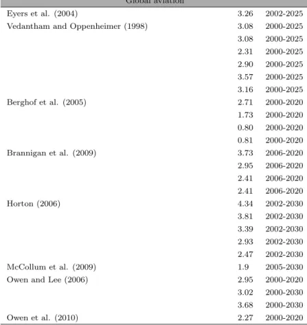
Assumptions regarding the GDP growth rate and energy efficiency improvements are the main determinants of the CO2 emissions forecasts. Besides, various scenarios co-exist. Mayor and Tol (2010) consider that CO2 emissions linked to international tourism are dependent on income rise, and that they must therefore increase (by a factor of twelve between 2005 and 2100 according to their baseline scenario). Macintosh and Wallace (2009) hypothesize that the increase in the demand for air transport cannot be compensated by energy efficiency improvements. Therefore, they estimate that CO2 emissions coming from air transport will increase by 110 % during 2005-2025 at the world level. Olsthoorn (2001) concludes that CO2 emissions coming from air transport will be in 2020 higher by 55% to 105% compared to base-line emissions in 2000. Vedantham and Oppenheimer (1998), Eyers et al. (2004), Berghof et al. (2005), Brannigan et al. (2009), Horton (2006), McCollum et al. (2009), Owen and Lee (2006) and Owen et al. (2010) also propose CO2 emissions forecasts coming from air transport. Depending on the period under consideration, the underlying assumptions and the scenario adopted, these studies show that the CO2emissions coming from air transport should rise at a yearly mean growth rate comprised between 0.81% (Berghof et al., 2005) and 4.34 % (Horton, 2006) during the next twenty years at the world level. According to Vedantham
27
Gudmundsson and Anger (2012) summarize the aviation CO2 emissions studies of the IPCC IS92 and
Special Report on Emissions Scenarios storylines, where GDP growth assumptions contribute to forecast global CO2emissions from the aviation sector.
Global aviation
Eyers et al. (2004) 3.26 2002-2025
Vedantham and Oppenheimer (1998) 3.08 2000-2025 3.08 2000-2025 2.31 2000-2025 2.90 2000-2025 3.57 2000-2025 3.16 2000-2025 Berghof et al. (2005) 2.71 2000-2020 1.73 2000-2020 0.80 2000-2020 0.81 2000-2020 Brannigan et al. (2009) 3.73 2006-2020 2.95 2006-2020 2.41 2006-2020 2.41 2006-2020 Horton (2006) 4.34 2002-2030 3.81 2002-2030 3.39 2002-2030 2.93 2002-2030 2.47 2002-2030 McCollum et al. (2009) 1.9 2005-2030
Owen and Lee (2006) 2.95 2000-2020
3.02 2000-2030 3.68 2000-2030
Owen et al. (2010) 2.27 2000-2020
Table 4: Annual growth rates of global aviation carbon dioxide emissions
and Oppenheimer (1998), the yearly mean growth rate of CO2 emissions in the air transport sector should be in the interval [2.31%;3.57%] (i.e. between 1,430 Mt and 1,943 Mt) until 2025. Eyers et al. (2004) estimate that the CO2 emissions coming from air transport will be multiplied by a factor of two between 2002 and 2025 to reach 1,029 Mt per year. Berghof et al. (2005) estimate that CO2 emissions should be multiplied by a factor comprised between 1.2 and 1.9 during 2000-2020 to reach 880 Mt-1,049 Mt. Horton (2006) estimates that CO2 emissions from air transport should be in the range of 970 Mt to 1,609 Mt (from a baseline of 489 Mt in 2002). Brannigan et al. (2009) estimate that CO2 emissions from air transport will increase by 2.41% to 3.73% per year during 2006-2020 (i.e. 879 Mt to 1,048 Mt CO2 per year in 2020). Owen and Lee (2006) estimate that CO2 emissions from air transport will be comprised between 1,172 Mt and 1,420 Mt by 2030, i.e. an increase by 3.02% to 3.68% per year during 2000-2030. Owen et al. (2010) estimate the CO2 emissions should be multiplied by a factor of 1.5 during 2000-2020, and by 2-3.6 during 2000-2050. Finally, McCollum et al. (2009) anticipate that CO2 emissions from air transport will be multiplied by a factor of two during 2005-2030.
0 200 400 600 800 1000 1200 1400 1600 1800 2000 1995 2000 2005 2010 2015 2020 2025 2030 u u u b c b c b c b c u t u t u t u t r r r r l l l l × × × × × b b b b b b Eyers et al. (2004)
Vedantham and Oppenheimer (1998) Berghof et al. (2005)
Brannigan et al. (2009)
Horton (2006) Owen and Lee (2006) Owen et al. (2010)
Benchmark scenario (this study)
C O2 em is si on s (M t p .y .) Notes:
- Differences between CO2data on past and current aviation emissions tend to come from differences in fuel
sold data sources and assumptions (Brannigan et al., 2009). - Only low and high estimates are provided.
Figure 7: Comparison of results from global aviation emission studies, 1995-2030, Mt CO2. The forecasts of CO2 emissions from air transport based on our benchmark scenario are in the lower range compared to previous estimates. Namely, we have more optimistic assump-tions regarding the improvements in energy efficiency compared to other studies. Besides, our forecasts take into account the global economic downturn since 2007-2008, which had an adverse impact on air traffic and therefore CO2 emissions from 2008 to 2010 (see Figures 2 and 6), whereas previous studies did not.
The next Section compares our estimates with the IPCC SRES scenarios (Nakicenovic and Swart (2000)).
3.2
Comparisons with the SRES scenarios from Nakicenovic and
Swart (2000)
The overwhelming conclusion among previous studies is that CO2 emissions coming from air transport are strictly anticipated to increase in the near future. Even with optimistic as-sumptions on energy efficiency improvements, our benchmark scenario concludes that CO2 emissions will increase by 40% in 2025. These results suggest that the air transport sector is not currently compatible with sustainable development, at least in the mid-term. To analyze more in depth this assertion, we propose in the next Sections to compare our projections of air transport CO2 emissions with the SRES scenarios from Nakicenovic and Swart (2000). By doing so, we will be able to check if our projections are effectively compatible, or not, with the objective of limiting global warming to 2◦C (IPCC, 2007a, 2007b).
Before presenting our comparison, we first detail briefly below the SRES scenarios. 3.2.1 SRES scenarios from Nakicenovic and Swart (2000)
To limit global warming to 2◦C compared to pre-industrial levels, Nakicenovic and Swart (2000) have elaborated several scenarios which simulate the evolution of greenhouse gases linked to human activity until 2100: the SRES scenarios, for “Special Report on Emission Scenarios”. These scenarios rely on several assumptions regarding world economic growth and population growth, the growth of developing countries, environmental quality and tech-nology diffusion (IPCC, 2007a, 2007b).
As shown in Figure 8, the maximum concentration of greenhouse gases in the atmosphere should not exceed 450ppm in order to limit the increase in temperatures to +2◦C. This target implies a stabilization of world emissions by 2020-2025, and a reduction by a factor of two by 2050 (in the Type I scenario). Table 5 (taken from Quinet, 2009) proposes another view of these results. In the “pessimistic” IPCC scenarios (types V and VI), global warming may be as high as +6.1◦C in 2100 compared to 1900.
Figure 8: Stabilization and equilibrium global mean temperatures.Source: IPCC (2007a). Class Anthropogenic addition to radiative forcing at stabilization (W/m2 ) Stabilization level for CO2 only, con-sistent with multi-gas level (ppm CO2) Multi-gas concentra-tion level (ppm CO2 -eq) Global mean temperature C increase above pre-industrial at equilibrium, using best esti-mate of cliesti-mate sensitivity Peaking year for CO2 emis-sions Change in global emis-sions in 2050 (% of 2000 emissions) Number of assessed scenario I 2.5 - 3.0 350 - 400 445 - 490 2.0 - 2.4 2000 - 2015 -85 to -50 6 II 3.0 - 3.5 400 - 440 490 - 535 2.4 - 2.8 2000 - 2020 -60 to -30 18 III 3.5 - 4.0 440 - 485 535 - 590 2.8 - 3.2 2010 - 2030 -30 to +5 21 IV 4.0 - 5.0 485 - 570 590 - 710 3.2 - 4.0 2020 - 2060 +10 to +60 118 V 5.0 - 6.0 570 - 660 710 - 855 4.0 - 4.9 2050 - 2080 +25 to +85 9 VI 6.0 - 7.5 660 - 790 855 - 1130 4.9 - 6.1 2060 - 2090 +90 to +140 5 TOTAL 177
Table 5: Properties of emissions pathways for alternative CO2 and CO2-eq stabilization tar-gets.
Source: Quinet (2009), from IPCC (2007a).
3.2.2 Comparisons between our air traffic CO2 emissions projections scenarios and the IPCC ones
Table 6 compares our CO2 emissions forecasts coming from air transport (lines, in gray) with worldwide CO2 emissions coming from the IPCC scenarios of type I, III, and IV28 (columns, in blue) until 2025.
Let us first detail the comparison of our benchmark scenario with the three SRES scenar-ios contained in Table 6. This Table recalls the total of world CO2 emissions, expressed in
28
The IPCC scenarios of type V and VI have been deliberately dismissed, as they would yield to unsustain-ably high levels of climate change.
Mt, in 2008 and 2025 coming from the SRES scenarios (columns ‘Total’, in blue). Thus, for global warming to stay within the limit of 2-2.4◦C in 2100 (IPCC scenario of type I), CO
2 emissions should be strictly inferior to 29,000 Mt in 2025 (Table 6, 1st column, 2nd row). World CO2 emissions should therefore be stable between 2008 and 2025 (Table 6, 1st column, 3rd row). For global warming to stay within the limit of 2.8-3.2◦C in 2100 (IPCC scenario of type III), CO2 emissions should be strictly inferior to 34,500 Mt in 2025 (Table 6, 4th column, 2nd row). World CO2 emissions should therefore increase by 19% between 2008 and 2025 (Table 6, 4th column, 3rd row). For global warming to stay within the limit of 3.2-4◦C in 2100 (IPCC scenario of type III), CO2 emissions should be strictly inferior to 39,500 Mt in 2025 (Table 6, 7th column, 2nd row). World CO2 emissions should therefore increase by 36% between 2008 and 2025 (Table 6, 7th column, 3rd row). Then, we recall our projections of CO2 emissions in the air transport sector coming from our ten scenarios (columns ‘Aviation’, in gray). According to our benchmark scenario, CO2 emissions from air transport should rise from 724 Mt in 2008 (Table 6, 2nd column, 1st row) to 1,000 Mt in 2025 (Table 6, 2nd column, 2nd row), i.e. an increase by 38% (Table 6, 2nd column, 3rd row). The comparison between our projections and the SRES scenarios is performed by computing the share of CO2 emissions from the air transport sector in the total of world emissions in 2008 and 2025 (Table 6, column ‘Share’). For instance, the share of CO2 emissions coming from air transport in total CO2emissions at the world level is equal to 2.5% in 2008 (Table 6, 3rd column, 1st row). Table 6 indicates that, to reach the objective of limiting global warming to +2◦C in 2100 as in the Type I SRES scenarios, CO2 emissions from aviation in our benchmark scenario should represent 3.4% of world emissions in 2025 (Table 6, 3rd column, 2nd row). This would represent an increase of the share of emissions from aviation in total emissions by 38% be-tween 2008 and 2025 (Table 6, 3rd column, 3rd row). This figure is represented in red to show an increase. More importantly, it reveals that this growth of emissions from aviation is not compatible with the objective of 450 ppm (Type I SRES scenarios) recommended by the IPCC (2007a, 2007b). This growth of emissions from aviation is not compatible either with the objective of limiting global warming to +3.2◦C in 2100 as in the Type III SRES scenarios. Indeed, the share of emissions from aviation should go from 2.5% in 2008 (Table 6, 6th column, 1st row) to 2.9% in 2025 (Table 6, 6th column, 2nd row), i.e. an increase by 16% (Table 6, 6th column, 3rd row). Actually, the forecasts from our benchmark scenario are only compatible with an increase of temperatures between +3.2 and +4◦C if world emis-sions remain on the same growth rate. The share of air transport emisemis-sions would effectively remain constant between 2008 and 2025 with a percentage of variation of 1% only (Table 6,
9th column, 3rd row) as shown in green.
Finally, according to Table 6, none of our nine scenarios of CO2 emissions from aviation is compatible with the objective of limiting global warming to +3.2◦C (Types I to III SRES scenarios)29. Only the scenario presented in Table 3 is compatible with the objective of 450 ppme. Again, this result is conform to our expectations, since this scenario has been explicitly created to meet the objective by stabilizing CO2 emissions from aviation between 2008 and 2025 (see Section 2.3).
29
IPCC scenario of type I IPCC scenario of type III IPCC scenario of type IV
(445-490 ppm. i.e. 2.0-2.4oC) (535-590 ppm. i.e. 2.8-3.2oC) (590-710 ppm. i.e. 3.2-4.0oC)
Total Aviation Share Total Aviation Share Total Aviation Share
(Mt) (Mt) (%) (Mt) (Mt) (%) (Mt) (Mt) (%)
Benchmark scenario A.1. 2008 29000 724 2.5% 29000 724 2.5% 29000 724 2.5%
(table 2∗) 2025 29000 1000 3.4% 34500 1000 2.9% 39500 1000 2.5% Variation 0% 38% 38% 19% 38% 16% 36% 38% 1% scenario B.1. 2008 29000 728 2.5% 29000 728 2.5% 29000 728 2.5% of table 7.a∗ 2025 29000 1042 3.6% 34500 1042 3.0% 39500 1042 2.6% Variation 0% 43% 43% 19% 43% 20% 36% 43% 5% scenario C.1. 2008 29000 720 2.5% 29000 720 2.5% 29000 720 2.5% of table 7.b∗ 2025 29000 960 3.3% 34500 960 2.8% 39500 960 2.4% Variation 0% 33% 33% 19% 33% 12% 36% 33% -2% scenario A.2. 2008 29000 723 2.5% 29000 723 2.5% 29000 723 2.5% of table 7.c∗ 2025 29000 912 3.1% 34500 912 2.6% 39500 912 2.3% Variation 0% 26% 26% 19% 26% 6% 36% 26% -7% scenario A.3. 2008 29000 725 2.5% 29000 725 2.5% 29000 725 2.5% of table 7.d∗ 2025 29000 1099 3.8% 34500 1099 3.2% 39500 1099 2.8% Variation 0% 52% 52% 19% 52% 27% 36% 52% 11% scenario B.2. 2008 29000 727 2.5% 29000 727 2.5% 29000 727 2.5% of table 8.a∗ 2025 29000 951 3.3% 34500 951 2.8% 39500 951 2.4% Variation 0% 31% 31% 19% 31% 10% 36% 31% -4% scenario C.2. 2008 29000 719 2.5% 29000 719 2.5% 29000 719 2.5% of table 8.b∗ 2025 29000 875 3.0% 34500 875 2.5% 39500 875 2.2% Variation 0% 22% 22% 19% 22% 2% 36% 22% -11% scenario B.3. 2008 29000 729 2.5% 29000 729 2.5% 29000 729 2.5% of table 8.c∗ 2025 29000 1145 3.9% 34500 1145 3.3% 39500 1145 2.9% Variation 0% 57% 57% 19% 57% 32% 36% 57% 15% scenario C.3. 2008 29000 721 2.5% 29000 721 2.5% 29000 721 2.5% of table 8.d∗ 2025 29000 1055 3.6% 34500 1055 3.1% 39500 1055 2.7% Variation 0% 46% 46% 19% 46% 23% 36% 46% 7% scenario 2008 29000 691 2.4% 29000 691 2.4% 29000 691 2.4% of table 3∗ 2025 29000 699 2.4% 34500 699 2.0% 39500 699 1.8% Variation 0% 1% 1% 19% 1% -15% 36% 1% -26% Notes:
- “Total” corresponds to global CO2 emissions projections for 2008 and 2025 (expressed in Mt). These projections are provided by
Nakicenovic and Swart (2000) – scenarios of type I, III and IV, as specified in columns.
- “Aviation” corresponds to our aviation CO2emissions projections for 2008 and 2025 (expressed in Mt) for a given scenario specified in
lines.
- “Share” corresponds to aviation’s share of global CO2emissions in 2008 and 2025 (expressed in %).
- A red (green) value means that this share will increase (decrease) between 2008 and 2025. Hence, a red (green) value means that scenario is not compatible (compatible) with the given IPCC scenario (type I, III or IV).
* scenarios of Tables 2, 7 and 8 are presented in Figure 4. Scenario of table 3 is a hypothetical case where the increase in the energy efficiency of the aircraft fleet would stabilize the CO2emissions coming from air transport by 2025 (see Section 2.3).
Table 6: Comparison of the study’s CO2 forecasts with those provided by IPCC (scenarios of type I, III and IV).
4
Conclusion
CO2 emissions have grown substantially in the aviation sector over the last decades. Air transport is the world’s fastest growing source of greenhouse gases. Aviation contributes to about 8% of fuel consumption and between 2.5% and 3% of anthropogenic CO2 emissions (IEA, 2009a, 2009b, 2009c). At present, aviation cannot be considered as a major contributor to climate change. Nevertheless, its high growth rate attracts the attention of policy-makers. Addressing GHG emissions from aviation is challenging. Two types of mitigations options are distinguished: (i) technological and operational possibilities, and (ii) policy options (market based options such as EU-ETS or regulatory regimes). As it can be expected, these latter op-tions face fierce opposition by most stakeholders in the aeronautical industry. Nevertheless, it seems that anticipated technological progress would not be sufficient to completely annihilate the negative impact of aviation on the rise of CO2 emissions in the mid-term.
This paper contains forecasting results of world and regional aviation CO2 emissions to the mid-term (2025). To do so, it relies heavily on the econometric results and traffic effi-ciency improvement assumptions developed by Chèze et al. (2010, 2012) and summarized in Chèze et al. (2011). Following an econometric analysis of the relationship between air traffic and its main drivers, air traffic forecasts are converted into quantities of jet fuel by using a “macro level ” methodology, which allows obtaining energy efficiency coefficients without prior assumptions on the composition of the aircraft fleet. Chèze et al. (2010, 2011, 2012) only proposed jet fuel demand forecasts. This article goes one step further by presenting original air traffic C02 emissions deduced from the latter forecasts. By applying a specific energy factor30 to the quantity of jet fuel used, it is effectively readily possible to deduce the CO
2 emissions coming from the air transport sector. The projections of aviation CO2 emissions are provided for eight regions and at the world level (the sum of the eight regions). Nine scenarios of air traffic CO2 emissions projections are proposed. Depending on the scenario under consideration, the CO2 emissions coming from air traffic are projected to increase, at the world level, with yearly mean growth rates comprised between 1.2% (sc. C.2.) and 2.7% (sc. B.3.) from 2008 to 2025. Our Benchmark scenario (sc. A.1.) anticipates an increase of air traffic CO2 emissions of about 2% per year at the world level (i.e. about 38% in less than two decades), from 725 Mt of CO2 in 2008 to nearly 1,000 Mt in 2025, and ranging from -2.2% (Russia and CIS) to +6.1% (China) at the regional level.
30