Applying the Damage Rating Index for the spatial damage assessment in concrete specimens affected by alkali-silica reaction (ASR)

(1)

© Mathieu Champagne, 2020

Applying the Damage Rating Index for the spatial

damage assessment in concrete specimens affected by

alkali-silica reaction (ASR)

Mémoire

Mathieu Champagne

Maîtrise interuniversitaire en sciences de la Terre - avec mémoire

Maître ès sciences (M. Sc.)

(2)

Applying the Damage Rating Index for the spatial

damage assessment in concrete specimens affected by

alkali-silica reaction (ASR)

Mémoire

Mathieu Champagne

Sous la direction de :

Benoît Fournier, Directeur de recherche

Josée Duchesne, Codirectrice de recherche

(3)

iii

RÉSUMÉ

Ce mémoire de maîtrise présente les résultats de l’évaluation de l’endommagement d’une série de 35 éprouvettes de béton préalablement testés pour la réaction alcalis-silice (RAS) lors d’essais sur prismes de béton effectués dans le cadre du projet norvégien COIN. Ces prismes, confectionnés avec une variété de granulats réactifs et de matériaux cimentaires, ont été testés dans différentes conditions de laboratoire conformément à plusieurs normes d’essais utilisés en Amérique du Nord et en Europe.

Pour évaluer l’endommagement du béton, une méthode pétrographique de quantification de l’endommagement du béton a été utilisée, soit le Damage Rating Index (DRI). Lors de cet essai, un pétrographe comptabilise les indices d’endommagement à l’aide d’un stéréomicroscope (grossissement 15x) sur une plaque de béton polie, afin d’en identifier le nombre DRI. Cet essai est de plus en plus utilisé en Amérique du Nord; cependant, aucune procédure d’essai normalisée n’est encore disponible. Les objectifs de cette étude étaient 1), d’évaluer la répétabilité attribuable au même opérateur, 2), d’évaluer l’applicabilité du DRI à l’analyse spatiale de l’endommagement d’un même spécimen, 3), de valider si la méthode est efficace pour des bétons incorporant des ajouts cimentaires et 4), de confirmer si des indices pétrographiques attribuables à la RAS peuvent être observés à l’échelle du DRI sur des spécimens ayant atteint une expansion près de la limite de 0.040% ou moins.

La variabilié attribuable au même opérateur a été déterminée par ANOVA à l’aide d’un logiciel de statistique permettant d’analyser la variance dite «ponctuelle» à l’échelle d’un cm2_{. Les résultats ainsi obtenus démontre} que l’expérience de l’opérateur influence grandement la variabilité des résultats de l’essai, alors qu’une certaine expérience est requise pour obtenir une constance raisonable dans la réalisation de l’essai. Cela dit, une certaine variabilité demeure toujours présente, puisqu’un coefficient de variation ponctuel très élevé allant de 61.0 à 120.4% a été obtenu pour un opérateur expérimenté. Cette variabilité est directement reliée à l’endommagement du spécimen, i.e. pour un endommagement plus élevé, une variabilité (relative) plus faible est obtenue. En utilisant la théorie de l’échantillonage, une équation permettant d’évaluer la marge d’erreur (seuil de confiance de 95%) correspondant à l’incertitude intrumentale sur un nombre DRI obtenu par l’opérateur de cette étude sur un certain nombre de cm2_{a été obtenue. Bien que les coefficients de variation ponctuels} obtenus soient très élevés, l’incertitude d’un même opérateur à l’échelle d’une surface suffisamment grande (± 200 cm2_{) est de ≈11% (dépendant du niveau d’endommagement), ce qui est comparable à l’incertitude liée la} répétabilité (intra-laboratoire) mesurée pour plusieurs autres essais fréquemment utilisés tels que l’ASTM C457 (≈16%) ou l’ancienne RILEM AAR-3 (≈16-23%).

(4)

iv

Trois méthodes d’analyse spatiale de l’endommagement à partir du DRI ont été développées lors de cette étude, soit 1), l’évaluation du profil d’endommagement du béton par l’entremise de groupe de lignes (i.e. peau vs cœur selon l’axe longitudinal de l’éprouvette) ; 2), l’évaluation du profil d’endommagement du béton par l’entremise de zones d’égale dimension (e.g. 50 cm2_{) situées d’une extrémité à l’autre de l’éprouvette (sommet vers la} base) ; 3), une carte d’intensité de l’endommagement (DRI damage map) permettant une appréciation qualitative/visuelle de la variabilité de l’endommagement sur la surface entière de l’éprouvette. Les résultats obtenus démontrent que le DRI est assez sensible pour permettre l’analyse spatiale de l’endommagement pour un même spécimen si les variations d’endommagement locales sont présentes sur une surface suffisamment grande, c’est-à-dire ± 50 cm2_{. Cependant, le DRI damage map est considéré comme l’outil le moins fiable.} L’analyse spatiale de l’endommagement des prismes de béton suggère que certains mélanges cimentaires ou certaines conditions de laboratoire (e.g. lessivage des alcalis ou enveloppement des éprouvettes dans un tissu préalablement trempé dans une solution alcaline) peuvent générer différents patrons de fissuration à l’intérieur du prisme.

L’examen visuel par la méthode du DRI de prismes de béton manufacturés à partir de mélanges cimentaires différents (avec et sans ajouts cimentaires) ayant une expansion similaire a démontré qu’un niveau d’endommagement non négligeable peut parfois être observé dans des bétons incorporant des ajouts cimentaires mais relativement peu affectées par la RAS. Ces valeurs de DRI plus élevées sont entièrement causées par la présence de fines fissures dans le pâte de ciment. Il est suggéré que ces fissures résultent d’un autre mécanisme d’endommagement, tel que le retrait, et/ou que l’augmentation du contraste de couleur entre la pâte de ciment et ces fissures permet à l’opérateur de plus facilement les distinguer. Ce type de fissures a en effet été identifié principalement pour des bétons incorporant du laitier de hauts-fourneaux alors qu’elles ne furent pas observées pour les bétons fabriqués avec des cendres volantes.

L’examen pétrographique des prismes ayant subi une expansion entre 0.022 et 0.041% a démontré que plusieurs indices pétrographiques reliés à la RAS peuvent être observés à l’aide d’un stéréomicroscope à l’échelle du DRI (grossissement de 15x), et ce même à ce niveau d’expansion. De plus, certains indices d’endommagement attribuables à la RAS, tels que les fissures ouvertes dans les particules de granulat avec produits de réaction et les fissures dans la pâte de ciment avec produits de réaction, ont pu être observés à quelques reprises sur ces bétons faiblement endommagés. Cela mène à la conclusion que la RAS peut bel et bien être diagnostiquée lors de l’examen visuel d’une plaque de béton polie à l’échelle du DRI, et ce à une expansion aussi faible que 0.022%.

(5)

v

ABSTRACT

This MSc dissertation provides the results of quantitative damage assessments, using the Damage Rating Index (DRI) method and petrographic examination, of 35 concrete prisms that were manufactured with different aggregates and binders as well as being exposed to different testing conditions through the Norwegian COIN project. Visual examination of the test prisms was conducted with a stereomicroscope at a ≈15x magnification along with damage assessment through DRI. The objectives of the study were 1) to appraise the single operator variability of the DRI method, 2) appraise the “sensivity” of the method to apply damage spatial analysis within the same specimen, 3) validate whether the method is suited for the damage assessment in concrete incorporating SCMs and 4) confirm whether petrographic features of ASR can be identified at the DRI scale on specimens with an expansion close to the limit of 0.040% or lower.

Upon replicate DRI determinations on eight specimens, the single operator variability was determined for each square (cm2_{) within the test specimens by ANOVA. The results obtained highlighted that the experience of the} operator significantly influences the single operator variability and that a certain experience is required before achieving a reasonable consistency. The single operator variability determined at the scale of each square is considerably high with coefficients of variation ranging between 61.0 and 120.4%, depending on the magnitude of the DRI number of the specimen. The latter is directly influenced by the damage level of the specimen, i.e. the more damage - the lower the variability (from a relative point of view). By applying the sampling theory to the single operator variability found in this study, a margin of error related to the instrumental measurement

uncertainty was determined. It was found that the instrumental measurement uncertainty of the method (i.e. the

repeatability of the measuring instrument) for an experienced operator is equal to ≈11% (depending on the damage degree) when analysing approximately 200 cm2_._{The latter can be compared to other test methods} frequently used in laboratories like the former AAR-3 (≈16-23%) or the ASTM C457 (≈16%).

Three DRI spatial analysis tools were developed for this study, i.e. 1) the DRI damage mapping, 2) the analysis of grouped lines and 3) the damage profile. In summary, the DRI damage mapping consists in analysing the DRI number of each square separately and classifying them with a color code depending on the damage degree, hence qualitatively/visually identify damage contrast. The analysis of grouped lines consists in separating the specimen in grouped lines of equal distance (laterally) from the prism’s surface and assessing individually their respective DRI values within the specimen. The damage profile consists in separating the prism in zone of equal areas (4 or 9, depending on the prism size) from the top to the bottom and assess their respective DRI number. According to the results obtained in this study, the DRI method is “sensitive” enough for damage spatial analysis if local damage variations are present within an area large enough, i.e. ± 50 cm2_{, although the DRI damage} mapping is the less reliable of the above tools. Otherwise, the method’s single-operator precision (i.e.

(6)

vi

repeatability) is not high enough to provide a relatively good indication of the extent of damage variations at such small scale. Overall, the damage assessed within prisms suggest that some binder types or exposure conditions (e.g. alkali leaching or alkali wrapping) may induce certain internal damage variations.

Comparing the damage degree of prisms with equal expansion but different binder types (with and without SCMs) revealed a somewhat higher degree of damage assessed through the DRI method for some SCM-bearing specimens. In this study, the use of fly ash was found to have no effect on DRI number, whereas an increase in DRI number was found for specimens of similar expansion incorporating slag. This damage increment is largely due to an increase of counted cracks in the cement paste, which is believed to be either caused by another damage mechanism (such as shrinkage) or the higher contrast between the whitish cracks and the darker cement paste making them easier to be noticed by the operator.

Even for specimens with an expansion between 0.022 to 0.041%, several ASR petrographic features like voids of the cement paste filled/lined with secondary reaction products or reaction rims (depending on the aggregate type) can be noticed when conducting the DRI (with a stereomicroscope at ≈ 15x magnification). Other ASR damage features like opened cracks in the aggregate particles with reaction products or cracks in the cement paste with reaction products were also noticed in those specimens, although rare. This leads to the conclusion that ASR can be diagnosed visually when performing DRI determination on concrete specimens with an expansion as low as 0.022%.

(7)

vii

LIST OF FIGURES

Figure 1 : World map showing countries with known cases of deleterious AAR (black color), but

“incomplete” because it is in constant evolution, from Broekmans (2012). _______________________ 2 Figure 2 : Cracking pattern in concrete affected by ASR originating (a) from the fine aggregate fraction and

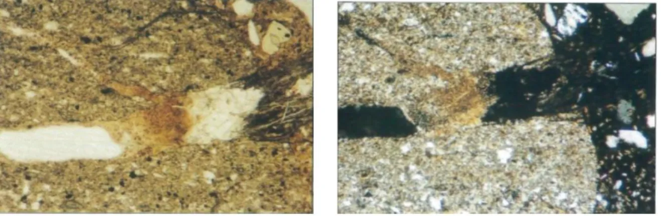
(b) from the coarse aggregate fraction, from BCA (1992). ____________________________________ 7 Figure 3 : Petrographic features of ASR observed at different scales: (A) Concrete under a stereomicroscope

(the line is ≈ 1cm), from Fournier et al. (2015b). (B) Thin section under an optical microscope with plane polarized light, from Poole & Sims (2016). (C, D) Concrete under a SEM equipped with an

energy-dispersive X-ray analyser, from Bérubé & Fournier (1986). _____________________________ 8 Figure 4 :Vein in concrete prism with locations L1 inside the aggregate particle (crystalline ASR product), L2

inside the aggregate particle but in contact with the cement paste (amorphous ASR product) and L3 inside the cement paste (amorphous ASR product), from Leemann (2017). _____________________ 11 Figure 5 : The distribution of the chemical composition of the ASR gels in the literature (Stanton, 1942;

McConnel et al., 1947; Hester & Smith, 1958; Idorn, 1961; Buck & Mather, 1969; Poole, 1975; Gutteridge & Hobbs, 1980; Oberholster, 1983; Visvesvaraya et al., 1986; Šachlováet al., 2010) (the x axes of (a) to (e) and (f) are atomic ratios and weight percent losses assumed to be chemically

absorbed water and OH-_{groups, respectively), from Gholizadeh Vayghan & Rajabipour (2017). _____ 12} Figure 6 : Atomic Ca-to-Si ratio against atomic Ca–to-(Na + K) ratio in ASR products within the aggregate

particle and in the cement paste, compared with C–S–H formed by the hydration of ordinary Portland cement, as analysed in a concrete produced with reactive volcanic rock, from Katayama (2012b). ___ 15 Figure 7 : Examples of cracking pattern observed in ASR affected aggregate particles of the Quebec

Province (Canada): (A) Peripheral cracking in reactive granitic aggregates. (B) Internal attack of the quartzitic cement in a siliceous sandstone. (C) Internal cracking through the formation of alkali-silica gel in siliceous limestones. Adapted from Bérard & Roux (1986). _____________________________ 16 Figure 8 : Schematic representation of the micro-level mechanism of ASR-induced cracking of concrete (R+

denotes an alkali ion: K+_{and Na}+_{), from Ichikawa & Miura (2007). ____________________________ 17} Figure 9 : A. Cross section of an ASR affected andesite particle (top) and its element mapping for calcium

(bottom), from Ichikawa & Miura (2007). ________________________________________________ 19 Figure 10 : Thin section showing a crack (left) which is empty apart from an area of granular material and a

plug of gel which protrudes into the cement paste. Under crossed polars (right), the granular material inside the reactive argillite aggregate is crystalline and birefringent and grades into isotropic gel, from Poole & Sims (2016). ________________________________________________________________ 22 Figure 11 : Comparison of expansion data for unboosted concrete blocks stored on exposure site (for

approximately 10 years) and boosted concrete prisms stored over water at 38o_{C, from Thomas et al.} (2006). ___________________________________________________________________________ 27 Figure 12 : Expansion of concrete elements of various sizes but manufactured from the same mixture

(high-alkali cement, reactive Spratt aggregate), from Hooton et al. (2013). Beams and slabs are stored outdoors on MTO exposure site located in Kingston, ON, Canada. ____________________________ 28 Figure 13 : Expansion, as a function of time, of CANMET exposure blocks incorporating an extremely

reactive aggregate from eastern Canada; all mixes passed the testing method (CSA A23.2-28A, 2015) except the FA 20, the SF10 and the Control (HA), from Lindgård et al., (2016a). __________________ 29 Figure 14 : Expansion recorded during the CPT with a siltstone aggregate with different alkali contents

(10)

x

Figure 15 : DRI damage assessment, at different expansion levels, for 25 to 45 MPa concrete cylinders incorporating a variety of reactive aggregates of different reactivity levels, from Sanchez et al.

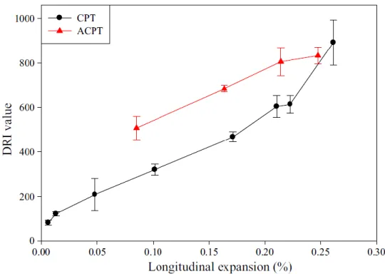
(2015b). __________________________________________________________________________ 34 Figure 16 : DRI value versus longitudinal expansion for the reactive prisms in CPT (38o_{C) and ACPT (60}o_C),

from Gautam & Panesar (2017). _______________________________________________________ 36 Figure 17 : Estimated advancement of ASR modelled using a multi-scale approach (aggregate and concrete

scale) in the concrete prisms of Lindgård et al.’s (2013a) experiments after 30 and 100 weeks of CPT exposure. The scale is a relative percentage of the theoretical advancement of ASR in absence of alkali leaching (obtained by modeling), from Multon & Sellier (2016).__________________________ 39 Figure 18 : Counting procedure proposed by Sims et al. (1992) for the QME in the case of bifurcating crack

system. The crack junctions or nodes are identified and counted. _____________________________ 48 Figure 19 : Counting of features within divided zones of the plane polished section for the CIM, from

Lindgård et al. (2004a). ______________________________________________________________ 50 Figure 20 : Features counted in the CIM under UV light: A = coarse aggregate particle containing crack(s),

AP = coarse aggregate particle containing crack(s) extending into the cement paste, P = crack in the cement paste, from Lindgård et al. (2004a). ______________________________________________ 51 Figure 21 : DRI chart showing the variability obtained by a single operator (6 replicates of the same

specimen). Mean DRI = 388 ± 25 (6%), from Grattan-Bellew & Mitchell (2006). __________________ 55 Figure 22 : A. Preparation of the concrete sections for DRI. B. Grid of 1 cm by 1 cm in size drawn on the

polished concrete section. C. Stereomicroscopic examination. _______________________________ 65 Figure 23 : Damage mapping approach. A. Damage classification for a single square (1 cm2_{). B. Example of}

a DRI damage map provided by a macro-programmed excel sheet according to the damage

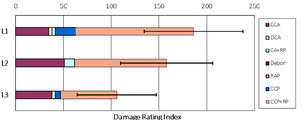
classification shown in A; the top edge of the prism is at the left. C. DRI damage map after smoothing the values using the moving average technique (the original DRI distribution for each square, i.e. before the application of the moving average technique, is provided in B). _____________________ 68 Figure 24 : Grouped lines approach - Separation of the polished concrete section in groups of two lines for

the comparison between the damage degree from the sides towards the core of the test prism. ____ 69 Figure 25 : Damage profiling approach - Separation of the polished concrete section in 4 zones for the

determination of damage profile from the top (left) to the bottom (right) of the prism. ___________ 69 Figure 26 : Petrographic features counted for the 1U-3.12 specimen during summer 2016 (1st_{DRI) and}

summer/fall 2017 (2nd _{and 3}rd_{DRI). The acronyms are defined in Table 18.______________________ 74} Figure 27 : DRI’s single operator punctual coefficient of variation (i.e. for one cm2_{) as a function of the}

specimen’s DRI number (DRI number = average punctual DRI number x 100). ___________________ 76 Figure 28 : DRI’s single operator standard deviation as a function of the specimen’s DRI number (obtained,

respectively, by multiplying the punctual standard deviation and the punctual average DRI (of

Table 28) by 100, as proposed by the DRI convention). _____________________________________ 78 Figure 29 : Statistical methodology to draw conclusions when comparing DRI values and their respective

margin of error (ME) based on a statistical approach, adapted from Ramsay & Schafer (2002).… ____ 79 Figure 30 : DRI damage map of the 6U-4.2 specimen (expansion = 0.230%). The top edge is on the left. ___ 80 Figure 31 : DRI damage map of the 1U-3.12 specimen (expansion = 0.234%). The top edge is on the left. __ 80 Figure 32 : DRI damage map of the 15U-ASTM specimen (expansion = 0.240%). The top edge is on the left. 80 Figure 33 : DRI damage map of the 3U-N.2 specimen (expansion = 0.236%). The top edge is on the left. __ 81 Figure 34 : DRI damage map of the 5U-N.2 specimen (expansion = 0.253%). The top edge is on the left. __ 81 Figure 35 : DRI damage map of the 11U-N.2 specimen (expansion = 0.120%). The top edge is on the left. _ 81 Figure 36 : DRI damage map of the 8U-4.2 specimen (expansion = 0.053%). The top edge is at the left. ___ 82 Figure 37 : DRI damage map of the 14U-4.12 specimen (expansion = 0.028%). The top edge is at the left. _ 82

(11)

xi

Figure 38 : DRI damage map of the 7U-4.2 specimen (expansion = 0.026%). The top edge is at the left. ___ 82 Figure 39 : DRI damage map of the 7U-N.2 specimen (expansion = 0.031%). The top edge is at the left. ___ 83 Figure 40 : DRI damage map of the 8U-N.2 specimen (expansion = 0.055%). The top edge is at the left. ___ 83 Figure 41 : Spatial distribution of damage (the acronyms are defined in Table 18) from the external layer

(L1) to the core (L2 & L3) of the 1U-3.12 specimen (expansion = 0.234%). The margin of error was calculated using the Equation 5. _______________________________________________________ 84 Figure 42 : Spatial distribution of damage (the acronyms are defined in Table 18) from the external layer

(L1) to the core (L2 & L3) of the 3U-ASTM specimen (expansion = 0.216%). The margin of error was calculated using the Equation 5. _______________________________________________________ 87 Figure 46 : Spatial distribution of damage (the acronyms are defined in Table 18) from the external layer

(L1) to the core (L5) of the 3U-N.2 specimen (expansion = 0.236%). The margin of error was

calculated using the Equation 5. _______________________________________________________ 89 Figure 47 : Spatial distribution of damage (the acronyms are defined in Table 18) from the external layer

calculated using the Equation 5. _______________________________________________________ 90 Figure 51 : Damage profile from the top to the bottom edges of the 6U-4.2 specimen

(expansion = 0.230%). The margin of error was calculated using the Equation 5 shown in section 3.1.2. _________________________________________________________________________________ 91 Figure 52 : Damage profile from the top to the bottom edges of the 7U-4.2 specimen

(expansion = 0.026%). The margin of error was calculated using Equation 5 shown in section 3.1.2. __ 91 Figure 53 : Damage profile from the top to the bottom edge of the 3U-N.2 specimen

(expansion = 0.236%). The margin of error was calculated using Equation 5 shown in section 3.1.2. __ 93 Figure 54 : Damage profile from the top to the bottom edge of the 5U-N.2 specimen

(expansion = 0.253%). The margin of error was calculated using the Equation 5 shown in section 3.1.2. ____________________________________________________________________________ 93 Figure 55 : Damage profile from the top to the bottom edge of the 7U-N.2 specimen

(expansion = 0.031%). The margin of error was calculated using the Equation 5 shown in section 3.1.2. _________________________________________________________________________________ 94

(12)

xii

Figure 56 : Damage profile from the top to the bottom edge of the 8U-N.2 specimen

(expansion = 0.055%). The margin of error was calculated using the Equation 5 shown in section 3.1.2. ____________________________________________________________________________ 94 Figure 57 : Damage profile from the top to the bottom edge of the 11U-N.2 specimen

(expansion = 0.120%). The margin of error was calculated using the Equation 5 shown in section 3.1.2. ____________________________________________________________________________ 94 Figure 58 : DRI results for the “fly ash comparison program”. The margin of error was calculated using the

Equation 5 shown in section 3.1.2. _____________________________________________________ 95 Figure 59 : DRI results for the “slag comparison program”. The margin of error was calculated using the

Equation 5 shown in section 3.1.2. _____________________________________________________ 96 Figure 60 : DRI weighing damage features for the “slag comparison program”. ______________________ 96 Figure 61 : Micrograph showing the presence of a reaction rim on a coarse aggregate particle of the

2U-4.2 specimen (0.026% expansion). __________________________________________________ 98 Figure 62 : Micrograph showing the presence of a reaction rim on a coarse aggregate particle of the

7U-ASTM specimen (0.025% expansion). ___________________________________________________ 99 Figure 63 : Micrograph showing the presence of a crack with reaction products in a coarse aggregate

particle (red) along with two air voids lined/filled with reaction products (yellow) in the cement paste of the 2U-4.2 specimen (0.026% expansion). ________________________________________ 99 Figure 64 : Micrograph showing the presence of an air void lined with reaction products in the cement

paste of the 10U-4.12 specimen (0.035% expansion). _____________________________________ 100 Figure 65 : Micrograph showing the presence of a crack with reaction products in a coarse aggregate

particle of the 1U-4.12 specimen (0.022% expansion). _____________________________________ 100 Figure 66 : Micrograph showing the presence of a crack with reaction products in a coarse aggregate

particle of the 7U-4.2 specimen (0.026% expansion). ______________________________________ 101 Figure 67 : Micrograph showing the presence of a crack in the cement paste (ITZ) with reaction products

for the 10U-4.12 specimen (0.035% expansion). _________________________________________ 101 Figure 68 : Micrograph showing the presence of a crack in the cement paste with reaction products for

the 2U-4.12 specimen (0.041% expansion). _____________________________________________ 102 Figure 69 : Micrograph taken from a thin section (plane polarised light) of the 4U-4.2 specimen (0.032%

expansion) showing a crack in the cement paste passing through the ITZ of a reactive aggregate particle. _________________________________________________________________________ 102 Figure 70 : Micrograph taken from a thin section (plane polarised light) of the 7U-N.2 specimen (0.031%

expansion) showing a crack in the cement paste passing through the ITZ of a reactive aggregate particle. _________________________________________________________________________ 103 Figure 71 : Zoomed view of Figure 70 (plane polarised light). ___________________________________ 103 Figure 72 : Selected zone (red square) for potassium mapping by micro XRF in the 3U-ASTM specimen

(expansion = 0.216%). ______________________________________________________________ 104 Figure 73 : First selected zone (red square) for potassium mapping with the micro XRF in the 2U-4.2

specimen (expansion = 0.026%). ______________________________________________________ 104 Figure 74 : Second selected zone (red square) for potassium mapping by micro XRF in the 2U-4.2

specimen (expansion = 0.026%). ______________________________________________________ 105 Figure 75 : Qualitative potassium map (the scale is in counts per second) showing higher potassium

concentration within a crack located in a coarse aggregate particle in the 3U-ASTM specimen

(13)

xiii

Figure 76 : Qualitative potassium map (the scale is in counts per second) showing higher potassium concentration in cracks located in the coarse aggregate particle of the 2U-4.2 specimen

(expansion = 0.026%); an overview of the selected zone is provided in Figure 73. _______________ 107 Figure 77 : Qualitative potassium map (the scale is in counts per second) showing higher potassium

concentration in a crack located in the coarse aggregate particle of the 2U-4.2 specimen

(expansion = 0.026%); an overview of the selected zone is provided in Figure 74. _______________ 108 Figure 78 : Impact of increasing the area analysed for the DRI method on the relative precision induced

by the same operator, when fixing a DRI value of 150 and 1000 in the Equation 5. ______________ 114 Figure 79 : Impact of increasing the area analysed for the DRI method on the absolute precision induced

by the same operator, when fixing a DRI value of 150 and 1000 in the Equation 4. ______________ 115 Figure 80 : Spatial distribution of damage from the external layer (L1) to the core (L3) of the 3U-3.12

specimen (the acronyms are defined in Table 18). The margin of error was calculated using the

Equation 5 shown in section 3.1.2. ____________________________________________________ 117 Figure 81 : Development of cracking due to ASR in concrete structures, from Courtier (1990). _________ 118 Figure 82 : Comparison of the DRI damage features between the 8U-N.2 and 8U-ASTM specimens. _____ 119 Figure 83 : Micrograph showing the presence of a thin (closed) crack in the cement paste for the 14U-4.12

(34 weight-% slag) specimen (0.028% expansion). ________________________________________ 126 Figure 84 : Micrograph of the 1U-4.12 (no SCMs) specimen (0.022% expansion) showing the absence of

“visible” damage features in the cement paste compared to the 14U-4.12 (34 weight-% slag)

specimen (0.028% expansion) in Figure 83. _____________________________________________ 126 Figure 85 : DRI number versus expansion (%) for the 35 concrete prisms analysed in this study. ________ 129 Figure 86 : DRI of reactive prisms in the CPT at different ages with contributions of the seven

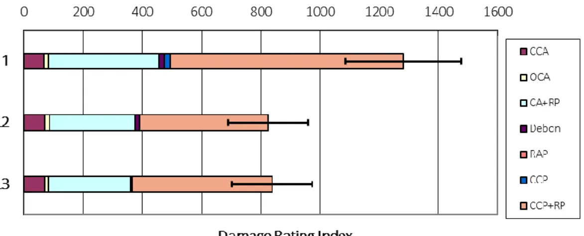
petrographic features, from Gautam & Panesar (2017). ____________________________________ 133 Figure 87 : DRI charts for 35 MPa concrete specimens incorporating ASR reactive coarse aggregates (Qc

and NM). The red bars indicate the approximate contribution of the closed cracks in aggregate (CCA) or sand particles (>1 mm) feature, adapted from Sanchez et al. (2015b) _______________________ 134 Figure 88 : Proportional contribution of the closed crack in aggregate or sand particles (> 1mm) feature

(CCA) to the global DRI number as a function of the expansion of all the prisms analysed in this study (specimens incorporating slags not included). ___________________________________________ 135 Figure 89 : Proportion of counted closed crack in aggregate or sand particles (> 1mm) feature (CCA) on

the total counted petrographic features as a function of the proportion of the CCA feature to the DRI number of all specimens analysed in this study (specimens incorporating slags not included). _____ 136 Figure 90 : DRI number versus expansion (%) of the 35 prisms analysed in this study including or not the

(14)

xiv

LIST OF TABLES

Table 1 : Some natural silicates susceptible to ASR, adapted from Rajabipour et al. (2015). ______________ 4 Table 2 : Practical applications of petrographic examination on geomaterials, from West (1995). _________ 6 Table 3: Solution data for a 33 mol% Na2O – 67 mol% SiO2 glass, from Clark & Lue Yen-Bower (1980). ____ 10 Table 4: Thermodynamic solubility limit (mM) of various SiO2 polymorphs in neutral water, from

Rajabipour et al. (2015) using data from Walther & Helgeson (1977). __________________________ 10 Table 5 : Idealized chemical compositions of “ASR gel minerals” (from Anthony et al. (1990-2003)) as

identified in ASR damaged concrete, in atoms per formula unit [apfu] and as composing oxides in weight percent, rounded to integers, from Broekmans (2012). _______________________________ 13 Table 6 : Chemical composition of the natural fine aggregate (N), crushed fine aggregate (C) and

non-reactive limestone (L) in Ramyar et al.’s (2005) study. ______________________________________ 20 Table 7: Overview of different concrete prism tests (CPTs) methods used in North America and Europe,

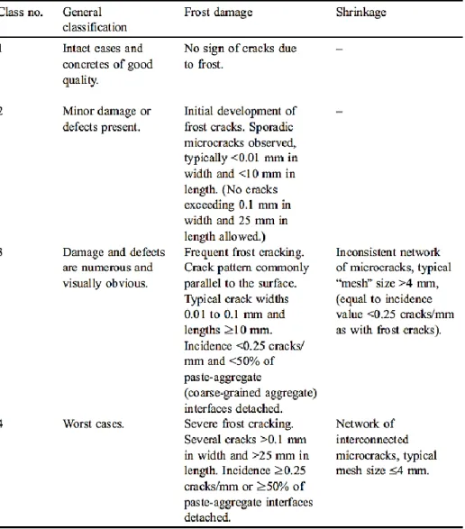
adapted from Lindgård et al. (2013b) ___________________________________________________ 24 Table 8 : Classification for the stage of ASR using polarizing microscopy, from Katayama (2017). ________ 42 Table 9 : Application of the classification shown in Table 8 for a viaduct in Japan, from Katayama (2017). _ 42 Table 10 : Damage classification and summary of the major concrete damage mechanisms observed by

Koskiahde (2004). __________________________________________________________________ 43 Table 11 : Damage Rating Number (DRN) for ASR as proposed by Broekmans (2004) (originally called

Damage rating index). _______________________________________________________________ 44 Table 12 : Damage classification from Jensen (1993) used to calculate the AAR Development Index (ADI)

developed by Hagelia (2004). _________________________________________________________ 45 Table 13 : Estimation of the K1 factor defined as the proportion of AAR affected aggregate particles,

adapted from Salomon & Panetier (1994). _______________________________________________ 46 Table 14 : Establishment of the K2 factor based on an evaluation of the extent of ASR observed at the

reaction sites, adapted from Salomon & Panetier (1994). ___________________________________ 47 Table 15 : Petrographic features counted during the QME, adapted from Sims et al. (1992) ____________ 48 Table 16 : Results of QME for evidence of ASR in concrete cores from a UK highway bridge, from Sims et

al. (1992). _________________________________________________________________________ 49 Table 17 : Results from an intra-laboratory study on the CIM performed by three petrographers, from

Lindgård et al. (2004a). ______________________________________________________________ 52 Table 18: Description of the petrographic features counted during the DRI method, adapted from Fournier

et al. (2015b). _____________________________________________________________________ 53 Table 19 : Petrographic features along with some weighing factors used in the determination of the DRI. _ 56 Table 20 : ASR damage classification for the DRI using weighing factors proposed by Villeneuve et al.

(2012), adapted from Fournier et al. (2015b) and Sanchez et al. (2017). ________________________ 57 Table 21: Overall view of the relevant (for this study) concrete prism testing laboratory conditions applied

by Lindgård et al. (2013a, 2013b & 2016b); the original testing methods are shown in Table 7. ______ 62 Table 22: Overall mix design, laboratory testing conditions and expansion attained by the prisms analyzed

in this study. ______________________________________________________________________ 63 Table 23: Petrographic features (described in Table 18) with their respective weighing factors used in the

determination of the DRI number. _____________________________________________________ 66 Table 24: Overview of the concrete prisms tested at SINTEF and of the Damage Rating Index (DRI) results.

The test specimens are classified in increasing order of expansion. ____________________________ 73 Table 25 : Overview of the single operator re-examination results. ________________________________ 74

(15)

xv

Table 26 : Overview of the global DRI results that were retained for the single (experienced) operator variability study. The results marked in red replaced the results obtained during summer 2016 as they were rejected following the single operator variability results. ___________________________ 75 Table 27 : Estimated covariance matrix considering the variability obtained for all concrete specimens

together. _________________________________________________________________________ 76 Table 28 : Estimated covariance matrix for each concrete specimen along with their respective punctual

COV (i.e. for one cm2_{). _______________________________________________________________ 76} Table 29 : Some (two-tails) z values depending on the confidence level (according to the Standard Normal

Distribution), adapted from the Student t-distribution in Ramsey & Schafer (2002). ______________ 78 Table 30 : Legend of the summary tables provided in section 3.2. _________________________________ 79 Table 31 : Comparison of the (visual) extent of damage between the edges (i.e. Zones 1 and 4) and the

middle part (Zones 2 and 3) of the conventional-size prisms with an expansion above or equal to 0.10%. The methodology applied to separate the prism in four zones is provided in Figure 25. ______ 81 Table 32 : Comparison of the (visual) extent of damage between the edges (Zones 1 and 4) and the middle

part (Zones 2 and 3) of the conventional-size prisms with an expansion below 0.10%. The

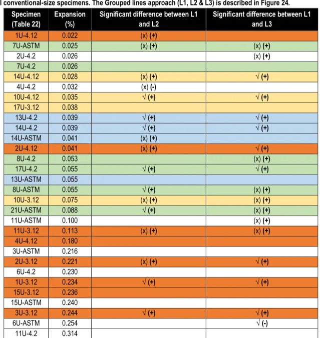
methodology applied to separate the prism in four zones is provided in Figure 25. _______________ 83 Table 33 : Comparison of the (visual) extent of damage between the external layer (Line 1) and the core

(Lines 2 and 3) of all conventional-size specimens. The Grouped lines approach (L1, L2 & L3) is

described in Figure 24. ______________________________________________________________ 85 Table 34 : Comparison of the extent of damage between the external layer (Line 1) and the core (Lines 2

and 3) of all conventional-size specimens. The Grouped lines approach (L1, L2 & L3) is described in Figure 24. _________________________________________________________________________ 88 Table 35 : Comparison of the extent of damage between the edges (Zones 1 and 4) and the middle part

(Zones 2 and 3) of the conventional-size prisms using the Damage profile approach. The latter is described in Figure 25. ______________________________________________________________ 92 Table 36 : Experimental program to compare damage in specimens with and without fly ashes. _________ 95 Table 37 : Experimental program to compare damage in specimens with and without slags. ____________ 95 Table 38 : Detailed DRI results (weighing factors according to Villeneuve et al., 2012) for the 1U-4.12

specimen (Spratt aggregate; expansion of 0.022%). The acronyms are defined in Table 18. It is to be noted that the RR and RPV features are not considered in the calculation of the DRI. _____________ 98 Table 39 : Detailed DRI results (weighing factors according to Villeneuve et al. (2012) for the 7U-ASTM

specimen (Ottersbo aggregate; expansion of 0.025%). The acronyms are defined in Table 18. It is to be noted that the RR and RPV features are not considered in the calculation of the DRI. ___________ 98 Table 40 : Margin of error calculated for each specimen (Table 26) of the variability study using the

Equation 5 shown in section 3.1.2 (with the whole area). __________________________________ 113 Table 41 : Summary of the results provided in Table 34 when comparing the extent of damage within the

core and the external layer of the alkali wrapped specimens (either with or without SCMs) (grouped lines approach). The color code is detailed in Table 30. ____________________________________ 117 Table 42 : Comparison of the results obtained with the DRI damage mapping (Table 31 and Table 32) and

the damage profile (Table 35) tools for assessing the difference in damage between the top edge (zone 1) and the middle part (Zones 2 and 3) of the conventional-size specimens. _______________ 122 Table 43 : Comparison of the results obtained with the DRI damage mapping (Table 31 and Table 32) and

the damage profile (Table 35) tools for assessing the difference in damage between the bottom edge (zone 4) and the middle part (Zones 2 and 3) of the conventional-size specimens. _______________ 123

(16)

xvi

Table 44 : Comparison of the results obtained with the DRI damage map (Table 33) and the investigation of grouped lines (Table 34) for assessing the difference in damage between the external layer (L1) and the core (Lines L2 and L3) of the conventional-size specimens.___________________________ 124 Table 45 : DRI contribution of the closed crack in aggregate or sand particles (> 1mm) feature (CCA) for

specimens with an expansion close to or lower than 0.040 % (specimens incorporating slags not included). The margin of error was calculated with a 95% confidence interval of the mean. _______ 135 Table 46 : Petrographic features along with their respective weighing factors recommended for the

determination of the DRI following this study. ___________________________________________ 143 Table 47 : ASR damage classification for the DRI using weighting factors proposed after this study based

(17)

xvii

REMERCIEMENTS

Ce projet de recherche n’aurait jamais été possible sans l’immense support de mon directeur de recherche Prof. Benoit Fournier et de ma codirectrice de recherche Prof. Josée Duchesne. Je tiens donc à les remercier en guise de reconnaissance à la grande contribution qu’ils ont eu sur mon cheminement lors des deux dernières années. De plus, je tiens à remercier le personnel du Service de consultation statistique (SCS) de l'Université Laval pour souligner leur importante contribution au projet, dont deux membres en particulier, soit Sergio Ewane Ebouele et Mahukpe Narcisse Ulrich Singbo. Je veux aussi remercier tous mes collègues de bureau, soit Anthony Allard, Isabelle Fily-Paré, Jean-Benoit Darveau, Alexandre Rodrigue, Frédéric Béland et Cédric Drolet, qui ont toujours été présents pour répondre à mes questions ou m’aider dans mes travaux de laboratoire. Je me dois également de remercier particulièrement ma collègue Mélissa Roy-Tremblay pour tout le travail consacré à développer les outils informatiques d’analyse spatiale nécessaires à la réalisation de ce projet. Je veux remercier et souligner tout le travail accompli par les auxiliaires de recherche au premier cycle, plus particulièrement Samuel Couture, Thomas Duplessis et Edgardo Alvarado, qui ont grandement contribué à l’accomplissement de ce projet. Je veux aussi remercier Prof. Leandro Sanchez pour ses judicieux conseils lorsque j’en ai eu besoin et pour avoir accepté d’évaluer mon séminaire de maîtrise.

Je tiens à remercier des gens qui me sont chers et qui ont eu un rôle capital dans le succès de mes études depuis leur début. Je pense à mes parents qui m’ont toujours supporté dans mes projets et qui n’ont jamais douté de moi. Également, je me sens privilégié par la vie de partager mon quotidien avec une femme exceptionnelle qui a accepté de vivre avec moi les joies et les embûches d’un tel projet de vie, soit les études graduées. Une telle vocation se doit d’être vécue à deux et ma partenaire de vie Loïze Maréchal a toujours su être compréhensive et dédiée tout autant que moi à ce projet de recherche. Je suis extrêmement reconnaissant de l’incroyable support que Loïze a su m’accorder tout au long de ces deux années. Le crédit qui lui revient pour la réalisation de ce projet ne sera jamais reconnu à sa juste valeur.

En terminant, je me permets de souligner l’aide de mes collègues pour leur support dans la réalisation de mes tâches associées au chapitre étudiant ACI@UL, puisque leur travail mérite d’être reconnu comme il se doit. Alors, je dois dire un grand merci à Pierre Siccardi, Frédéric Béland, Mélissa Roy-Tremblay, Alexandre Rodrigue, Gilberto Cidreira Keserle, Juliano Provete Vincler, Thomas Jacob-Vaillancourt et Frédéric Bédard.

I wish to personally thank M. Jan Lindgård who made this project possible by sending us the specimens that were analysed in this study, but mostly for all the generous time spent helping me with questions regarding the COIN project. I would also like to thank SINTEF for all the financial support dedicated to this project.

(18)

1

INTRODUCTION

This MSc dissertation summarizes the results of quantitative damage assessments using the Damage Rating Index method and petrographic analyses of 35 concrete prisms that have been subjected to laboratory testing as part of the COIN program Part I (Lindgård et al., 2013a, 2013b) and Part II (Lindgård et al., 2016b). Two methods were used to assess damage in the above concrete specimens, i.e. Damage Rating Index (DRI) and Image Analysis (IA). The reported MSc project focuses on the DRI results while another Master student (Mélissa Roy-Tremblay) carried out damage assessments using the IA method.

General context of the study

Alkali-aggregate reaction (AAR) is a harmful chemical reaction between certain aggregate constituents and the alkali hydroxides of the cement paste pore solution, which can eventually lead to an important cracking network in the affected concrete. It is one of the main deleterious processes affecting the durability of concrete structures worldwide (Fournier & Bérubé, 2000); a map of AAR occurrences is shown in Figure 1. Over the past few decades, research has been carried that led to improvements of the aggregate performance test methods in such a way that potential alkali-reactivity of aggregates can generally be reliably assessed prior to their use in concrete (e.g. RILEM Technical Committee 219-ACS, 2016)). However, many structures were built with reactive aggregates before the risk posed by AAR was adequately recognised (Dunant & Bentz, 2012). Such concrete structures need to be assessed from durability and, in severe cases, from structural point of views. This can be challenging for engineers because the rate and extent of cracking can vary significantly from an affected structure to another and even among elements of a single structure (Wood & Johnson, 1993). Since compressive strength is not necessarily a good indicator of the condition of concrete damaged by AAR (Giaccio et al., 2008; Sanchez et al., 2017), engineers need suitable tools and procedures to assess the current condition (diagnosis) and the potential for further expansion/distress (prognosis) of concrete damaged by AAR (Sanchez et al., 2015a; 2015b).

Different techniques have been proposed in the past for assessing damage in concrete due to AAR, one of them being the Damage Rating Index (DRI) method developed by P.E. Grattan-Bellew from the National Research Council of Canada (Grattan-Bellew & Danay, 1992). The DRI is a petrographic tool performed with the use of a stereomicroscope (about 15x magnification) where damage features generally associated with alkali-silica reaction (ASR) are counted by an operator through a 1 to 1.5 cm² grid drawn on the surface of a polished section. This technique is increasingly being used in North America. However, there is currently no standard test procedure for the method, making it difficult to compare results from different research laboratories. Furthermore, even if the DRI can reliably assess damage in concrete affected by AAR (Sanchez et al., 2015b & 2017), applying this tool to identify various damage variations within the same concrete specimen/component is still largely

(19)

2

unexplored. This potential application highly depends on the “sensitivity” of the method since it necessitates comparing small areas of the same polished section.

Figure 1 : World map showing countries with known cases of deleterious AAR (black color), but “incomplete” because it is in constant evolution, from Broekmans (2012).

Several research projects have been carried out at Laval University by Professor Marc-André Bérubé, Josée Duchesne and Benoit Fournier and their respective research teams to evaluate the applicability and the efficiency of the DRI method as a damage assessing tool for concrete. For instance, Smaoui et al. (2004a; 2004b) tested the DRI for assessing damage in a field structure and compared results with other techniques. Then, an intra-laboratory study was conducted (Villeneuve et al., 2012), followed by an evaluation of its reliability for damage assessment in concrete of different strengths and incorporating a range of reactive aggregates (Sanchez et al., 2015b; 2017). Moreover, the method was performed to assess the global condition of the concrete of different ASR-affected structures/structural components like bridges (Fournier et al., 2009; 2015a; Thomas et al., 2013a; 2013b; Fournier, 2016; Fournier & Champagne, 2016), dams (Grattan-Bellew, 2005; Fournier & Bérubé, 2011; Thomas et al., (2012); Fournier, 2014), locks (Lamothe & Fournier, 2009), thick slabs (subjected to accelerated laboratory conditions) (Allard et al., 2016), concrete pavements (Tremblay et al., 2012) and a tunnel (Tremblay & Fournier, 2011). One of the objectives behind all this work was to show the reliability of the DRI method to assess the damage of concrete affected by AAR. This project was dedicated to the same purpose; however, it focused mainly on appraising the “sensitivity” of the DRI method.

(20)

3

1. LITERATURE REVIEW

1.1 Alkali-aggregate reaction (AAR)

Globally, AAR can be summarized as follows: ‘susceptible minerals’ react under high alkaline environment and high moisture conditions to generate a hydrophilic product which induces internal pressure and ultimately causes cracking of the concrete as a whole (Broekmans, 2012). Depending on the reactive minerals present, two different types of AAR can occur: the alkali-carbonate reaction (ACR) and the alkali-silica reaction (ASR) (Fournier & Bérubé., 2000). The first is often referred to “the so-called ACR” because it is still a highly controversial topic (Jensen, 2012; Poole & Sims, 2016). The second is by far the most common form of AAR and lots of research has been carried out since this phenomenon (that later became known as ASR) was reported the first time by Thomas Stanton in 1940 (Stanton, 1940). This review is focussing only on ASR because none of the concrete specimens analysed in this study were affected by ACR.

1.1.1 Alkali-silica reaction (ASR)

The ASR is characterized by the breakdown of silanol bonds within certain types of silica minerals found in some aggregates by the alkali hydroxides from the concrete pore solution (Dunant & Scrivener, 2012). Strained quartz can also be thermodynamically unstable due to its high free energy in its crystalline network after a certain degree of deformation (Ponce & Batic, 2006). Forms of reactive silica were listed in the following decreasing order of reactivity by Broekmans (2012):

1. Opal (SiO2 ∙ nH2O), 2. Moganite (SiO2), 3. Chalcedony (SiO2),

4. Fine-grained quartz (SiO2) (i.e. chert,and flint, but also siltstone) , 5. Coarse-grained quartz (SiO2).

Further information regarding natural silicates susceptible to ASR is provided in Table 1. The reactive silica progressively forms silicate complexes leading to the formation of a viscous and hygroscopic product called “ASR gel” (Fournier & Bérubé, 2000). The gel has the capacity to bind water molecules and other ionic species of the pore solution causing it to swell. The low permeability of the concrete limits swelling of the gel and locally exert pressure at sites of expansive reaction (Fournier & Bérubé, 2000). The pressure is resisted by the concrete until exceeding its tensile strength (Bazant & Steffens, 2000), which leads to cracking of the aggregate particles and of the surrounding cement paste, eventually forming a network between reactive particles when damage

(21)

4

increases (Sanchez et al., 2015b). According to St. John et al. (1998), Fournier & Bérubé (2000) and Thomas et al. (2013c), there are three essential requirements for ASR:

• A reactive aggregate must be present,

• The concentration of alkali hydroxides (Na-_{, K}-_{, OH}-_{) in the pore solution must be high enough,} • Sufficient moisture must be present (≈ > 80-85 % RH).

Table 1 : Some natural silicates susceptible to ASR, adapted from Rajabipour et al. (2015).

Name Description Example rock types

Opal Amorphous silica: a form of highly

condensed silica gel (contains 4-9% water); always highly reactive

Occurs as primary or secondary mineral in rocks such as chert, flint, shale, limonite, sandstone, rhyolite, marl and basalt

Volcanic glass (e.g. Obsidian) Reactive in some cases Common minor constituent of fine-grained volcanic rocks such as basalt, rhyolite, andesite Cristobalite and trydimite High-temperature polymorphs of SiO2;

stable only at high temperature, but can crystallize and persist meta-stably at lower temperatures

Cryptocrystalline (fine grained) quartz and other fibrous silica (e.g. chalcedony)

Moderately reactive Constituents in rocks such as cherts and flints and as cementing material in greywacke

Highly crystalline silica Embedded in other minerals Mylonite Strained quartz Only mildly reactive but degree of reactivity

increases with strain

Quartzite

1.1.2 Diagnosing ASR

Different guides for the identification and appraisal of ASR in concrete field structures were prepared over the past few decades (e.g. British Cement Association (BCA), 1992; Institution of Structural Engineers (ISE), 1992; CSA A864, 2000; Larbi et al., 2004; Bérubé et al., 2005b; Fournier et al., 2010; Thomas et al., 2011a; 2013c; Godart et al., 2013). In general, the first stage consists in identifying the cause of deterioration and to assess the current condition of the concrete (diagnosis). This section focuses on identifying the source of deterioration as assessment of the concrete condition is discussed in section 1.5. For this purpose, a complete investigation program is recommended, which usually consists of a visual inspection of the structure and a laboratory investigation performed on extracted cores. The objective of the visual inspection is 1) to provide a preliminary evaluation of the nature, the extent and the progress (with repeated inspections over time) of any deterioration affecting the concrete structure; and 2) identify areas that might require further investigations and/or immediate

(22)

5

actions (Fournier et al., 2010). Besides, it is important to note that the source of distress (e.g. ASR, thaumasite sulfate attack (TSA), delayed ettringite formation (DEF), freeze-thaw, etc.) generally cannot be confirmed during the visual inspection, so sampling the structure is required/essential. According to most guides, the best approach to confirm the cause of deterioration is by petrographic examination of the extracted concrete cores. Petrographic examination of concrete is a generic term that can be described as ”application of geoscience methods to study concrete” since geomaterials can, to a certain extent, be studied in the same way as minerals and rocks are evaluated (West, 1995). This term is related to petrography, which can be defined as ”the art of describing a rock” based on an evaluation of its texture and mineralogy using geoscience methods such as visual investigation, X-Ray Diffraction (XRD), Scanning Electron Microscopy (SEM), Electron Microprobe (EPMA), polarized light microscopy, Raman microscopy, etc. (Fernandes et al., 2009). However, it should be noted that “concrete petrography”, in practice, gradually became equivalent to “thin section analysis” (Fernandes et al., 2009); on the other hand, petrographic examination can involve any geoscience methods (including thin section). A list of practical applications of petrography to study concrete is provided in Table 2.

Petrographic examination of concrete was used locally in the 1960’s (e.g. Idorn, 1967) and was found to be highly usefull to the concrete industry (Erlin & Stark, 1990). As a result, it was noticed that petrography could definitely become handy for characterizing different ‘phases’ in concrete and the first standard pratice for petrographic examination of hardened concrete was then developed (ASTM C856, 1977). Several authors consider petrographic examination as an essential tool to identify and characterize (mostly in terms of morphology and chemistry) different phases in damaged concrete (e.g. Leroux & Cador, 1984; Erlin & Stark, 1990; St. John, 1990; Sims et al., 2004; Broekmans, 2009; Fernandes, 2009; Fernandes et al., 2009; Poole & Sims, 2016). Moreover, many authors used petrographic examination to identify the source of distress in concrete structures affected by different pathologies, such as ASR (e.g. Sims et al., 2004; Walker et al., 2006; Ekolu, 2009; Fernandes, 2009; Fernandes et al., 2013), fire (Ingham, 2009), acid attack (Fernandes et al., 2012), TSA (e.g. Eden, 2003; Hou & Daugherty, 2011), oxidation of sulfide-bearing aggregates (Rodrigues et al., 2012), DEF (e.g. Sahu & Thaulow, 2004; Sims et al., 2004; Thomas et al., 2008) and radioactivity (Buck, 1988).

(23)

6

Table 2 : Practical applications of petrographic examination on geomaterials, from West (1995).

Usually, the presence of ASR is identified by visual examination of concrete cores. At this stage, the petrographer has to identify distress features generally associated with ASR (Fournier et al., 2010; Sims et al. 2016). This can be done at different scales depending on the resolution of the microscope used (if any). Inside the concrete element (i.e. ≈ > 10 cm from the surface, but variable), ASR is characterized by the presence of a somewhat regular cracking network that runs through the reactive (coarse and/or fine) aggregate particles and the cement paste (Figure 2) and whitish or translucent secondary reaction products filling the cracks or air voids of the

(24)

7

cement paste (Figure 3A) at the macro scale or under a stereomicroscope (≈5-100x), and most likely colorless and amorphous when using an optical microscope (≈10-400x) (Figure 3B). Concrete specimens can also be examined at a much smaller scale (≈ 1-10 μm) using a SEM\EPMA that can allow qualitative or quantitive chemical analysis. Under a SEM, ASR is characterized by the occurrence of either massive or “textured” (e.g. botryoidal or reticular surface microtexture) reaction products (Figure 3C), or crystalline “rosette-like” reaction products (Figure 3D) (Bérubé & Fournier, 1986; Leemann et al. 2016). For this project, even though concrete can be studied at virtually any scale, it was decided to work at the microscopic scale only using a stereomicroscope (≈15x).

Figure 2 : Cracking pattern in concrete affected by ASR originating (a) from the fine aggregate fraction and (b) from the coarse aggregate fraction, from BCA (1992).

1.2 ASR distress mechanism

The global ASR distress mechanism is well understood in its major steps and was described in Section 1.1.1. However, despite decades of investigations, the current state of knowledge about the physical and chemical aspects of the ASR damage generation mechanisms remains somewhat limited, especially at the molecular to micro-scale levels (Rajabipour et al., 2015). This is a considerable issue for the development and application of numerical modeling to predict the behaviour of structures affected by ASR. According to Dunant & Scrivener (2010), such numerical models are either formulated from phenomenological or mechanistic points of views, and the lack of consensus about the origin of the degradation mechanism makes the formulation of experimentally based mechanistic models arduous, because they rely on underlying hypotheses about the degradation mechanism. Consequently, mechanistic modelling is an underused approach that could potentially lead to good results if the distress mechanism was better known.

(25)

8

A B

C D

Figure 3 : Petrographic features of ASR observed at different scales: (A) Concrete under a stereomicroscope (the line is ≈ 1cm), from Fournier et al. (2015b). (B) Thin section under an optical microscope with plane polarized light, from Poole & Sims (2016). (C, D) Concrete under a SEM equipped with an energy-dispersive X-ray analyser, from Bérubé & Fournier (1986).

(1)

According to the authors, a highly degraded (SiO2)solid may also transform directly into (SiO2)gel, as long as sufficient but not excessive cross-linking is maintained between silica chains. However, the thermodynamic and kinetic aspects of the above reaction remain poorly understood as there are many parameters to consider (e.g. aggregate composition and heterogeneity, local pore solution composition at silica surface, temperature, humidity, etc.).

There still is some debate around whether or not the reactive silica is dissolved prior to the formation of ASR reaction products, but most authors tend to say that it does (Rajabipour et al., 2015). The dissolution of silica in water actually occurs in “normal” environmental conditions (i.e. ≈ 25°C and pH ≈ 6), tough at a much slower rate than in “concrete conditions” (Hamilton et al., 2000; Brantley, 2008). This phenomenon, often reffered to “glass corrosion”, has been studied for over a century in the laboratory (e.g. Walther & Helgeson, 1977; Hench, 1978; Clark & Lue Yen-Bower, 1980; Dent Glasser & Kataoka, 1981; Scholze, 1982; Bunker, 1994; Tournié et al., 2008). As a result, it is fairly well understood that the solubility of silica increases with pH (Table 3) and temperature (Table 4). However, the (undesired) dissolution of silica in concrete aggregates that results in deleterious ASR is not understood to the same extent because the properties of alkali-reactive forms of silica in different rock types are rarely known to the same extent as the “types of silica” used in dissolution experiments. Furthermore, the solubility of silica is affected by the presence of other dissolved species in the concrete pore solution (Broekmans, 2012). For instance, Curtil et al. (1992) noticed that a pore solution containing calcium would dissolve less opal than a calcium-free pore solution of the same pH, and a similar finding was reported by Chatterji (1979) and Chatterji & Clausson-Kass (1984). On the other hand, the presence of alkalis in the pore solution helps weakening the siloxane bonds, and therefore increases the solubility of reactive silica (Dove et al., 2008).

(27)

10

Table 3: Solution data for a 33 mol% Na2O – 67 mol% SiO2 glass, from Clark & Lue Yen-Bower (1980).

* SA/V = glass surface area-to-solution volume ratio

solid (2)

OH-_{then continue to attack the Q}₃_{to form silicate ions and small polymers (Garcia-Diaz et al., 2006):}

(SiO

_5/2-

)

aq

+ (OH

-

₎

aq

+ 1 2

⁄ H

2

O → (H

2

SiO

42-

)

)

Afterwards, the silicate ions bind with cations of the pore solution to polymerize and form complexes (sol/gel), most likely C-S-H and/or C-K-S-H and C-N-S-H phases (Garcia-Diaz et al, 2006). It is important to note that the Ca ions are essential for these processes to occur. In the absence of Ca ions, the dissolved species remain in solution, thus preventing deleterious expansion due to ASR to occur (Chatterji, 1979; Wang & Gillot, 1991; Bleszynski & Thomas, 1998; Thomas, 1998; Gaboriaud et al., 1999). However, this is unlikely to happen in Portland cement concrete, because portlandite can dissolve to compensate the calcium uptake through the formation of the ASR products. Once a nucleus of critical size is formed, it grows to nano-colloidal silica sol

Applying the Damage Rating Index for the spatial damage assessment in concrete specimens affected by alkali-silica reaction (ASR)

© Mathieu Champagne, 2020

Applying the Damage Rating Index for the spatial

damage assessment in concrete specimens affected by

alkali-silica reaction (ASR)

Mémoire

Mathieu Champagne

Maîtrise interuniversitaire en sciences de la Terre - avec mémoire

Maître ès sciences (M. Sc.)

Applying the Damage Rating Index for the spatial

damage assessment in concrete specimens affected by

alkali-silica reaction (ASR)

Mémoire

Mathieu Champagne

Sous la direction de :

Benoît Fournier, Directeur de recherche

Josée Duchesne, Codirectrice de recherche

RÉSUMÉ

ABSTRACT

CONTENTS

LIST OF FIGURES

LIST OF TABLES

REMERCIEMENTS

INTRODUCTION

General context of the study

1. LITERATURE REVIEW

1.1 Alkali-aggregate reaction (AAR)

1.1.1 Alkali-silica reaction (ASR)

1.1.2 Diagnosing ASR

1.2 ASR distress mechanism

1.2.1 Chemical aspect

(SiO

)

↦

(SiO

)

↦

(SiO

)

↦

(SiO

)

↦

swelling of gel

2(SiO

)

+ (OH

)

→ (SiO

)

+ (SiO

H)

(SiO

)

+ (OH

)

+ 1 2

⁄ H

O → (H

SiO

)

(SiO

H)

+ 3(OH

)

→ (Si(OH)

)

⟷ (H

SiO

)

+ (H

)

⟷ (H

SiO

)

+ 2(H

)

₎

₎