Learning from positive and unlabeled examples in biology

HAL Id: pastel-00566401

https://pastel.archives-ouvertes.fr/pastel-00566401

Submitted on 16 Feb 2011

HAL is a multi-disciplinary open access archive for the deposit and dissemination of sci-entific research documents, whether they are pub-lished or not. The documents may come from teaching and research institutions in France or abroad, or from public or private research centers.

L’archive ouverte pluridisciplinaire HAL, est destinée au dépôt et à la diffusion de documents scientifiques de niveau recherche, publiés ou non, émanant des établissements d’enseignement et de recherche français ou étrangers, des laboratoires publics ou privés.

Learning from positive and unlabeled examples in

biology

Fantine Mordelet

To cite this version:

Fantine Mordelet. Learning from positive and unlabeled examples in biology. Bioinformatics [q-bio.QM]. École Nationale Supérieure des Mines de Paris, 2010. English. �NNT : 2010ENMP0058�. �pastel-00566401�











École doctorale n

432 :

Sciences des métiers de l’ingénieur

Doctorat européen ParisTech

T H È S E

pour obtenir le grade de docteur délivré par

l’École nationale supérieure des mines de Paris

Spécialité « Bio-informatique »

présentée et soutenue publiquement par

Fantine MORDELET

le 15 décembre 2010

Méthodes d’apprentissage statistique à partir d’exemples positifs

et indéterminés en biologie.

∼ ∼ ∼

Learning from positive and unlabeled examples in biology.

Directeur de thèse : Jean-Philippe VERT

Jury

François DENIS,Professeur, Laboratoire d’Informatique Fondamentale, Université de Provence Rapporteur

Yves MOREAU,Professeur, Bioinformatics Research Group, Université de Leuven (Belgique) Rapporteur

Florence D’ALCHE-BUC,Professeur, Laboratoire IBISC, Université d’Evry-Val d’Essonne Examinateur

Denis THIEFFRY,Professeur, Département de Biologie IBENS, Ecole Normale Supérieure Examinateur Jean-Philippe VERT,Maître de recherche, Centre de Bio-Informatique, Mines ParisTech Directeur de thèse

MINES ParisTech Centre de Bio-Informatique

Contents

1.1.1.2 Why study gene regulation? . . . 4

1.1.1.3 Experimental characterization . . . 6

1.1.1.4 In silico inference . . . 8

1.1.2 The disease gene hunting problem . . . 14

1.1.2.1 Disease gene discovery . . . 14

1.1.2.2 Experimental approaches for disease gene iden-tification . . . 14

1.1.3 Data resources . . . 17

1.1.3.1 Transcriptomics data . . . 19

1.1.3.2 Subcellular localization data . . . 21

1.1.3.3 Sequence data . . . 21

1.1.3.4 Annotation data . . . 22

1.1.3.5 Data fusion . . . 25

1.2 Machine learning context . . . 25

1.2.1 Learning from data . . . 26

1.2.1.1 Unsupervised versus supervised learning . . . 26

1.2.1.2 The bias-variance trade-off . . . 26

1.2.1.3 Some variants of supervised learning . . . 28

1.2.2 The Support Vector Machine . . . 32

1.2.2.1 A geometrical intuition . . . 32

1.2.2.2 Soft margin SVMs . . . 35

ii CONTENTS

1.2.2.3 Non-linear SVMs . . . 37

1.2.3 Kernels methods . . . 38

1.2.3.1 Motivations . . . 38

1.2.3.2 Definitions . . . 38

1.2.3.3 The kernel trick . . . 39

1.2.3.4 A kernelized SVM . . . 40

1.2.3.5 Data fusion with kernels . . . 42

1.3 Contributions of this thesis . . . 44

1.3.1 A bagging SVM to learn from positive and unlabeled examples . . . 44

1.3.2 Regulatory network inference . . . 45

1.3.3 Identification of disease genes with PU learning . . . . 45

2 A bagging SVM for PU learning 47 2.1 R´esum´e . . . 47

2.2 Introduction . . . 48

2.3 Related work . . . 50

2.4 Bagging for inductive PU learning . . . 51

2.5 Bagging SVM for transductive PU learning . . . 53

2.6 Experiments . . . 55

2.6.1 Simulated data . . . 55

2.6.2 Newsgroup dataset . . . 57

2.6.3 E. coli dataset : inference of transcriptional regulatory network . . . 61

2.7 Discussion . . . 62

3 Regulatory network inference 65 3.1 R´esum´e . . . 65

3.2 Introduction . . . 66

3.3 System and Methods . . . 68

3.3.1 SIRENE . . . 68

3.3.2 SVM . . . 69

3.3.3 Choice of negative examples . . . 70

3.3.4 CLR . . . 71

3.3.5 Experimental protocol . . . 71

3.4 Data . . . 73

3.5 Results . . . 74

4 Prioritization of disease genes 79 4.1 R´esum´e . . . 79

CONTENTS iii

4.3 Related work . . . 82

4.4 Methods . . . 86

4.4.1 The gene prioritization problem . . . 86

4.4.2 Gene prioritization for a single disease and a single data source . . . 86

4.4.3 Gene prioritization for a single disease and multiple data sources . . . 88

4.4.4 Gene prioritization for multiple diseases and multiple data sources . . . 89

4.5 Data . . . 93

4.5.1 Gene features . . . 93

4.5.2 Disease features . . . 93

4.5.3 Disease gene information . . . 93

4.6 Results . . . 94

4.6.1 Experimental setting . . . 94

4.6.2 Gene prioritization without sharing of information across diseases . . . 95

4.6.3 Gene prioritization with information sharing across dis-eases . . . 96

4.6.4 Is sharing information across diseases beneficial? . . . . 98

4.6.5 Predicting causal genes for orphan diseases . . . 102

4.7 Discussion . . . 102

Conclusion 107

Remerciements

Je tiens tout d’abord `a remercier M. Y. Moreau, F. Denis, D. Thieffry et Mme F. D’Alch´e-Buc pour avoir accept´e d’ˆetre membres de mon jury de th`ese et de faire ainsi partie de la dizaine de personnes qui aura lu cette th`ese (ce qui comprend d´ej`a mon humble personne et mon directeur de th`ese). Ce qui m’am`ene tout naturellement `a remercier le directeur de th`ese sus-mentionn´e et Emmanuel Barillot, le directeur de l’u900 pour m’avoir accueillie dans cette belle ´equipe. Jean-Philippe, en vertu de tout ce que tu m’as apport´e, je te souhaite d’´elever plein d’autres petits CBIO, qui baigneront d`es la prime enfance de leur carri`ere de chercheur dans la douce id´eologie du grand noyau.

Ensuite, il y a mes coll`egues, qui ont aussi jou´e un rˆole crucial dans mon apprentissage.. Quelle consolation de les avoir quand on doute, quand les choses ne marchent pas si bien qu’on aimerait (et ¸ca arrive souvent!). Et puis c’est comme quand on est petit, que les vacances se terminent et qu’on est triste de retourner `a l’´ecole mais on sait quand mˆeme qu’on sera content de revoir les copains. Sauf qu’`a l’´epoque, on ne racontait pas des blagues foireuses en buvant du caf´e d`es le matin. La liste est longue mais on va essayer de ne pas oublier de monde. Pr´ecisons aussi que certains peuvent se trouver dans plusieurs cat´egories mˆeme je ne cite leur nom qu’une fois. Commen¸cons par les curistes. Il y a mes cops de Martini: Laurence, Fanny, Jenny, Loredana et les deux accolytes de mon “trio des th´esardes”: C´ecile et Anne. Sur le plan de la logistique, elles sont super aussi, elles ont tou-jours le dentifrice, le maillot de sport ou le cachet qui me manque (mˆeme si le Spasfon ne fait pas grand chose contre l’appendicite). Il y a ceux de la cantine de l’ENS : Gautier, Patrick, St´ephane et St´ephane, Nicolas, Jonas, Caroline, Isabel, Joern avec qui on a bien rigol´e pour oublier le goˆut des aliments qu’on y sert. Il y a tous ceux que j’ai harcel´e pour des questions diverses et qui m’ont r´epondu avec gentillesse: comment marche un ordi avec Pierre et Stuart, la biologie avec Simon, Perl et bash avec S´everine et Georges (vous ne vous en souvenez pas forc´ement mais moi si). Et mes patients col-l`egues de bureau qui r´epondent invariablement “`a tes souhaits” `a tous mes

vi REMERCIEMENTS

´eternuements et Dieu sait qu’il en faut de la constance pour tenir le rythme : Bruno, Valentina et Paola. Une mention sp´eciale `a Pierre N. qui m’a initi´e au monde de la bioinfo; il a ´et´e mon professeur, puis il m’a aid´ee `a trouver un stage de c´esure et enfin, il m’a fait d´ecouvrir Curie quand je cherchais un endroit o`u passer trois merveilleuses ann´ees de th`ese, ¸ca tombait bien, non?. Maintenant, on passe au CBIO. Pr´ecisons tout de suite que le CBIO, c’est bien et que tout le monde devrait en ˆetre convaincu. Il y a les grands pontes de la secte (euh, du labo) qui ont toujours de bons conseils, ˜A˘a savoir, “un bon chercheur doit toujours ˆetre un peu malheureux, avoir un peu faim et un peu froid” et toutes ces choses indispensables pour bien commencer une carri`ere : V´eronique, Yoshi et Jean-Philippe. Il y a mes “grands fr`eres” de th`ese : Laurent, Franck, Misha, Kevin et Martial. Ils m’ont appris la fenˆetre noire (enfin, le terminal comme il paraˆıt qu’il faut dire), le cluster, me servir d’un Mac, la r´egularisation (“plus C est grand, plus... c’est quoi d´ej`a?”), v´en´erer notre chef et tellement d’autres choses. Et tout ¸ca m’a servi ensuite pour accueillir ma “petite soeur” de th`ese : Anne-Claire, mais l’´echange a eu lieu dans l’autre sens aussi de bien des mani`eres.

Passons `a mes amis, on ne peut pas dire, il en faut dans la vie! Pour suivre assidˆument les p´erip´eties, les amours, les emmerdes de sa Cocotte depuis pr`es de 10 ans, il y a Poulette (ou encore Nathalie) qui me soutient `a coups de cocktails ou s´eances de Desperate Housewives avec tisane et chocolat, selon l’humeur. Pour remettre un peu de sport dans cette vie de d´epravation, tout en papotant bien sˆur, il y a C´elinou (qui ne recule pas devant un petit cock-tail non plus). Elle appartient aussi `a la cat´egorie “copains th´esards”, ceux qui savent de quoi il retourne et qui peuvent mieux que quiconque appr´ecier les joies et les peines de cette situation : Maxime, Tim , Magali, R´emi et Matthieu. Cependant, il serait injuste de ne pas mentionner les autres, qui suivent mes progr`es malgr´e tout et qui sont sont pr´esents quand il le faut, tout simplement: Nadia et Laurent, les Despos, les Saint-Louisards, les Ensae, et enfin mes amis de lyc´ee, coll`ege et primaire que j’ai retrouv´es tout r´ecemment.

A pr´esent, place `a une cat´egorie toute particuli`ere : ma famille. Ils ont eu d’autant plus de m´erite de me soutenir qu’ils n’avaient la plupart du temps aucune id´ee de ce que je faisais, avouons-le! Je voudrais donc exprimer ma reconnaissance et ma tendresse `a Mamie de Bretagne, `a mes oncles et tantes : Patrick, Laurence et Thierry `a mes cousins et cousinettes : Caroline, Emilie, Victor et J´er´emie. Ensuite bien sˆur, `a mes soeurs, Manon et Oriane, qui elles aussi d´efendent vaillament les couleurs des Mordelet dans la jungle des ´etudes sup´erieures. Mˆeme si techniquement, ils ne sont pas de ma famille, ils le sont `a mes yeux, merci `a Alain et Laurence, `a mon parrain ador´e Denis

vii

et sa femme Agn`es chez qui je peux toujours recharger mes batteries. A ce stade, et sans pour autant verser dans Zola, il est temps d’adresser une pens´ee affectueuse `a mon p`ere, qui je l’esp`ere aurait ´et´e fier de moi. Enfin, last but not least, Mˆoman! Elle a toujours ´et´e l`a dans mes grands moments de doute, pour me donner confiance et y croire `a ma place. Ca a commenc´e la veille de ma rentr´ee en CP: “J’y arriverai jamais Maman... C’est trop dur le CP!” et ¸ca a continu´e ainsi jusqu’`a la th`ese, c’est dire si elle en a de la patience... Pour la toute fin, je vous ai r´eserv´e quelqu’un de tr`es sp´ecial : vous savez tout de lui sauf son vrai pr´enom! Je vais essayer de vous faire deviner. Il me supporte au quotidien et assure la logistique dans les moments les plus durs. Il est beau et fort, il a un super ordi et des gros pouces de pied. Il m’offre des fleurs, du rire et des sushis quand ¸ca ne va pas, de l’affection, des consolations et bien plus encore. Vous ne savez toujours pas qui c’est? J’ai nomm´e ... Chouchou!

Abstract

In biology there are many problems for which traditional laboratory tech-niques are overwhelmed. Whether they are time consuming, expensive, error-prone or low throughput, they struggle to bring answers to these many questions that are left unanswered. In parallel, biotechnologies have evolved these past decades giving rise to mass production of biological data. High-throughput experiments now allow to characterize a cell at the genome-scale, raising great expectations as for the understanding of complex biological phe-nomenons. The combination of these two facts has induced a growing need for mathematicians and statisticians to enter the field of biology. Not only are bioinformaticians required to analyze efficiently the tons of data coming from high-throughput experiments in order to extract reliable information but their work also consists in building models for biological systems that result into useful predictions. Examples of problems for which a such ex-pertise is needed encompass among others regulatory network inference and disease gene identification. Regulatory network inference is the elucidation of transcriptional regulation interactions between regulator genes called tran-scription factors and their gene targets. On the other hand, disease gene identification is the process of finding genes whose disruption triggers some genetically inherited disease. In both cases, since biologists are confronted with thousands of genes to investigate, the challenge is to output a priori-tized list of interactions or genes believed to be good candidates for further experimental study. The two problems mentioned above share a common feature: they are both prioritization problems for which positive examples exists in small amounts (confirmed interactions or identified disease genes) but no negative data is available. Indeed, biological databases seldom report non-interactions and it is difficult not to say impossible to determine that a gene is not involved in the development process of a disease. On the other hand, there are plenty of so-called unlabeled examples like for instance genes for which we do not know whether they are interacting with a regulator gene or whether they are related to a disease. The problem of learning from pos-itive and unlabeled examples, also called PU learning, has been studied in

x ABSTRACT

itself in the field of machine learning. The subject of this thesis is the study of PU learning methods and their application to biological problems. In the first chapter we introduce the baggingSVM, a new algorithm for PU learning, and we assess its performance and properties on a benchmark dataset. The main idea of the algorithm is to exploit by means of a bagging-like procedure, an intrinsic feature of a PU learning problem, which is that the unlabeled set is contaminated with hidden positive examples. Our baggingSVM achieves comparable performance to the state-of-the-art method while showing good properties in terms of speed and scalability to the number of examples. The second chapter is dedicated to SIRENE, a new method for supervised in-ference of regulatory network. SIRENE is a conceptually simple algorithm which compares favorably to existing methods for network inference. Finally, the third chapter deals with the problem of disease gene identification. We propose ProDiGe, an algorithm for Prioritization Of Disease Genes with PU learning, which is derived from the baggingSVM. The algorithm is tailored for genome-wide gene search and allows to integrate several data sources. We illustrate its ability to correctly retrieve human disease genes on a real dataset.

R´

esum´

e

En biologie, il est fr´equent que les techniques de laboratoire traditionnelles soient inadapt´ees `a la complexit´e du probl`eme trait´e. Une raison possible `a cel`a est que leur mise en oeuvre requiert souvent beaucoup de temps et/ou de moyens financiers. Par ailleurs, certaines d’entre elles produisent des r´esul-tats peu fiables ou `a trop faible d´ebit. C’est pourquoi ces techniques peinent parfois `a apporter des r´eponses aux nombreuses questions biologiques non r´esolues. En parall`ele, l’´evolution des biotechnologies a permis de produire massivement des donn´ees biologiques. Les exp´eriences biologiques `a haut d´ebit permettent `a pr´esent de caract´eriser des cellules `a l’´echelle du g´enome et sont porteuses d’espoir pour la compr´ehension de ph´enom`enes biologiques complexes. Ces deux faits combin´es ont induit un besoin croissant de math-´ematiciens et de statisticiens en biologie. La tˆache des bioinformaticiens est non seulement d’analyzer efficacement les masses de donn´ees produites par les exp´eriences `a haut d´ebit et d’en extraire une information fiable mais aussi d’´elaborer des mod`eles de syst`emes biologiques menant `a des pr´edic-tions utiles. L’inf´erence de r´eseaux de r´egulation et la recherche de g`enes de maladie sont deux exemples parmi d’autres, de probl`emes o`u une expertise bioinformatique peut s’av´erer n´ecessaire. L’inf´erence de r´eseaux de r´egula-tion consiste `a identifier les relar´egula-tions de r´egular´egula-tion transcripr´egula-tionnelle entre des g`enes r´egulateurs appel´es facteurs de transcription et des g`enes cibles. Par ailleurs, la recherche de g`enes de maladie consiste `a d´eterminer les g`enes dont les mutations m`enent au d´eveloppement d’une maladie g´en´etiquement transmise. Dans les deux cas, les biologistes sont confront´es `a des listes de milliers de g`enes `a tester. Le d´efi du bioinformaticien est donc de produire une liste de priorit´e o`u les interactions ou g`enes candidats sont rang´es par ordre de pertinence au probl`eme trait´e, en vue d’une validation exp´erimen-tale. Les deux probl`emes mention´es plus haut partagent une caract´eristique commune: ce sont tous les deux des probl`emes de priorisation pour lesquels un petit nombre d’exemples positifs est disponible (des interactions connues ou g`enes de maladie d´ej`a identifi´es) mais pour lesquels on ne dispose pas de donn´ees n´egatives. En effet, les bases de donn´ees biologiques ne reportent

xii R ´ESUM ´E

que rarement les paires de g`enes non interactives. De mˆeme, il est difficile voire impossible de d´eterminer `a coup sˆur qu’un g`ene n’est pas impliqu´e dans le d´eveloppement d’une maladie. Par ailleurs, des nombreux exem-ples ind´etermin´es existent qui sont par exemple des g`enes dont on ne sait pas si ils interagissent avec un facteur de transcription ou encore des g`enes dont on ne sait pas s’ils sont causaux pour une maladie. Le probl`eme de l’apprentissage `a partir d’exemples positifs et ind´etermin´es (PU learning en anglais) a ´et´e ´etudi´e en soi dans le domaine de l’apprentissage automatique (machine learning). L’objet de cette th`ese est l’´etude de m´ethodes de PU learning et leur application `a des probl`emes biologiques. Le premier chapitre pr´esente le baggingSVM, un nouvel algorithme de PU learning et ´evalue ses performances et propri´et´es sur un jeu de donn´ees standard. L’id´ee princi-pale de cet algorithme est d’exploiter au moyen d’une proc´edure voisine du bagging, une caract´eristique intrins`eque d’un probl`eme de PU learning qui est que l’ensemble des exemples ind´etermin´es contient des positifs cach´es. Le baggingSVM atteint des performances comparables `a l’´etat de l’art tout en faisant preuve de bonnes propri´et´es en termes de rapidit´e et d’´echelle par rap-port au nombre d’exemples. Le deuxi`eme chapitre est consacr´e `a SIRENE, une nouvelle m´ethode supervis´ee pour l’inf´erence de r´eseaux de r´egulation. SIRENE est un algorithme conceptuellement simple qui donne de bons r´esul-tats en comparaison `a des m´ethodes existantes pour l’inf´erence de r´eseaux. Enfin, le troisi`eme chapitre d´ecrit ProDiGe, un algorithme pour la priorisa-tion de g`enes de maladie `a partir d’exemples positifs et ind´etermin´es. Cet algorithme, issu du baggingSVM, peut g´erer la recherche de g`enes de mal-adies `a l’´echelle du g´enome et permet d’int´egrer plusieurs sources de donn´ees. Sa capacit´e `a retrouver correctement des g`enes de maladie a ´et´e d´emontr´ee sur un jeu de donn´ees r´eel.

Chapter 1

Context

In this chapter, we expose the basic notions which are necessary to under-stand the developments of this thesis. Section 1.1 is dedicated to the biolog-ical aspects of gene regulation and disease gene hunting which are two topics of interest of our work. Then, section 1.2 focuses on the machine learning aspects of this work.

1.1

Biological context

1.1.1

Gene regulation

1.1.1.1 General mechanisms

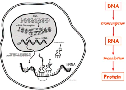
This section aims to give an overview of the gene regulation process within a living cell. The genome of an individual is defined as the hereditary infor-mation encoded in its genetic material. Therefore, it contains all inforinfor-mation needed by the organism to develop and live. The physical support of the genome is a molecule called DesoxyriboNucleic Acid (DNA). The general aspect and localisation of DNA is illustrated on figure 1.1.

A single DNA strand is a sequence of nucleotides, which are composed of a phosphate group, a sugar and a base. There are four types of bases which are thymine (T), adenine (A), guanine (G) and cytosine (C). Then, a double DNA strand is made of two single DNA strands which form complementary bonds in the following way : a T base is always complementary with an A and a G base is complementary with a C. This double strand of complementary base pairs has the shape of an helix. It is coiled around proteins called histones and then super-coiled to form a chromosome, which is located in the nucleus of the cell. In humans, there are 23 pairs of chromosomes.

All cells in an organism contain the totality of the genome, that is to say,

2 CHAPTER 1. CONTEXT

Figure 1.1: General aspect and localisation of DNA in a eukaryotic cell

the whole DNA sequence. The central dogma of biology (cf figure 1.2) states that coding genes on DNA are transcribed into messenger RNA (mRNA) that transport themselves outside the nucleus, to be translated into proteins. Each protein has a specific function to achieve inside the cell. Some have cellular functions: they might serve for cell motility, for maintaining the cell structure, for communication with the outside, for transporting molecules... Some proteins, called enzymes have a biochemical function, meaning that they serve as catalyzers to chemical reactions. In a word, proteins are the main actors of a cell’s activity.

However, the cells of an organism are not all the same. Their activity, and therefore the type and quantity of proteins they produce, varies according to their location and to the environmental conditions they are facing. For instance, a liver cell and a blood cell do not behave identically. Likewise,

1.1. BIOLOGICAL CONTEXT 3

Figure 1.2: The central dogma of biology

variations in the environment like a change of temperature or the presence of some chemical compounds, do result in an adaptive behaviour of a cell. As a consequence, a cell does not express all coding parts of the genome, in the sense that there are genes that do no result into functional proteins into that cell. This also means that a cell is able to modulate the production of its proteins to satisfy its needs. This process is called gene regulation. There are several levels of gene expression regulation:

• DNA level regulation

In order to allow for transcription, the structure of DNA must be mod-ified. Some enzymes are responsible for DNA methylation or histone modifications that strengthen DNA packing, thus preventing the tran-scription machinery from accessing the sequence to be transcribed. • Transcriptional regulation

Among the proteins produced by a cell, some are called transcription factors (TF) and their function is precisely to regulate gene expression. A single TF has a certain number of gene targets. RNA polymerase is an enzyme complex responsible for transcription initiation. It binds to particular DNA sequences named promoters. By recognizing a target’s binding site, a transcription factor increases (or decreases) the affinity of RNA polymerase for that gene’s promoter, thus allowing (or disabling) its transcription into mRNA. In the first case, the TF is an activator,

4 CHAPTER 1. CONTEXT

whereas it is called an inhibitor in the second case. Figure 1.3 gives an example case of the activating regulation of gene A on gene B. In condition 1, gene A is transcripted and translated into an activator TF protein, which binds to the operator (O) of gene B, allowing RNA polymerase to bind the promoter (P), which initiates transcription of gene B into mRNA, which is then translated into a triangular protein. Then, under a second condition, which could be an external stimulus or that it has been produced in a sufficient quantity, the triangular protein is not needed anymore. The TF becomes inactive (see the change of shape), it cannot bind anymore to the operator, RNA polymerase is not recruited and transcription does not happen.

• Post-transcriptional regulation

Being transcribed is a necessary but not sufficient step for being trans-lated into a functional protein. Between transcription and translation, the transcripts undergo various processing mechanisms. They are sta-bilized (capping and polyadenylating) and spliced. Splicing is a mecha-nism that removes introns (non-coding regions). But, they can also be sequestated and degradated. At this stage, gene silencing and degra-dation are processes which participate to a regulation system named RNA interference whose main actors are micro RNAs (miRNA) and small interfering RNAs (siRNA).

• Translational regulation

At last, translation itself can be disabled mainly at the beginning of the translation by the ribosome.

In this thesis, we focus on the particular case of transcriptional regulation. In particular, we neglect the last two types of regulation and assume that measuring mRNA quantities is sufficient to measure gene expression.

1.1.1.2 Why study gene regulation?

Elucidating the regulatory structure of a cell is a long-studied issue to which many efforts have been devoted. If we were able to understand a cell’s func-tional mechanisms, we could predict its behaviour under different stimuli, like for instance the response to a drug. Another practical application in biomedicine is the search for new therapeutic targets. Trying to cure some disease, one often wishes to be able to inhibit or enhance some particular functional pathway. For instance, one could imagine a novel cancer ther-apy which would stop cancerous cells from proliferating while not being too toxic for surrounding tissues. As another example, Plasmodium falciparum

1.1. BIOLOGICAL CONTEXT 5 !"#$%&"#'(' )*+,-.&#+'+*#*' /' 1' 0' )*+,-.2*$'+*#*' 3' 4"-5)6/' 27.#897%4&"#' :)6/' 27.#8-.&"#' .9&;.2"7'<=' 27.#897%4&"#' :)6/' 27.#8-.&"#' 17"2*%#' !"#$%&"#'(' )*+,-.&#+'+*#*' /' 1' 0' )*+,-.2*$'+*#*' 3' 24.#564%7&"#' 8)9/' 24.#5-.&"#' .6&:.2"4';<' 9"' 24.#564%7&"#' =>2*4#.-'5&8,-,5?'"4'*#",+@'74"2*%#' ?'"4'%2'%5'#"2'#**$*$'.#A8"4*' 7"-A)9/'

6 CHAPTER 1. CONTEXT

is a parasite responsible for malaria. Some strains of this parasite are now resistant to known treatments. Unraveling the defense mechanisms of this parasite could allow to disable them and to design a new efficient treatment.

1.1.1.3 Experimental characterization

Low-throughput assays Historically, the first attempts to discover tran-scriptional regulatory interactions were carried out by experimental biolo-gists. A regulatory interaction is, as we have described above, a binding reaction between a protein (the transcription factor) and a DNA fragment (the target gene’s binding site). We review here the main experimental tech-niques used for assessing protein-DNA interactions.

• Gel shift analysis

A DNA fragment, marked with a fluorescent marker is put on a gel, which has previously been impregnated with a protein. Since binding slows down the fragment, the difference in speed at which the DNA fragment moves along the gel with and without a protein, indicates whether the protein and DNA bind.

• DNase footprinting

This technique exploits the fact that a protein binding to a DNA frag-ment tends to protect this fragfrag-ment from cleavage. A DNA fragfrag-ment of interest is amplified and labeled at one end. The obtained fragments are separated in two portions. The first portion is incubated with the protein of interest and DNase, a DNA cleaving enzyme. The second portion is incubated with DNase but without the protein of interest. The amount of DNase is calibrated so that each fragment is cut once. Both samples are then separated by gel electrophoresis1 and the cleav-age pattern in the presence of the protein is compared to the pattern in the absence of the protein.

• Nitrocellulose filter binding assay

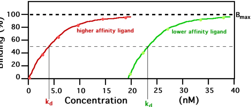
This assay aims to estimate the strength of interaction between a pro-tein ligand and a DNA fragment by measuring the binding constant as a function of the protein quantity. Nitrocellusose paper, used as a filter, is ideal for immobilizing proteins, whereas DNA will not stick to it unless being bound to a protein. Radioactively labeled DNA is incubated with a known amount of protein and the mixture is spilled

1_{A technique for separating molecules placed on a gel matrix, by subjecting them to} the action of an electric field.

1.1. BIOLOGICAL CONTEXT 7

on a nitrocellulose filter, placed above a vacuum which pumps the liq-uid downward. This way, all DNA which is not bound to a protein is removed. Then, radioactivity is measured, reflecting the quantity of bound DNA. This is repeated for various amounts of protein, so that we obtain a function plot of the amount of bound DNA against the amount of protein. A rapidly increasing curve shows a high affinity (cf figure 1.4).

Figure 1.4: Results of a filter binding assay.

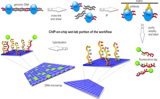
High throughput technologies A major drawback of the methods pre-sented so far is their cost in terms of time and money. Indeed, one has to replicate manually the experiment for each pair of protein-DNA fragment one wants to test. That is why high-throughput experimental assays have been designed, which allow to test for many pairs at the same time. Here we focus on the ChIP-on-chip technology, also know as genome-wide local-ization analysis. The ChIP-on-chip technique, which stands for Chromatin ImmunoPrecipitation on chip, is a widely used technique for testing DNA-protein interactions. More specifically, such an experiment aims to identify the binding sites of a DNA-binding protein, such as a transcription factor. Figure 1.5 illustrates the experiment which we roughly describe. The protein is linked to the DNA in an in vivo environment. Then, DNA is chunked and the protein is targeted with a specific antibody, which allows to retrieve complexes made of a protein and a DNA fragment bound to it (a step called chromatin immuno-precipitation). These fragments are separated from the protein of interest and they are spotted on a DNA microarray (a chip)2 _in

8 CHAPTER 1. CONTEXT

order to identify them. The ChIP-Seq technology is the same, except that the identification of the fragments is made by sequencing and mapping them on a reference genome. It is more sensitive than ChIP-on-chip and less prone to saturation effects of the signal.

Figure 1.5: The ChIP-on-chip experiment.

1.1.1.4 In silico inference

Switching to the systems biology paradigm Even though high through-put assays have alleviated the experimental burden, a ChIP-on-chip exper-iment is still restricted to a single TF protein. Moreover, results still lack reliability. For instance, there are interactions which remain difficult to char-acterize by a ChIP-on-chip assay because it is not possible to design an antibody to recognize the protein of interest, or because an antibody exists but is not specific enough to this protein. In a general perspective, the great complexity of cellular mechanisms, generated by the numerous interactions existing in the cell between genes or proteins, makes it a grueling (and expen-sive) work to elucidate biological networks in situ i.e through experimental means. For those reasons, whether they are reliability or cost issues, in silico (computational) methods are increasingly appealed to for the inference of regulatory interactions.

1.1. BIOLOGICAL CONTEXT 9

The problem of regulatory interaction inference as we have depicted it, typically fits into the scheme of systems biology. We have already pointed out that cells could have very complex behaviors. Classical biology studies these behaviors by dissecting the cell and zooming on a few of its compo-nents. In opposition to that point of view, systems biology claims that one cannot understand the way a cell functions unless one sees it as a system, where any biological function is the result of thousands of components inter-acting, rather than the product of the activity of some isolated components. The two main problems that have caught the attention of systems biologists are network inference and model validation. In the context of transcriptional regulation, network inference consists in the elucidation of regulatory inter-actions between the components of the cell. This task is often referred to as “reverse engineering” in literature. The model validation part deals with the search for some general design principles underlying the regulatory struc-tures. Fitting a model to an inferred network structure, we are allowed to make predictions which in turn, help to gain insight on the mechanistic of the cell . A common way to proceed is to reduce the complex machinery to a more simple model, whose parameters and/or shape allow one to test some hypotheses. Then, the model is usually validated by carrying out simulations. While reverse engineering operates at a very global scale, model validation often necessitates to focus on smaller networks, first because fitting a model on a too large network is difficult and also for interpretation purposes (some particular pathways of interest can be studied more precisely).

It is worth noting at this stage that the goal of systems biology is not to discard experimental biology. Both approaches are meant to complement each other in an iterative scheme. Whenever a computational algorithm is trained to infer an interaction network, high confidence interactions need to be experimentally validated. Likewise, whenever a model is found to be plausible, it needs to be checked by experimental means. In any case, the objective of computational methods is to guide experimentalists who would otherwise have to move blind. In turn, it is important that systems biologists can rely on the biologists’ experience and knowledge, to build meaningful and relevant models. A crucial remark we can make about network inference is that, in this iterative scheme, it seems important to produce some confidence score for each interaction, so that only the most likely TF/gene pairs are submitted to experimental validation. In other words, it seems that the job expected from computational methods is above all a prioritization job.

10 CHAPTER 1. CONTEXT

Learning the edges between the nodes Under the systems biology vi-sion, it is convenient to view the regulatory machinery as a graph. Naturally, the nodes of the graph are be genes, proteins or any acting component one wants to study and an edge represents an interaction between two of these components. Figure 1.6 gives a representation example of a regulatory net-work. In this particular example, nodes are heterogeneous and edges are directed. Red nodes are genes coding for transcription factor proteins (which we can directly call transcription factor as well) and blue nodes are other non-TF coding genes. A directed edge can only be drawn from a red node, meaning that the corresponding TF regulates the expression of the corre-sponding target gene.

Figure 1.6: A graph representation of a regulatory network.

Having represented the transcriptional machinery as a graph, the task of is equivalently stated as “learning the edges between the nodes of the graph”. A common way to proceed is to start from the output of a network, namely the expression levels of genes in order to get back to what has generated these expression patterns, that is the original structure of the network. DNA microarrays are devices that provide expression level measures (see section 4.5). A gene is featured by an expression profile that describes the activity of that gene under various conditions (steady state data) or at various time points (time-series data). We now give a brief review of methods which infer regulatory networks de novo from gene expression data. Mainly, these meth-ods differ in the interpretation of the graph representation. We detail below the mathematical formalism they use, their specificities and the assumptions they make.

• Clustering methods [Eisen et al., 1998, Amato et al., 2006]

1.1. BIOLOGICAL CONTEXT 11

indicating co-expression. Indeed, co-expressed genes are likely to par-ticipate to the same pathways and therefore, to be functionally related. Therefore, an edge between two genes on the graph is not directed and cannot be interpreted as a regulatory interaction but rather as a functional relationship. Steady-state as well as time-series data can be used.

• Correlation-based and information-theoretic methods [Butte and Ko-hane, 2000, Margolin et al., 2006, Faith et al., 2007]

The rationale behind these approaches is that an interaction between a TF-coding gene and one of its targets can be detected through the de-pendence relationship that is induced between their expression levels. Information-theoretic methods use the mutual information measure, which can be seen as a measure of departure from independence. Con-trary to correlation-based methods, information-theoretic methods are able to detect more complex forms of dependence than just linear de-pendence. An undirected edge between two nodes on the graph stands for a (linear) dependency between the expression of the two genes. If correlation is used, one can distinguish between activating and inhibit-ing regulation, accordinhibit-ing to the sign of correlation. However, causality cannot be determined through correlation only and therefore, an edge might just represent an indirect regulation. To avoid this, the concept of partial correlation has been proposed, which computes correlation between two variables conditional to all other variables [Rice et al., 2005, Liang and Wang, 2008].

• Boolean network inference [Akutsu et al., 2000]

In that particular setting, the expression level of a gene i is encoded as a Boolean variable Xi: Xi = 1 means “expressed” as opposed to a value

of 0. To do so, expression profiles are discretized into binary vectors. The value of the Boolean variable Xi depends on the values of the

nodes pointing to it through a logical function. We note that this type of inference produces qualitative rather than quantitative relationships. The logical function for one node can vary over time or not, depending on which type of data is used.

• Bayesian network inference Friedman et al. [2000], Beal et al. [2005], Yu et al. [2004b]

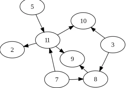
A graphical model represents conditional independence relationships of a set of random variables by means of a graph. A Bayesian network is a particular type of graphical model where the graph is a directed acyclic graph. Figure 1.7 gives an example of such a graph. Each

12 CHAPTER 1. CONTEXT

variable is represented by a node and each node is independent to all other nodes conditionally to its parents. For instance, figure 1.7 shows that conditionally to variables 5 and 7, variable 11 is independent from variables 2, 3, 8 , 9 and 10. Given the conditional dependency graph

Figure 1.7: A directed acyclic graph.

G, data D and a model for the conditional likelihood (gaussian for instance), one can compute the posterior probability of that graph given the data D and maximize it with respect to G. In practice, since this optimization is an NP-hard problem, Bayesian inference methods resort to heuristic searches of the optimal graph. Bayesian networks have been extended to dynamic bayesian networks which additionally take into account the evolution over time of the regulatory network.

• Ordinary differential equations (ODE) methods [Gardner et al., 2003, di Bernardo et al., 2005, Bansal et al., 2006]

While previous methods consider mainly statistical dependencies be-tween the nodes, ODE-based methods are deterministic by nature and they focus on causal relationships. Following the principles of chemical kinetics, the expression variation of each gene is related to the level expression of all other genes and possibly to an external signal via a differential equation. The parameters of that equation are estimated by fitting the data to the model. These parameters determine the nature of the edges. A basic example is when the variation of the expression

1.1. BIOLOGICAL CONTEXT 13

of a gene xj is chosen to be linearly related to the expression level of

other genes_{xi}i�=j ˙ xj = � i�=j ai∗ xi

Coefficients ai are computed to fit the data and they are interpreted

as weights on edges leaving from xj to the x�is. In essence, ODE-based

methods are well suited for the analysis of time-series data, but they can also be used with steady-state expression profiles, in which case

˙

xj = 0 ∀j.

In silico methods are meant to investigate a very wide search space. To handle the level of complexity one is faced with when adopting a systemic point of view, one has to resort to simplifying assumptions. Linearity or dis-crete node value are examples of simplifying assumptions. We see that the approaches we have presented above adopt different formalisms correspond-ing to different assumptions on the data and on the way interactions might be captured. Some take into account the nature of the interactions (is the TF an activator or an inhibitor) while others do not, some do consider their dynamics (different interactions may be active at different time points). At last, some, like ODE-based methods, are able to infer synergistic effects while others are not. Besides, the complexity of the networks to be learnt might raise underdetermination issues, meaning that the available data might be insufficient to determine a single solution. To overcome this issue, one can also encode prior beliefs in the algorithm in order to restrict the search space and to guide the inference process. These priors beliefs often come as evolu-tionary constraints [Marbach et al., 2009] and are used to guide the inference towards biologically plausible networks. For instance, many computational methods enforce some sparsity constraints on the network structure and claim that gene networks tend to be parsimonious for the robustness property this confers them [Leclerc, 2008]. A possible way to proceed is to restrict the in-degree of the nodes [Akutsu et al., 2000]. Indeed, it is a widely accepted fact that each gene is regulated by a small set of regulators. This is related to the scale-free property which states that the networks we want to infer con-tain a few densely connected nodes called “hubs”, while the rest of the nodes have very few connections. Moreover, studying the topology of some known regulatory networks, it has been noticed that some particular motifs would appear more frequently than what would be expected by chance. Again, this feature can be used to enforce the algorithm to output realistic networks.

14 CHAPTER 1. CONTEXT

1.1.2

The disease gene hunting problem

In this section, we introduce the problem of disease gene hunting. Then, we briefly review the traditional approaches that were used to identify disease genes.

1.1.2.1 Disease gene discovery

Having discovered the path which leads from genes to proteins and therefore to a corresponding phenotype, the task of finding which genes are respon-sible for the appearance of a given phenotype has attracted great attention in the genetic scientists community. In particular, a burning topic during the past 20 years has been to identify those genes whose disruption lead to acquired Mendelian diseases. Mendelian diseases are genetically inher-ited diseases caused by a mutation in a single gene. They are sometimes called monogenic diseases. For instance, cystic fibrosis (or mucoviscidosis) is a Mendelian disease caused by a mutation in the gene for the protein cystic fibrosis transmembrane conductance regulator (CFTR). The Online Mendelian Inheritance in Men (OMIM) database [McKusick, 2007] was ini-tially created to gather knowledge on Mendelian disease/gene associations. However, efforts have been progressively shifting to the harder task of finding genes associated with polygenic or complex diseases. Indeed, the disruption of a single gene is sometimes not enough to trigger a disease phenotype, and it is thought that instead, the disease is caused by the simultaneous action of several genes and possibly by environmental factors. Yet, the mode of action of this set of genes is unknown and if environmental factors are playing a role in the development of the disease, it is uneasy to distinguish the environ-mental basis from the genetic causes. Alzheimer’s disease is an example of a complex disease. The main reason why researchers concentrate their efforts on the disease gene hunting is that many diseases remain misunderstood. The identification of novel causal genes would give additional insight on the mechanisms which are at the origin of these poorly known diseases and above all, could open the way for the design of new therapies to cure them.

1.1.2.2 Experimental approaches for disease gene identification Traditional strategies for finding disease genes are mixed strategies involving both molecular biology and genetic (statistical) techniques. There are mainly three ways to proceed.

Candidate gene approach This approach requires prior knowledge of the diseases, such as the type of function that is perturbed by the disease or the

1.1. BIOLOGICAL CONTEXT 15

tissues that are affected [Kwon and Goate, 2000]. Candidate genes are pri-oritized using his knowledge and then tested in association studies. These studies gather a set of individuals, some of whom are affected by the dis-ease, some of whom are healthy people. The candidate gene is statistically tested for segregating polymorphisms among this population of individuals. Namely, if a given allele of that gene is significantly inherited more frequently in subjects having the disease than in healthy subjects, it is acknowledged as a disease gene. We can make a distinction here between population-based studies and family-based studies. Population-based studies allow the inclu-sion of any subject in the population and is similar to a classical epidemiology study. Genotypes are looked for that are more present in the case population than in the control population of healthy subjects. The inclusion plan of such a study must be made carefully, since the genotype frequency also varies be-tween subjects of different geographical and/or ethnic origin. Otherwise, the success of the study might be hampered by what is called a stratification con-founding effect. On the other hand, in family-based studies, healthy parents are used as controls for their affected offspring. They avoid the confounding stratification effect but since members from the same family live in the same environmental conditions, the role played by the candidate gene is not clearly separated from that of environmental hidden factors. A general drawback of the candidate gene approach is that it might fail if the disease pathophysiol-ogy is currently misunderstood or our knowledge of it is incomplete, which is often the case.

Genome-wise Association Studies Single Nucleotide Polymorphisms are variations on a single base pair of the genome between individuals of the same species. They represent around 90% of human genetic variations. SNP arrays are a special type of DNA microarrays (see section 4.5) which are designed to detect such polymorphisms on the whole genome for a given population. They have marked the advent of genome-wise association stud-ies(GWAS). GWAS are association studies such as described in the previous paragraph except they examine systematically all SNPs across the genome. They are different from candidate gene studies because they do not use any knowledge of the disease to focus on particular genes but rather proceed to extensive statistical tests for association between a phenotype and genomic variations.

Genomic screen approach Contrary to the previous approach, genomic screening is a systematic method which operates without any prior knowl-edge on the studied disease. It relies on the use of “genetic markers” and

16 CHAPTER 1. CONTEXT

“genetic linkage”. Genetic markers are highly polymorphic3 _{DNA sequences}

(possibly genes) whose location on the genome is known. They are evenly distributed on the genome and usually serve as identifiers of the genome (like kilometer markers on a road). Genomic linkage could be defined as an inher-itance property. During meiosis, DNA segments are exchanged between the chromosome inherited from the father and that inherited from the mother. This process, called recombination, allows to create new trait combinations and participates to genetic diversity. The consequence of that crossing-over is that alleles that would have been inherited together otherwise, can now be split up in different daughter cells. Moreover, it has been observed that the chances of being split-up by a recombination event were higher for alle-les further away from each other. Therefore, if a marker is observed to be frequently inherited along with the phenotype of interest, this indicates that the gene responsible for that phenotype is likely to be close to it. The genetic distance between two markers is defined as the recombination frequency, i.e the proportion of recombining meiosis. A recombination frequency of 1% corresponds to a genetic map unit and is called a centiMorgan (cM). The corresponding physical distance (in number of bases) varies according to the localization on the genome. There are statistical tests which allow to identify two markers delimiting a candidate region, likely to contain the responsible gene. Figure 1.8 is extracted from [Silver, 1995] and illustrates the whole pro-cess: in this example, the phenotype of interest is “green eyes”. Two markers D3Ab34 and D3Ab29 are found to have a recombination frequency with the phenotype of 2 over 400, one marker, D3Xy12, had a frequency of 1 over 400 and D3Xy55 was concordant in all 400 cases (panel A). Therefore, the candidate region was delimited by markers D3Ab34 and D3Ab29 (panel B). Then, fine mapping of this region can then be achieved by a technique called positional cloning. This comprises a time consuming procedure called chro-mosome walking, which consists in moving forward from the first delimiting marker towards the second, getting each time closer to the gene of interest. The process is aided by hybridizing a series of overlapping clones from a li-brary to the region. The ordered series of such clones is called a contig, which can be seen as a physical representation of the region. These clones are easily identifiable. At each step of the walk, specific tests (including co-segregation tests) can determine whether the current clone belongs to the gene that is looked for. In panel E of figure 1.8, we see the results of co-segregating tests for the different clones. 1R and 10R show one recombining event (resp. in individuals number 156 and 332), while 6L and 2R fragments are concordant

3_{A gene is said to be polymorphic if it comes into different shapes or “alleles” in a} population, yielding different versions of the same phenotype.

1.1. BIOLOGICAL CONTEXT 17

with the phenotype. Therefore, localization of the “green eyes” locus is en-hanced and restricted to a narrower region between 1R and 10R. Although the initial interval is narrowed down, the output of positional cloning is usu-ally not a gene but rather an interval, whose size depends on the resolution limit (on the order of 1-10 cM). Candidate genes in that interval must then be examined successively. Note that the evolution of sequencing technologies now allows to save a lot of times. Nevertheless, both approaches necessitate recruiting a large number of families and collecting DNA samples from the members of these families, which is still a very long and heavy process.

Prioritization using in silico methods Considering the inherent diffi-culty of traditional techniques of disease gene identification, and the fact that researchers were often left with a remaining list of thousands of genes to in-vestigate, there were a growing need for automated techniques. That is why this area of research has turned towards computer scientists and mathemati-cians to develop computational techniques. Similarly to the gene regulation case, what is expected from in silico methods in the case of disease gene discovery is rather a prioritization job than a classification job. That is to say the desired output of an algorithm is an ordered list of genes, where the top genes are believed to be the better disease gene candidates.

1.1.3

Data resources

The increasing need for automated methods is a general phenomenon in bi-ology, that goes far beyond the two particular problems presented in this thesis. It is true that for many biological problems, experimental techniques are time consuming and sometimes very expensive but this fact by itself is insufficient to explain the growing success of computational biology nor why mathematicians, statisticians and computer scientists have got interested in the biological issues. This phenomenon takes a lot more sense if we place under the light of what can be termed a “data revolution”. This revolution has been triggered by the completion of the Human Genome Project in 2003. The goal of this project was to determine the sequence of base pairs which constitute human DNA and to identify all human genes. This achievement was a considerable step towards understanding molecular mechanisms in gen-eral and was chosen to mark the advent of the post-genomic era. Since then, biotechnologies have evolved at a fast pace and advances in that field have generated an unprecedented variety of data, describing living cells at a very high precision level. Among them, high-throughput techniques have enabled researchers, for the first time in history, to characterize biological samples through a high number of quantitative measures at the genome scale. As a

18 CHAPTER 1. CONTEXT

1.1. BIOLOGICAL CONTEXT 19

practical consequence, data analysis and mathematical/statistical modeling have been increasingly integrated at the core of biological research. Besides, the analysis of datasets having the size and complexity of those produced by high-throughput technologies raise challenging methodological issues that require appropriate statistical treatment.

In the two problems we have introduced earlier, the principal object to be described is a gene. Therefore, we now review the different types of data that are now available to characterize genes or equivalently the proteins they code for. Figure 1.10 illustrates further a few types of data that are available to describe a gene and gives a better idea of the kind of quantitative information they provide.

1.1.3.1 Transcriptomics data

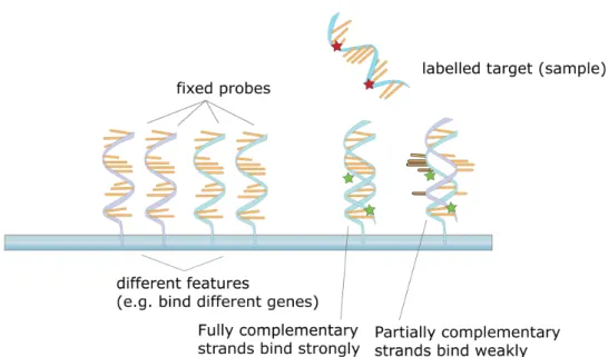
The most well known type of high-throughput data to describe genes is proba-bly transcriptomics data, also known as microarray expression data. Microar-rays are devices for measuring the level of expression of all genes in a tissue in a particular condition or time point. The expression level of a gene is quan-tified via the abundance of messenger RNA after transcription of that gene. We mentioned in section 1.1.1 that this was a simplification, since measuring the quantity of proteins would be more sensible to quantify expression. The corresponding data are called proteomics data. However, proteomics tech-niques are far less mature than transcriptomics and researchers implicitely consider that transcriptome is correlated enough with proteome to provide a good approximation of the actual expression of a gene. For a broad expla-nation of the technical details, a microarray is a solid suppport, also called a “chip”, with an arrayed series of spots, each of which contains a fixed amount of probes. A probe is a short sequence designed to match a specific mRNA. The target sample is fluorescently labeled and hybridized to the probes on the array. A labeled mRNA matching a probe generates a light signal whose intensity ideally depends on its quantity (see figure 1.9). The intensity signal is captured (see left picture on figure 1.10) and processed to yield a single quantitative measure for each gene. Affymetrix and Agilent are two compa-nies whose microarray technology is widely spread in the genomic research community. Finally, a single microarray produces a snapshot of the activity of a tissue sample in a particular condition. Generally, this process is re-peated in different conditions (steady-state data) or at different time points (time series data). Different conditions usually means either different samples (from normal individuals versus patients with a disease, or different tissues) or different environmental conditions (oxydative stress, drug, temperature

20 CHAPTER 1. CONTEXT

change, PH change...). Time series experiments may be designed to observe how expression evolves in time after a given event (for instance, knock out of a gene or subjecting the sample to a drug). In both cases, one eventually obtains an expression profile or each gene which is a vector of measures that characterizes the gene in question.

Figure 1.9: Target samples are hybridized to probes on a microarray.

A related type of expression data, which is perhaps less popular, is Ex-pressed Sequence Tag (EST) data. EST are short sequenced fragments of complementary DNA (cDNA) obtained from mRNA bits sampled from a given tissue. These fragments are indicators of expression of a gene. There-fore, they can be used to identify yet unknown genes by physical mapping. But even when the corresponding gene is already known, the information about the tissues and the conditions in which the gene was found to ex-pressed is still valuable and can be used to describe this gene. For instance, in the candidate approach for disease gene discovery we have been reviewing previously, if one was looking for a gene responsible for a disease affecting the brain, she would start by investigating those genes known to be expressed in this area of the body.

1.1. BIOLOGICAL CONTEXT 21

1.1.3.2 Subcellular localization data

An important feature for a gene is the localization within the cell of the pro-tein it codes for. Knowing where a propro-tein lives enables one to know more about its function, about it interacting partners. It can also be a valuable information for who would like to target this protein. Laboratory techniques encompass immuno-fluorescence, fluorescent microscopy, fractionation com-bined with mass spectometry.

1.1.3.3 Sequence data

The sequencing technologies are probably those that have known the most spectacular development since their invention in the late seventies (they were independently discovered by Sanger’s team in the UK and Maxam and Gilbert’s team in the US). Nowadays, it has become straightforward to char-acterize a gene by its nucleotide sequence. A lot of work has been dedicated to sequence analysis, sequence alignment and sequence comparison. Sequence analysis has allowed to identify particular structures, recurrent patterns or motifs associated with specific types of sequences. An important application of sequence alignment and comparison has been to find homologous proteins. Homologous proteins are coded by genes deriving from a common ancestor. Going a step further, one can distinguish between two types of homologous proteins:

• Paralogous proteins belong to a single species and result from a dupli-cation event.

• After a speciation event, the two copies of the same gene in the two newly formed species are brought to evolve separately and therefore their sequence and possibly function diverge. They are called ortholo-gous.

However, even after billions of years, homologous genes might have kept a certain degree of resemblance, both because their sequences are similar and because their function might be conserved. Homology is often detected by means of sequence similarity. Detection of homologous proteins is the ground of comparative genomics. or instance, when looking for the function of a gene (protein), a fruitful approach is to look for informations from similar proteins either in other better known species, via its orthologous proteins or possibly within the same species, via its paralogous proteins.

22 CHAPTER 1. CONTEXT

Data available

Biologists have collected a lot of data about proteins. e.g.,

Gene expression measurements

Phylogenetic profiles

Location of proteins/enzymes in the cell

How to use this information “intelligently” to find a good function that

predicts edges between nodes

.

Jean-Philippe Vert (ParisTech) Inference of biological networks 6 / 37

Data available

Biologists have collected a lot of data about proteins. e.g.,

Gene expression measurements

Phylogenetic profiles

Location of proteins/enzymes in the cell

How to use this information “intelligently” to find a good function that

predicts edges between nodes

.

Jean-Philippe Vert (ParisTech) Inference of biological networks 6 / 37

!""#####!"$####%####!"&# !_$"#####!_$$####%####!_$&# # #######%### !'"#####!'$####%####!'&# ()')#"# ()')#$# #%# ()')#'# !"#$%!!!!!!&'()!!!!!!* !!!!)+!,-! ()')#"# ()')#$# #%# ()')#'# * #######"#####%######*# " #######*#####%######*# # ########%### * #######*#####%######*# !./$01!!!!2/#3!!!!!!*!!!!!&4%! !""#####!"$####%####!"&# !$"#####!$$####%####!$&# # #######%### !'"#####!'$####%####!'&# ()')#"# ()')#$# #%# ()')#'# !"#$%!!!!!!&'()!!!!!!* !!!!)+!,-! ()')#"# ()')#$# #%# ()')#'# * #######"#####%######*# " #######*#####%######*# # ########%### * #######*#####%######*# !./$01!!!!2/#3!!!!!!*!!!!!&4%! !"#"$%$ !"#"$&$ $'$ !"#"$#$ !"#$%&#'!!!()%*+!!!,!!-&./012&! ( $$$$$$$($$$$$'$$$$$$%$ % $$$$$$$%$$$$$'$$$$$$%$ $ $$$$$$$$'$$$ % $$$$$$$($$$$$'$$$$$$($

Expression data Phylogenetic data Cellular localization data Figure 1.10: Different data representation for genes.

1.1.3.4 Annotation data

Annotation is a generic term that refers to the process of attaching biological knowledge to a gene or a protein. This biological knowledge covers many types of information. Here is a non-exhaustive list.

Phylogenetic profiling Phylogenetic data are typically produced by com-parative genomics methods. For each gene A in a given species (let’s say a human gene) one can look for orthologous genes in a list of other species (for instance, mouse, worm and pig). As mentioned above, this is done by measuring sequence similarity. BLAST (Basic Local Alignment Tool) is a popular tool to output such measures [Altschul et al., 1990]. By threshold-ing the BLAST score, one can get a binary vector of size 3 (the number of other species) with 1 indicating that your gene has an orthologous gene in the corresponding species. Comparing genes using such phylogenetic profiles makes sense since it is believed that genes conserved in the same species are likely to be functionally related.

Functional annotation Functional annotation is meant to describe what is known about the function of a gene. For instance, Gene Ontology (GO)

1.1. BIOLOGICAL CONTEXT 23

database [Ashburner et al., 2000] structures this information via a controlled vocabulary of terms, embedded into a hierarchical tree. For instance, the term “intracellular organelle” has for parent term “intracellular part” and for children “cytoplasmic vesicle”. The list of GO terms associated with a gene describes that gene at the functional level. Besides molecular functions per-formed, these terms can describe biological processes (or pathways) in which the gene is involved and cellular components in which it is active. Simi-larly, a gene can be attached a list of pathways it participates to. Pathway membership can be found for instance in the Kyoto Encyclopedia of Genes and Genome (KEGG) database [Kanehisa et al., 2004]. KEGG works fol-lowing the same type of organization. As an example, pathway hsa05218 is named “Melanoma-Homo sapiens” and belongs to the class of “Human diseases;cancers”. Both types of data can presented as binary matrix (like localization or phylogenetic data, see figure 1.10), each column correspond-ing to a GO or KEGG term. Likewise, literature contains vast amounts of biological information, which be be automatically searched with text mining tools, like TXTGate [Glenisson et al., 2004].

Functional relatedness is even more directly reported in physical interac-tion data (Protein-protein interacinterac-tion or PPI), which we therefore meninterac-tion here, even though they are not exactly annotation data. PPI data can be found in numerous databases, such as Bind, Biogrid, Dip, Human Protein Reference Database (HPRD), IntNetDb, IntAct or String [Bader et al., 2003, Stark et al., 2006, Xenarios et al., 2002, Mishra et al., 2006, Xia et al., 2006, Aranda et al., 2010, Jensen et al., 2009].

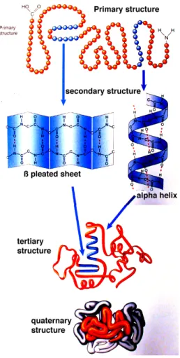
Structural annotation When translated from a messenger RNA, a pro-tein is folded so as to acquire a particular structure, this is illustrated in figure 1.11. As can be seen on this picture, the structure of a protein is really difficult to describe. At the level of the primary structure, the de-scription concerns the sequence of amino-acids. Sequence analysis can also be performed directly at the gene level. As briefly mentioned, it deals with identifying motifs that are recurrent patterns in the chain of amino-acids (or nucleotides). Examining co-occurrence of identical motifs in two gene se-quences is a possible way to compare them. At a higher level, there are parts of the protein that can evolve independently from the rest of the chain. They are called domains and they are widely used to annotate proteins. The pres-ence of common domains in two proteins is a clue for functional relatedness. InterPro is an example of a database which might contain such information on a protein.

24 CHAPTER 1. CONTEXT

1.2. MACHINE LEARNING CONTEXT 25

1.1.3.5 Data fusion

As a conclusion of this long and yet incomplete list of data types, there are many ways to characterize a gene. Each data representation has its own specificities and all of them carry very different information with respect to the problem at hand. As a result, it is highly probable that the results one can obtain from a single data type are incomplete but complementary to those obtained with different views. Besides, it is likely that the relationship between different data contain some information as well. To get the whole picture, a natural idea is therefore to incorporate many data sources in the inference process. This is currently referred to as data fusion. There are many ways to proceed. One that is quite straightforward is to combine the results obtained from different data sources a posteriori. For instance, in the context of regulatory network inference, you could learn a first set of edges {Eexpr} using gene expression data, a second set {Ephylo} using phylogenetic

data and take as a final result either the union or intersection of these two sets of edges. Intuitively, taking the intersection reduces the set of predicted edges, hence drastically decreasing sensitivity, all the more so as the sets have a small overlap. For that matter, it is a known issue that inference methods often lack robustness and that data perturbation results in weakly overlap-ping predictions. In that case, taking the union tends to hinder precision. Furthermore, this solution does not fit in a prioritization perspective, since it cannot handle properly ranked lists of predictions. A second option is to integrate the data sources a priori, i.e to find a way to combine them first and to give this as input to the learning process to finally output a ranked list of predictions. We subsequently indicate a way to do this in section 1.2.

1.2

Machine learning context

We have already stressed the need for automatized methods to tackle com-plex biological problems. Among scientific disciplines, machine learning is particularly well adapted to that framework. It can be defined as a sub-domain of artificial intelligence which designs algorithmic techniques aimed at giving a machine the ability to learn. It deals with the automatic extrac-tion of informaextrac-tion from input data, aided by computaextrac-tional and statistical methods. Examples of topics that typically appeal to machine learning are natural language processing, computer vision, written digit recognition, robot locomotion or video games. In this thesis, we show that they can be partic-ularly useful in biology. This section is dedicated to a brief introduction to the main machine learning tools we have used, that are kernel methods and

26 CHAPTER 1. CONTEXT

more specifically Support Vector Machines (SVM).

1.2.1

Learning from data

In a very general context, machine learning algorithms need to be fueled with data in order to produce an output. To formalize this, consider that data are actually a collection of objects or individuals, each described by p random variables or “features”. We denote by X = (X1, . . . , Xp) these features. We

assume that their distribution is unknown and that, however, we want to learn something from these features.

1.2.1.1 Unsupervised versus supervised learning

A major distinction can be made regarding the kind of information one wants to retrieve. If one wants to learn anything about the data distribution itself, he will perform “unsupervised learning”. This includes density estimation or learning about the topographical organization of the distribution (via clus-tering or manifold inference, for instance). The learner will be aided by a training set which consists in observations of the p variables (actual measure-ments of these variables) for n objects or individuals:

xi ∈ Rp, i∈ (1, . . . , n)

On the other hand, if the output is some other variable Y = (Y1, . . . , Yn), we

are dealing with “supervised” learning. In this case, the inference is guided and the goal is to guess the relationship between the input variable X and the output variable Y, under the shape of a generic function which links them: Y = f (X). This time, as a training set, the learner is given a vector of values of Y for the n objects: [yi]i∈(1...n) in addition to the matrix of measurements

[xi]. A typical strategy is to define a loss function that quantifies the cost of

incorrectly predicting the output. Then, the algorithm’s objective will be to minimize the expectation of that loss. Since this expectation is unknown, the theoretical objective criterion will be estimated by an empirical criterion. If we denote the loss function by L, the algorithm boils down to the following optimization problem ˆ f = argmin f n � i=1 L�f (xi), yi) � . (1.1)

1.2.1.2 The bias-variance trade-off

To start with, the function f is generally searched for in some determined Hilbert function space _{H. A major challenge is to determine how complex}