Modification of semantically enriched FE mesh models

HAL Id: pastel-00608202

https://pastel.archives-ouvertes.fr/pastel-00608202

HAL is a multi-disciplinary open access

archive for the deposit and dissemination of sci-entific research documents, whether they are pub-lished or not. The documents may come from teaching and research institutions in France or

L’archive ouverte pluridisciplinaire HAL, est destinée au dépôt et à la diffusion de documents scientifiques de niveau recherche, publiés ou non, émanant des établissements d’enseignement et de recherche français ou étrangers, des laboratoires

Ruding Lou

To cite this version:

Ruding Lou. Modification of semantically enriched FE mesh models. Computer Aided Engineering. Arts et Métiers ParisTech, 2011. English. �NNT : 2010ENAM0017�. �pastel-00608202�

Università!degli!Studi di!Genova! !! 2010"ENAM"0017! ! ! ! ! ! ! ! ! ! ! ! ! !

presented and defended publicly by

Ruding LOU

June 21st, 2011

Modification of semantically enriched FE mesh models

Application to the fast prototyping of alternative solutions in the context of industrial maintenance_!

PhD T H E S I S

to obtain the degrees of

Docteur délivré par

l’École Nationale Supérieure d'Arts et Métiers

Spécialité “Conception”

École doctorale n°432 : Sciences des Métiers de l'Ingénieur

and

Dottore di Ricerca

dell' Università degli Studi di Genova

in “Ingegneria Meccanica” della Scuola

in Scienze e Tecnologie Innovative per l'Ingegneria Industriale (XXIII ciclo)

Directors of thesis: Philippe VÉRONandBianca FALCIDIENO Supervisors: Jean-Philippe PERNOTandFranca GIANNINI

T

H

E

S

I

Mme. Dominique BECHMANN,Professor, Université de Strasbourg Reviewer

Mme. Stefanie HAHMANN,Professor, INP-Grenoble President

M. Umberto CUGINI,Professor, Politecnico di Milano Reviewer M. Rinaldo C. MICHELINI,Professor, Università degli Studi di Genova Fonction

M. Philippe VÉRON,Professor, Arts et Métiers ParisTech PhD co-supervisor M. Jean-Philippe PERNOT,Associate Professor, Arts et Métiers ParisTech PhD co-supervisor Mme. Franca GIANNINI,Senior Researcher, CNR-IMATI.Ge PhD co-supervisor M. Alexei MIKCHEVITCH,PhD Engineer, EDF Division R&D Guest

It is a pleasure to acknowledge and thank several persons who helped me both during my PhD study and in the evaluation of the thesis. My sincere thanks go to my thesis directors Dr. Philippe VERON, Professor of Arts & M´etiers ParisTech (France) and Dr. Bianca FALCIDIENO, Director of the National Research Council (Italy) for their guidance and support.

Next, I express my deepest recognition to my thesis co-supervisor in France, Associate Professor Jean-Philippe PERNOT. He brought me into the world of computer graphics research and made me interested in this topic. Thanks to him, I have gained advanced knowledge in this field of research and also in some associated fields of fundamental science.

I appreciate the care of my thesis co-supervisor in Italy, Senior Re-searcher Franca GIANNINI, both for the scientific quality of her guid-ance and for the kind reception she gave me during my first stay in Italy.

Further, I thank the members of the jury, professors Dominique BECHMANN, Stefanie HAHMANN, Umberto CUGINI and Rinaldo C. MICHELINI, for their careful evaluation of my thesis.

Thanks also go to Dr. Alexei MIKCHEVITCH and Rapha¨el MARC, who were my advisors at EDF, the industrial partner of my PhD study. They helped me discover and appreciate the engineering efforts of the

I further thank my ex-colleague Dr. Minica PANCHETTI, who helped me with mesh modelling during her PhD thesis. Thanks also go to Aur´elien BARGIER, former engineer student at Arts & M´etiers ParisTech and Sai-Jing PENG, current PhD student at Beihang Uni-versity, who made significant contributions to my PhD study during their internships. I also thank all the members in the lab. LSIS in France and all my colleagues at IMATI—also for their friendly recep-tion during my research work in Italy.

Last, but not least, I thank my parents Guoying LOU and Ren´e ANDRON, who have taken care on me and pushed me to go fur-ther in my studies in France, and my fianc´ee Lirong XI for her love and care during 10 years—and forever.

Behaviour analysis is largely performed on the virtual model of the product before its physical manufacturing. The move from the reality to the digital world is gainful since it avoids the high costs in terms of money and time spent on intermediate manufacturing required for performing simulations on real products. Anyhow, the process could be further optimised especially during the product behaviour optimi-sation phase. This process involves repetition of four main processing steps: CAD design and preparing for meshing, mesh creation, en-richment of the model with physical semantics and Finite Element Analysis (FEA). The product behaviour analysis is performed on the first design solution as well as on the numerous successive product optimisation loops. Each design solution evaluation necessitates the same time as required for the first product design and it is particularly crucial in the context of maintenance and lifecycle assessment. This thesis proposes a new framework for CAD-less product optimi-sation through FEA which reduces the mesh preparation and FEA semantics enrichment activities. More concretely, the idea is to di-rectly operate on the firstly created FE mesh, enriched with phys-ical/geometric semantics, to perform the product modifications re-quired to achieve its optimised version.

In order to accomplish the proposed CAD-less FE analysis framework, modification operators acting on both the mesh and the associated semantics need to be devised. In this thesis, the underlying concepts and the devised components for the development of such operators are discussed. A high-level operator specification is proposed according to a modular structure that allows an easy realisation of different mesh modification operators. Finally, four instances of this high-level

L’analyse de comportement est largement utilis´ee sur les mod`eles virtuels de produits avant ses fabrications physiques. Le passage de la r´ealit´e vers monde num´erique est gagnant parce-que cela ´evite les cots ´elev´es en termes de temps et d’argent consacr´ees `a la fabrication in-term´ediaires n´ecessaires pour r´ealiser des simulations sur des produits r´eels. Quoi qu’il en soit, le processus pourrait encore ˆetre optimis´e en particulier pendant la phase d’optimisation du comportement de produit. Ce processus implique la r´ep´etition de quatre principales ´etapes de traitement : conception et pr´eparation pour mailler de la CAO, cr´eation de maillage, enrichissement de s´emantique physique sur le mod`ele et calcul ´el´ement finis (EF). L’analyse de comporte-ment de produit est effectu´ee sur la premi`ere solution de conception ainsi que sur les nombreuses boucles successives d’optimisation de produit. Chaque ´evaluation de solution n´ecessite le mˆeme volume de temps que celui n´ecessaire pour la premi`ere conception de produit, cela est particuli`erement crucial dans le contexte de maintenance et d’´evaluation de cycle de vie de produit.

Cette th`ese propose un nouveau cadre de travail pour l’optimisation de produit sans CAO via au calcul EF, qui r´eduit les activit´es de la pr´eparation de maillages et de l’enrichissement de s´emantiques cal-cul EF. Plus concr`etement, l’id´ee est d’exploiter directement sur le maillage EF premi`ere fois cr´e´e qui est enrichi par des s´emantiques physiques et g´eom´etriques, en vue d’effectuer les modifications n´ecessaire de produit pour atteindre ses versions optimis´ees.

Pour r´ealiser le cadre de travail propos´e pour le calcul EF sans CAO, les op´erateurs de modifications agissant `a la fois sur les maillages et sur

de ces op´erateurs sont discut´ees. Une sp´ecification d’op´erateur de haut niveau est propos´ee selon une structure modulaire qui permet une r´ealisation facile des diff´erents op´erateurs de modification de maillage. Enfin, quatre instances de cet op´erateur de haut niveau sont d´ecrites: la fusion, la fissuration, le per¸cage et le cong´e d’arˆete. Ces op´erateurs sont prototyp´es et valid´es sur les mod`eles EF acad´emiques et indus-triels, ce qui montre clairement la faisabilit´e de notre approche.

L’analisi del comportamento `e ampiamente usato su modelli virtuali di fisica realizzazione dei suoi prodotti prima. Il passaggio della realt`a al mondo digitale `e un vincitore, perch´e evita gli elevati costi in termini di tempo e denaro speso per beni strumentali necessari per eseguire simulazioni su prodotti reali. In ogni caso, il processo potrebbe essere ottimizzato in particolare durante la fase di ottimizzazione del com-portamento del prodotto. Questo processo comporta la ripetizione di quattro fasi principali di lavorazione: progettazione e preparazione di CAD a maglia, la creazione della maglia, l’arricchimento semantico del modello fisico e di calcolo ad elementi finiti (FE). L’analisi del comportamento del prodotto, si procede sulla soluzione primo pro-getto cos come molti successivi cicli di ottimizzazione del prodotto. Ogni valutazione di soluzione richiede la stessa quantit`a di tempo di quello richiesto per la progettazione del prodotto in primo luogo, ci`o `e particolarmente cruciale nel contesto della manutenzione e della va-lutazione del ciclo di vita del prodotto.

Questa tesi propone un nuovo quadro per l’ottimizzazione del prodotto senza l’utilizzo di CAD per calcolare EF, che riduce l’attivit`a di prepa-razionedi griglie e arricchimento del computing EF semantica. Pi`u concretamente, l’idea `e di operare direttamente sulla maglia EF prima creato, che si arricchisce di semantica fisiche e geometriche, di ap-portare le modifiche necessarie per raggiungere i suoi versioni del prodotto ottimizzato.

Per realizzare il quadro proposto per il calcolo EF senza operatori CAD modifiche agendo su entrambe le griglie e la semantica asso-ciata deve essere considerato. In questa tesi, i concetti di base e

ulare che permette una facile implementazione di differenti operatori modifica della maglia. Infine, quattro istanze di questo livello opera-tore sono descritti: la fusione, rottura, perforazione e lasciare il bordo. Questi operatori sono prototipi e validato i modelli FE nelle univer-sit`a e nell’industria, che dimostra chiaramente la fattibilit`a del nostro approccio.

Abstract iv

R´esum´e vi

Astratto viii

Contents x

List of Figures xvi

Introduction 1

PART I Hight-level manipulations of Finite Elements meshes :

state-of-the-art 4

1 Models, methods and tools for industrial studies 5

1.1 Geometric models along the product lifecycle . . . 6

1.1.1 Early representation schemes . . . 6

1.1.2 Decomposition schema . . . 9

1.1.3 Constructive Solid Geometry (CSG) . . . 10

1.1.4 Boundary representation (B-Rep) . . . 11

1.1.5 Sweep representation . . . 14

1.1.6 Implicit and Parametric representations . . . 14

1.1.6.1 Implicit method . . . 15

1.1.6.2 Parametric method . . . 15

1.1.8 Subdivision surfaces . . . 17

1.1.9 Synthesis on the use of geometric models along the PLC . 19 1.2 Basic mesh techniques . . . 19

1.2.1 Mesh generation . . . 19

1.2.2 Mesh simplification and refinement . . . 22

1.2.2.1 Simplification . . . 22

1.2.2.2 Refinement . . . 25

1.3 Numerical simulation based on FEA for product design, optimisa-tion and maintenance studies . . . 28

1.3.1 Classical CAD-FEA loop . . . 30

1.3.2 Industrial case studies using classical CAD-FEA loop . . . 31

1.3.3 Notion of groups and type of FEA semantics . . . 35

1.3.4 Model modification operation categories . . . 39

1.3.5 Specificities in some industrial simulation contexts (main-tenance, Reverse Engineering · · ·) . . . 41

1.3.5.1 Lake of time in the re-creation of specific meshes 42 1.3.6 Absence of the CAD model (starting from scratch) . . . . 42

1.3.7 Tuned meshes . . . 43

1.3.8 What would be a possible solution generally speaking ? . . 44

1.4 Conclusion . . . 46

2 Modification of enriched FE meshes 48 2.1 Criteria for FE mesh modification methods . . . 48

2.1.1 Geometric criteria . . . 49

2.1.2 Semantic criteria . . . 50

2.1.3 Categorisation of mesh modification methods to be studied 51 2.2 Mesh intersection . . . 52

2.3 Crack feature / contact zone insertion . . . 59

2.4 Cutting operation . . . 61

2.5 Mesh filleting . . . 64

2.6 Semantics manipulations . . . 66

PART II CAD-less modelling operators 69

3 Generic CAD-less approach for fast preparing of FE meshes 70

3.1 Multi-layered framework . . . 70

3.1.1 Geometry level or mesh modification . . . 73

3.1.2 Group or geometric semantic Level modification . . . 75

3.1.3 Simulation semantic level modification . . . 79

3.1.3.1 Model Shape Semantics . . . 79

3.1.3.2 Finite Element Analysis (FEA) Semantics . . . . 80

3.1.3.3 Shape of group . . . 81

3.2 Components of the CAD-less geometric modelling operator . . . . 82

3.3 Information exploitation . . . 83

3.4 Geometric modification stage . . . 83

3.5 Simulation semantics transfer stage . . . 85

4 Basic methods and tools for the geometric treatment of enriched FE meshes 86 4.1 Shape recogniser . . . 87

4.1.1 Categorisation of basic shapes . . . 87

4.1.2 Technique to identify planar area . . . 88

4.1.2.1 The normal vector method based on one triangle 89 4.1.2.2 The planar equation method based on one triangle 89 4.1.2.3 The best fitting plane with a set of triangles (adopted solution) . . . 93

4.1.3 Techniques to identify spherical areas . . . 95

4.1.4 Technique to identify cylindrical areas . . . 100

4.1.5 Freeform . . . 104

4.1.6 Overall algorithm and examples . . . 104

4.2 Sharp feature recognition . . . 110

4.2.1 Sharpness weight on an edge . . . 111

4.2.2 Discrete curvature on a node . . . 114

4.2.3 Use of sharp feature detection in CAD-less mesh modelling operator . . . 119

4.3 Mesh quality checking . . . 121

4.3.1 Aspect ratio of elements . . . 121

4.3.2 Self-intersection . . . 122

4.4 Topological operations . . . 122

4.4.1 Triangulation in edge loop . . . 122

4.4.2 Tetrahedralisation in closed triangle surface . . . 126

4.4.3 Duplication . . . 127

4.5 Mesh deformation . . . 130

4.5.1 The adopted mechanical model . . . 132

4.5.2 Force Density Method formalisation . . . 134

4.5.3 Optimisation problem formulation . . . 137

4.5.4 Shape constraint formalisation . . . 139

4.5.5 Different minimisations . . . 140

4.5.6 New shape constraints for CAD-less mesh modelling operator143 4.6 Conclusion . . . 147

5 Basic models, methods and tools to handle semantics 148 5.1 Basic characteristics of mesh groups . . . 149

5.1.1 FE mesh group dimension classification . . . 149

5.1.2 Topology of mesh groups . . . 150

5.1.3 Relationships between mesh groups . . . 151

5.2 Middle-level semantics transfer . . . 153

5.2.1 Preservation of group boundary . . . 154

5.2.2 Concepts of Virtual Group Boundary (VGB) . . . 155

5.2.2.1 VGB of groups defined over a 2D mesh . . . 156

5.2.2.2 VGB of groups defined over a 3D mesh . . . 157

5.2.3 Preservation of group content . . . 159

5.2.4 Decomposition into Elementary Groups (EG) . . . 161

5.3 High-level semantics transfer . . . 167

5.3.1 Proposal of high-level semantics classification . . . 167

5.3.2 Towards rules for high-level semantics transfer . . . 170

6 A generic CAD-less mesh modelling operator and its

instantia-tions 180

6.1 Structure of the operator (recall) . . . 181

6.2 Mesh merging operator . . . 182

6.2.1 Overview of the enriched meshes merging process . . . 183

6.2.2 Intersection computation . . . 185

6.2.2.1 Contact faces detection . . . 187

6.2.2.2 Intersection curves definition . . . 188

6.2.2.3 Intersection curve optimisation . . . 189

6.2.3 Intersection zone re-meshing . . . 191

6.2.3.1 Re-meshing zone definition . . . 192

6.2.3.2 Re-meshing zone cleaning . . . 194

6.2.3.3 Filling holes and updating the semantics . . . 196

6.2.4 Experimentation results . . . 198

6.2.5 Mesh merging in face/face mode . . . 202

6.3 Mesh cracking operator . . . 203

6.3.1 Overall process of planar crack insertion into semantically enriched meshes . . . 205

6.3.2 Mesh element classification and Crack Interface identification208 6.3.3 Crack Interface pre-treatment . . . 209

6.3.4 Crack Interface deformation . . . 215

6.3.5 Additional examples . . . 219

6.4 Mesh drilling operator . . . 222

6.4.1 Mesh elements classification . . . 224

6.4.2 Interface identification and pretreatment . . . 226

6.4.3 Constraint definition and deformation . . . 231

6.4.4 Additional examples . . . 235

6.5 Mesh filleting operator . . . 239

6.5.1 Overview of the mesh filleting process . . . 239

6.5.2 Definition of sharp edges to be filleted . . . 240

6.5.3 Filleting area definition . . . 243

6.5.4 Surface filleting zone deformation . . . 246

6.5.6 Additional experimentations with the mesh filleting operator248

6.6 Conclusion . . . 253

Synthesis, conclusions and perspectives 255

Limits and shortcomings of actual engineering . . . 256

Challenge of faster, easier and accurate modelling approach . . . 257

Perspectives . . . 259

A Synth`ese longue en fran¸cais 262

1.1 Wireframe model representation and possible solids can be deduced

from it . . . 7

1.2 Parameterised primitive instancing schema examples . . . 8

1.3 A 2D object represented by 2D spatial decomposition . . . 10

1.4 CSG in 3D modelling . . . 11

1.5 A Boundary Representation used for object modelling and corre-sponding graph . . . 12

1.6 Non-manifold B-Rep modelling of an object . . . 13

1.7 Sweep a section along a guide . . . 14

1.8 Examples of surface mesh (a) filled in completely (b) or partially (c) 17 1.9 Multi-resolution subdivision surfaces [126] . . . 18

1.10 Quad-tree decomposition of a simple 2D object . . . 20

1.11 Example of advancing front on a simple 2D object . . . 21

1.12 (left) Example of Delaunay criterion maintains the criterion while (right) does not . . . 21

1.13 Mesh simplification and mesh refinement . . . 23

1.14 Local simplicial complex transformations [46] . . . 24

1.15 Illustration of the “TetFuse” operation [23] . . . 24

1.16 Longest-Side Bisection of triangle t0 [95] . . . 27

1.17 8-subtetrahedra subdivision [92] . . . 27

1.18 Example of 4 steps simulation loop (a,b,c,d) to introduce and anal-yse possible local structural modifications of a caisson (e,f,g) (cour-tesy EDF R&D) . . . 33

1.19 Numerical assessment of a new solution based on the classical prod-uct optimisation method: stiffener addition to a U-like testing bench model (courtesy EDF R&D) . . . 34

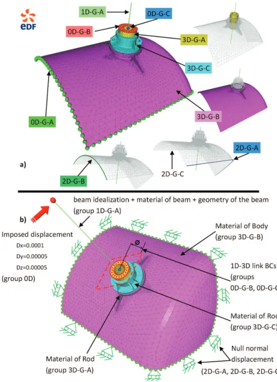
1.20 Groups and associated FEA semantics defined on the CAISSON (courtesy EDF R&D) . . . 36

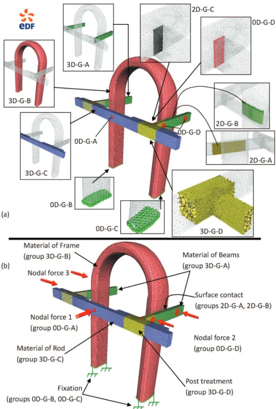
1.21 Groups and associated FEA semantics defined on the U-like testing bench (courtesy EDF R&D) . . . 38

1.22 Example of inner / outer corner filleting . . . 40

1.23 Crack insertion into the mesh model in order to model a crack phenomenon (courtesy EDF R&D) . . . 41

1.24 Workflow for FE mesh model preparation (courtesy EDF R&D) . 45

1.25 Example of stiffener addition onto a Caisson model (courtesy EDF R&D) . . . 46

2.1 Approximate Boolean operations on free-form triangle meshes [15] 52

2.2 Approximate boolean operations on large polyhedral solids with partial mesh reconstruction [122] . . . 53

2.3 Hybrid Booleans [87] . . . 54

2.4 Intersecting and trimming parametric meshes on Finite-Element shells[28] . . . 56

2.5 Mesh offsetting and intersection repairing [54] . . . 56

2.6 Surface triangulation over intersecting geometries [105] . . . 57

2.7 Contact interface re-meshing in context of assembly collision de-tection [24] . . . 58

2.8 Merging of intersecting triangulations for finite element modeling [22] . . . 59

2.9 Automatic crack-insertion for arbitrary crack growth [18] . . . 60

2.10 Supporting cuts and FE deformation in interactive surgery simu-lation [83] . . . 61

2.11 Simulating Drilling on tetrahedral meshes [117] . . . 62

2.12 Interactive TIN modification with a cutting tool [31] . . . 63

2.14 Offset triangular mesh using the multiple normal vectors of a vertex

[55] . . . 65

3.1 Different layers information of an enriched FE model . . . 71

3.2 Considered geometric modifications at the lowest level of the frame-work . . . 74

3.3 Examples of geometric modifications with (b) and without (c) group preservation . . . 76

3.4 Shape semantics changes derived by geometry modification . . . . 80

3.5 FEA semantics changes according to geometry modification . . . . 81

3.6 FEA semantics changes according to geometry modification . . . . 82

3.7 Component-based of the CAD-less mesh modelling approach . . . 84

4.1 Plane detection using normal comparison . . . 91

4.2 Plane equation computation based on one or several reference tri-angles . . . 93

4.3 Selection of the reference faces with tolerable normal variation . . 94

4.4 Selection of reference faces from one face (R0_{) and its first} neigh-bours (R1_{) . . . . 98}

4.5 Example of shape detection without triangle minimum number control . . . 107

4.6 Basic shapes recognition examples . . . 110

4.7 Sharp feature examples [45] . . . 111

4.8 Sharp feature examples [45] . . . 112

4.9 Top view of a mesh with the concerned edge e and the parameter plane used for the BFP method [48] . . . 113

4.10 Angle between the two polynomials used for the ABBFP method (side view) [48] . . . 114

4.11 (a) Geometric parameters of a star-set associated to a node p; (b) edge length and dihedral angle β [60] . . . 114

4.12 (a,b,c) the same geometry at node p is described by equivalent meshes, (d) circular sectors associated to the star-set of the node p [60] . . . 117

4.14 Hierarchical triangulation . . . 125

4.15 (a) Triangle mesh with a hole; (b) triangulation by minimising the area; (c) triangulation by maximising the aspect ratio . . . 126

4.16 Example of tetrahedral mesh generated from a surface mesh by Tetgen [106] . . . 127

4.17 Duplications of 2D mesh elements . . . 129

4.18 Different utilities of mesh deformation (a, b) mesh relaxation; (c, d) curvature preservation on patches junction; (e, f) circle shape rendering from zigzag shape . . . 131

4.19 Network of springs associated to geometric model . . . 133

4.20 Repositioning of nodes on a mesh (a, b) and on a mesh with FDM (force density method) . . . 134

4.21 Example of bar network . . . 135

4.22 Nodal displacement definitions (c, d), displacement of pure mesh (a, b) and displacement of mesh coupled with a FDM mechanical model (e, f) . . . 139

4.23 minimisation of external forces only applied on the free nodes (a), minimisation of external forces applied on the free and blocked nodes (b), minimisation of external force variation on free nodes (c) and minimisation of external forces variation on free and blocked nodes (d) [90]. . . 142

4.24 Example of deformation using force minimisation under plane and cylinder type constraint . . . 145

4.25 Mesh deformation for rendering a sphere shape by iterative min-imisation . . . 146

5.1 Different topologies of group: (a) simply connected (b, c) con-nected with holes and (d) disconcon-nected . . . 151

5.2 Different relative spatial relationships between two groups . . . . 152

5.3 Example of group definition preservation during the mesh merging 154

5.4 Examples of VGBs extracted from groups defined over a 2D trian-gle mesh . . . 157

5.6 Definition of EGs from two partially overlapping groups of nodes and faces . . . 165

5.7 EGs computation on a triangular mesh model of the caisson (cour-tesy EDF R&D) . . . 166

5.8 Geometric modification around groups . . . 172

5.9 Example high-level semantics transfer . . . 173

5.10 Examples of possible high-level semantics transfer . . . 175

5.11 Examples of possible high-level semantics transfer . . . 176

6.1 Component-based of the CAD-less mesh modelling approach (fig.3.7

on page 84) . . . 181

6.2 Two contact modes between two triangle meshes: (a) face/edge, (b) face/face . . . 182

6.3 Overview on the merging algorithm for two enriched meshes . . . 184

6.4 Workflow and necessary tools for merging meshes . . . 186

6.5 Contact faces detection using Bounding Box intersection . . . 187

6.6 Intersection curve construction . . . 188

6.7 Intersection curve construction . . . 189

6.8 Intersection branch optimisation according to the ℓaaverage length

criterion, the nodes n1 and n6 are considered as particular nodes . 190

6.9 Two intersection meshes with different density (a), Re-meshing of intersection faces (b) and re-meshing of intersection faces plus their neighbourhood of different bandwidths (c) . . . 192

6.10 Subdividing two elementary holes A and B (a) into four elementary holes (b) . . . 196

6.11 Comparison between the minimum area (a) and the maximum as-pect ratio (b) triangulation criteria . . . 197

6.12 Merging of two scanned models (a, courtesy of MPII), two spheres intersecting smoothly (b) and an example of non-manifold config-uration (c). . . 200

6.13 Overall merging approach on the example of two stiffeners that have to be merged with a caisson model. (courtesy EDF R&D) . . 201

6.14 Two scanned stones merged using an approach similar to the face/edge mode . . . 203

6.15 CAD-less mesh crack operation schema . . . 204

6.16 Workflow and necessary tools for the crack operator . . . 205

6.17 Rough crack interface computation over a 3D mesh containing three groups . . . 207

6.18 Rough crack interface identification . . . 209

6.19 Examples of problem on the interface in 2D mesh . . . 211

6.20 Examples of tetrahedra associating with 2, 3,or 4 crack interface triangles (upper) and their corresponding deformed versions (lower)212

6.21 Examples of problem on the interface . . . 213

6.22 Splitting schema for the tetrahedron with 2 potential interface tri-angles . . . 214

6.23 Constrained deformation for insertion of a planar crack into the 3D mesh containing 3 groups . . . 215

6.24 Crack operator applied on a cube-like tetrahedral mesh having 3 groups . . . 220

6.25 Crack operator applied on a sphere-like tetrahedral mesh having 6 groups . . . 221

6.26 Insertion of a crack into a 3D mesh model (courtesy EDF-R&D) . 222

6.27 CAD-less mesh drilling operation schema . . . 223

6.28 Workflow and necessary tools for mesh drilling operator . . . 225

6.29 Mesh elements classification . . . 226

6.30 Two kept triangles associating with 2 or 3 drilling interface edges (a, b) and the corresponding deformed version (c) . . . 227

6.31 Examples of a kept tetrahedron associating with 2 drilling interface triangles (a) and with 3 drilling interface triangles (c) and their corresponding deformed versions (b, d) . . . 229

6.32 Drilling interface updating for case of kept triangle associating with 2 interface edges . . . 231

6.33 Rough hole generation (a,c) and mesh deformation (b,d) . . . 235

6.34 Creation of a through hole in a 3D mesh while preserving the shapes of the groups . . . 236

6.35 Multiple drills on the Stanford Bunny characterized by four groups of tetrahedra having spherical VGBs . . . 237

6.36 Insertion of a cylindrical hole into the 3D mesh of a caisson model (courtesy EDF-R&D) . . . 238

6.37 Workflow and necessary tools for the mesh filleting operator . . . 241

6.38 Relative sharp edges searching process stops in 3 cases . . . 242

6.39 Different filleted areas based on various range numbers (from 1 to 4)245

6.40 Two-steps deformation for tetrahedral mesh filleting . . . 247

6.41 Example of tetrahedral mesh filleting . . . 249

6.42 CAD-less filleting on a tetrahedral mesh . . . 250

6.43 Tetrahedral mesh filleting of a hook . . . 251

6.44 Example of tetrahedral mesh filleting on a half-piston . . . 252

A.1 Boucle classique dans l’´etude num´erique sur le comportement de produits (courtoisie EDF-R&D) . . . 263

A.2 Diff´erentes solutions d’optimisation du mod`ele CAISSON(courtoisie EDF-R&D) . . . 266

A.3 Trois niveaux d’information port´ee par un maillage EF . . . 269

The Finite Element Analysis (FEA) plays a key role for evaluating the multiple solutions in the context of product design and maintenance. This is due to the fact that FEA helps to reduce the time development and/or maintenance times while saving money. It reduces material costs by testing for safety and behaviour with less material or alternative materials and it reduces physical prototyping costs by proving and improving the product design before it is produced. It avoids long-time physical prototyping of the various envisaged product optimisa-tion soluoptimisa-tions. All these advantages are very valuable for competitive engineering and maintenance purposes. Since FEA is widely used in numerous industrial companies, it is crucial to think whether the FEA workflow can be optimized and improved to save additional time as well as money. Nowadays, the mainstream methodology for product behaviour analysis and conceptual solution assessment using FEA relies on the following steps: 1) Computer-Aided Design (CAD) modelling, meshing and preparing the CAD model for specific meshing, 2) Finite Element (FE) mesh meshing, 3) Physical semantics modelling, 4) Finite Element simulation and result analysis. These four stages constitute the loop for a product design solution evaluation. According to the obtained results of the FE simula-tion, experts may start another optimisation loop for another design solution or improve the FE modelling; we refer to this process cycling as optimisation loop. Each optimisation loop for each product design solution necessitates repeating all the above listed four stages from CAD until simulation.

However, in the context of current maintenance and lifecycle problem analy-sis, the product already exists, the CAD models are not necessarily available and the product behaviour has to be studied and improved during its exploitation. Companies exploiting industrial complex installations are currently submitted to

various constraints crucial from a production point of view. They can be relative to the time and cost of the production process stops, to the efficiency of main-tenance solutions, to production safety criteria, etc. For example, in the field of power production, it is critical to identify the problem source and to provide the appropriate solution while taking care of the triplet: Time, Quality and Cost. As a reference, the total cost of one day of stop of a nuclear power station repre-sents several hundreds of thousands of Euros. In the context of power production equipment maintenance, it seems quite clear that the reduction of the time of the projects carried out by engineering departments (fast operational study, solution optimisation for maintenance) may lead to important research perspectives in terms of fast numerical prototyping and solution assessment methods during the operational study. This reduction concerns the time spent notably for various numerical simulations (e.g. mechanical resistance assessment, vibration analysis, lifecycle contra-expertise). We found that for each optimisation loop we spend a lot of time on preparing the FEA model: 1) The CAD modelling necessitates modifying the previous CAD model or creating completely a new one if it is not available; 2) the mesh modelling stage needs to make the CAD model meshable and to specify different characteristics on the mesh: different sizes of mesh ele-ments, non-manifold meshing, (i.e. double mesh entities, disjoint entities, · · ·), etc.; 3) to simplify defining different physical semantics on the mesh model, dif-ferent groups of mesh elements should be created before. The first result of simulation allows tuning/certifying the model, in case of failure it is necessary to come back to the CAD/meshing/FE model creation stages for modifying the simulation model. In the context of product maintenance, the structural optimi-sation modification concerns locally around the problem zone. For saving time the interesting way for fast evaluating the solution by FEA is to directly prototype the modification on the existing FEA mesh model previously validated.

In this thesis, the definition of a new prototyping method has been investi-gated: the proposed CAD-less fast prototyping approach avoids going back to the CAD models during the fast numerical solution assessment. Actually, the idea is to enable direct modification of complex meshes enriched with semantics for fast and accurate FE simulation of production installation behaviour during the operational studies. This approach should avoid multiple and time-consuming

iterative updating of the CAD models, as well as the tedious re-meshing steps of potentially complex shapes. Not only the newly defined modification operators have to take into account multiple geometric aspects and constraints, but they also have to consider semantic data associated to the FE meshes: groups of FE entities must be maintained during various mesh modifications. The FE groups can contain nodes, edges, faces and 3D elements (tetrahedra, hexahedrons, etc.) or the mix of different topology FE elements. These semantic data enrich the FE mesh models with information that are classically relative to the diverse parame-ters of geometric and mechanical nature (materials, FE modelling type, boundary conditions, external loads, etc.) required for FEA. The proposed approach is par-ticularly efficient in the case of fast prototyping of local structural modifications on a given production installation since it does not worth to redo the entire FEA semantics enriched mesh for making locally small modifications. It can also be applied during the product preliminary design phases where many alternative solutions often have to be tested and simulated. This thesis is organised in two parts. The first part introduces the models, methods and tools classically adapted for FE Analysis (chapter 1) and details the way enriched meshes can be modified using today’s’ available tools (chapter2). In the second part, the proposed CAD-less approach is presented. Chapter3 describes the aspects of a model that have to be taken into account in the generic approach. The basic methods and tools for modifying the meshed geometry are introduced in the chapter 4 whereas the basic methods for manipulating semantics in a mesh are presented in the chapter

5. Finally, the chapter 6describes how a generic CAD-less operator is built from newly introduced basic methods and tools. It also details different instances of such a operator. The last chapter ends the manuscript while concluding and opening perspectives to this work.

of Finite Elements meshes :

state-of-the-art

In the first part, the general context of this PhD thesis is introduced. The context includes scientific and industrial background. This thesis is located in the domain of product design and maintenance studies aided by computer threfore different product design approaches are presented at first. Then the industrial engineering context is shown as well as some concret industrial examples in maintenance based on EDF’s (´Electricit´e De France) needs are given. The typical problem from industrial point of view today is that the model preparing for FEA is very heavy in the sense that for FE model improvement as well as new design product assessing the classical FEA loop should be repeated.

In order to speed up the FEA model preparation process, this thesis proposes to manipulate directly the FE semanticlly enriched meshes without going back to the CAD model. Therefore a full state of art on manipulations of FEA meshes are then analysised. Various criteria are listed in order to analyse whether the research works could response the industry needs.

At the end, we propose our method allowing modifying directly the FE se-mantics enriched meshes taking into account different industrial constraints as mesh quality, FE group presence, etc.

Models, methods and tools for

industrial studies

Computer-Aided Engineering (CAE) is wildly spread in the world along with the development of computer science. CAE is the broad usage of computer software to assist in engineering tasks along the product life cycle (PLC). This includes Aided Design (CAD), Aided Analysis (CAA), Computer-Integrated Manufacturing (CIM), Computer-Aided Manufacturing (CAM), Ma-terial Requirements Planning (MRP), and Computer-Aided Planning (CAP). Along these different phases the physical solid to be studied is represented by a numerical geometric model.

Today in most industries Computer-Aided Engineering is normal practice. Production is driven by Computer-Aided Design, Analysis, and Manufacturing. All the data relative to the product development process are stored and managed by Product Data Management (PDM) systems which may contain all the models used at different steps. For processing a so-called Digital Mock-Up (DMU) various tools and methods are mandatory. In the first part of this chapter, an overview of the most used methods for geometric modelling are presented. In the second part, the manipulation of the DMU is introduced and notably the techniques relative to the adaptation of the DMU for FEA, which is the core of the thesis. Different industrial highlighted problems are illustrated from examples in maintenance numerical studies of power production equipment.

1.1

Geometric models along the product

lifecy-cle

The geometric modelling concerns the methods and algorithms for describing and manipulating digital shapes [2, 93]. A model is a mathematical abstraction of a physical object or phenomenon and has to be converted into a representation to be computationally treated. In product development, geometric models are created during the design phases for describing the shapes of the product at the beginning of the PLC development using CAD tools. Then, according to the various needs (simulation, manufacturing, etc.) different models are needed. Generally, the geometric modelling consists in creation, exchange, visualisation, animation, interrogation, and annotation of digital models of physical objects. Different approaches of geometric modelling are presented in the following sub-sections.

1.1.1

Early representation schemes

Different early model representations are presented in [2]. Approaches of geo-metric modelling have begun before the rise of computers and with pencil and paper. Since the advent of computers, the approaches of geometric modelling have changed a lot. Engineering drawings were the earliest attempts to model objects. Computers were not involved and they were intended as a means of communication among humans. The engineering drawing often had errors but humans were able to use common sense to end up with correct result. There was no formal definition of such drawings as a representation scheme. The basic idea was to represent objects by a collection of planar projections.

Wireframe representations were the first representation schemes adopted for three-dimensional linear polyhedrons in computer-aided tools. It is a natural ap-proach, the idea being to represent objects using only their edges. But wireframe representations are ambiguous, the well-known example that consists of 16 ver-tices and 32 edges is shown in figure 1.1.a. It represents a solid and each of the quadrilaterals (some of them are squares) defines a face of the solid. The inner cube can represent a hole but it is not defined the direction of the opening of the

cube. Therefore, it could be one of the three possibilities (fig.1.1.c - fig.1.1.d) for this opening. Some works have been done for identifying the solid from wire-frame models [119,120].

Figure 1.1: Wireframe model representation and possible solids can be deduced from it

Many early commercial modelling systems have used wireframe representa-tions. However, wireframe models are ambiguous and are not anymore used for representing the object in today’s applications but for visualisation purposes. Many systems support a wireframe display mode because it is efficient (i.e. only vertices and edges are displayed and processed). For example, wireframe visu-alisation can be used for preview purpose. Rendering a complex model or an animation sequence could be very time-consuming if all objects have to be ren-dered. If wireframe models (usually including its face information) are available, one can easily obtain a general feeling of the final result without waiting for minutes or even hours before spotting a design flaw. The edges in a wireframe model do not have necessarily to be line segments. They can be curve segments and in this case the edge table will be more complicated since in addition to the two endpoints a description of the joining curve segment (e.g. an equation) is required.

Faceted representation is a simple solution which circumvents the major limits of the wireframe representation by adding faces. This representation is am-biguous in collision detection for the case where two objects are intersecting and their faceted representations are not intersecting. There is a difference between a modelling system using a faceted representation and one using a faceted display.

The second one means that objects are displayed by linear polyhedra even though the system may maintain an exact analytic representation of objects internally.

Parameterised primitive instancing [93] scheme is based on the notion of families of objects, each member of a family being distinguishable from the other by few parameters. Every scheme has primitives, which must be instantiated to construct structured representations. Primitives may be low level, e.g. the points used to represent polygons in the previous section. But they may also be high level. For example, many modelling system have solid primitives such as blocks and cylinders. Each object family is called a generic primitive, and individual objects within a family are called primitive instances. Each primitive is represented via tuples of the form

(type code, parameter 1 , . . . , parameter k)

where the parameters are either reals or integers. For example, a solid block aligned with the principal axes can be represented by the 4-tuples (‘block’, Length, Width, Height), where the last three parameters are real numbers that define the dimensions of the block, as shown in figure 1.2.a. For another example, a family of bolts is a generic primitive (fig.1.2.b) that can be represented by the 3-tuples (‘bolt’, H, D) and a single bolt specified by a particular set of parameters is a primitive instance.

Figure 1.2: Parameterised primitive instancing schema examples

As for the example of the bolt, not all the dimensions are needed as parame-ters, only those that are variable. The representation is unambiguous and may be unique. It is certainly very compact. Pure primitive instancing schemes, which

have no structured representations, are not very attractive. It is like a language that has words but no sentences. They tend to have a small domain. In addition, each primitive type requires special-case algorithms for evaluating its properties. Primitive instancing is important primarily in the context of other schemes that not only instantiate primitives but also combine them into higher-level structures.

1.1.2

Decomposition schema

Decomposition representation consists in two types: “objet-based” or “space-based” [2]. The object-based versions present a subdivision of the object itself whereas the space-based versions subdivide the whole into elementary spaces then mark those that belong to the object.

The cell decomposition is an object-based decomposition representation. The model is broken into primitive pieces (cells) typically triangles in two-dimensional case or tetrahedral pieces in three dimensional case. The primitive cells usually have relatively simple definition. The mesh presented more in detail in sub-section

1.1.7 (p.16) is belongs to a kind of cell decomposition.

The space-based decomposition schema consists in partitioning the space into regions called cells, and to enumerate those cells which are filled with material and therefore constitute the object being represented [93]. Decompositions into regular, fixed-size cells are called spatial occupancy enumerations. In 2D, the primitive square cells are sometimes called pixels, and in 3D, cubical cells are called voxels. Regular decompositions usually represent only “staircase” approx-imations of the desired objects. For reasonable accuracy, decompositions become very large, to overcome this drawback, hierarchical decompositions with cells of varying sizes have been introduced. In hierarchical decomposition, small cells are used only where required for an accurate approximation. 2D quadtrees are used extensively in image processing.

The figure1.3.a shows a simple 2D polygon with sides parallel to the principal axes X-Y. The 2D spatial decomposition representation for this object is shown in figure 1.3.b. In each spatial tetrad-decomposition, quadrants are numbered from 0 to 3 in clockwise order, as shown at the right top. The 2D spatial de-composition can be represented into a quadtree (fig.1.3.c) that has three types

of nodes. Grey nodes correspond to cells that are neither completely full nor completely empty. Such cells must be subdivided. Black nodes are full and white nodes are empty. The root node of the quadtree corresponds to the entire space, i.e., to a square box that encloses the object. The quadtree may be constructed by the following (conceptual) procedure. If a cell is full or empty, mark it black or white, respectively; otherwise mark it grey, subdivide it, and recurse.

Figure 1.3: A 2D object represented by 2D spatial decomposition

1.1.3

Constructive Solid Geometry (CSG)

The Constructive Solid Geometry (CSG) modelling strategy implicitly repre-sents a solid as an algebraic expression defined by a sequence of operations for constructing the object. The operation sequence is typically stored as a tree [5]. The modelling operators are regularised Boolean operations as union, in-tersection and difference, and rigid-body motions. The operands are primitive solids, classically block, sphere, cylinder, cone and torus, instantiated to specific dimensions.

In figure1.4, the binary tree with 4 levels is used to build a 3D object from a set of 3D solid primitives like cube, sphere and cylinder. The final and intermediate objects in the figure are constructed by applying Boolean operations on the lower level objects that could be either primitive objects or intermediate objects. For example the left intermediate object at level L1 is defined from the intersection

between two primitives at level L2, a cube and a sphere. The right object at

Figure 1.4: CSG in 3D modelling

union between two cylinders at level L3. Using the general CSG operations gets

a representation that is (1) unambiguous, (2) not unique, (3) very concise and (4) easy to create.

The CSG representations are compact, but they are not unique (different construction trees may leads to the same shape). The final object is not explicit represented, e.g. for wireframe visualisation the edges are not directly available but should be evaluated when needed. There are difficulties in treating free form surfaces since they are based on half-space representations. These limits somehow are the motivation why boundary representations are standard in current CAD systems.

1.1.4

Boundary representation (B-Rep)

Boundary representation B-Rep explicitly represents the solid through its bound-aries. Topologically, the surface is a set of vertices, edges and faces, where the adjacencies are represented. Geometrically, a face is a (well-behaved) subset of a surface. More concretely, B-Rep is based on the decoupling of the topological elements constituting the object boundary with the associated geometric infor-mation. The basic topological elements are faces, edges and vertices, possiby

grouped according to their connection in loops and shells. The geometry is given by the mathematical equation of the surface corresponding to the face or the curve corresponding to the edge and to the 3D coordinates of the point on which the vertex is located. The surface could be a parametric surface or patch, an implicit algebraic surface, or a procedurally represented surface.

Figure 1.5: A Boundary Representation used for object modelling and corre-sponding graph

Since humains see the surface of solids, it is natural to represent them via their boundaries. Mathematically, this is justified because in the special case of closed and bounded solids in Rn _{the boundary of a solid uniquely defines that solid.}

In B-Rep schema [17], a solid is represented by decomposition of its boundary in terms of faces, edges and vertices. A distinction is drawn between the topo-logical entities (vertex, edge and face), related to each other by incidence and adjacency relationships, and the geometric location and shape of these entities. For example when polyhedra are represented, the faces are polygons described geometrically by a plane equation, edges represent the polygon boundaries and their geometry correspond to a line equation, whereas vertices correspond to the limits of the edges having associated a position in the space (i.e. the vertex geometry). Geometrically, B-rep entities are not allowed to intersect anywhere except in edges and vertices that are explicitly represented in the topology data structure or can be derived trough adjacency relationships explicitely represented. One example of B-Rep is shown for a regular cube-like model (fig.1.5.a). The B-Rep contains 6 faces, 12 edges and 8 vertices that are partially shown in a hierarchic graph (fig.1.5.b) representing the connectivities.

Boundary representation has also been extended to allow special model types called non-manifold models. Normal or regular solids found in nature have the property that, at every point on the boundary, a small enough sphere around the point is divided into two pieces, one inside and one outside the object. Non-manifold models break this rule. An important sub-class of non-Non-manifold models concerns mixed-dimentional models as 3D components related to sheet sub-components used to represent thin parts may be idealised from mechanical point of view.

Figure 1.6: Non-manifold B-Rep modelling of an object

The figure 1.6.a shows a manifold 3D model represented by its 6 rectangle faces, 12 edges and 8 vertices. Once a surface is inserted into the model (fig.1.6.b) this model becomes non-manifold. But if the model is completely split into two sub parts (fig.1.6.c) the two sub-models become manifold. The non-manifold B-Rep is used in industry (for example, at EDF-R&D) for advanced modelling and FE analysis aims. In figure 1.6.d manifold model is composed by an upper part and a lower part. For certain reason (ex. speeding up the computation) some parts of the model could be idealised/simplified into 2D part. In the example shown (fig.1.6.d) the idealisation of the top part produces a non-manifold model (fig.1.6.e). Non-manifold models like the one presented on figure 1.6.b can also be used to split the model in two sub-partitions that are used during the FE

simulation to assign two materials, for example.

1.1.5

Sweep representation

The sweeping operation can be considered as another constructive method [109]. Sweep representations correspond naturally to the way many mechanical parts are manufactured. The basic idea of this schema is to “sweep” one set A along another B. It consists in moving a set through space to trace or sweep out a volume (a solid) that may be represented by the moving set and its trajectory. Such a representation is important in the context of applications such as modelling of tube-like systems, detecting the material removed from a cutter as it moves along a specified trajectory, computing dynamic interference of two solids undergoing relative motion, motion planning, and even in computer graphics applications such as tracing the motions of a brush moved on a canvas. Most commercial CAD systems provide limited functionalities for constructing swept solids mostly in the form of a two dimensional cross section moving on a space trajectory transversal to the section.

For example, the created object (fig.1.7.b) is obtained by sweeping the section along the guide (fig.1.7.a). The section is a 2D object that is repeated along the guide curve for generating a volume model.

Figure 1.7: Sweep a section along a guide

1.1.6

Implicit and Parametric representations

There are two main techniques for representing surfaces in geometric modelling and computer graphics: implicit and parametric representations [37]. Both

meth-ods have distinct and complementary advantages. In the case of implicit surfaces, it is straightforward to decide whether a given point in space is or is not on the surface. For a parametric surface, on the other hand, it is easy to generate points that lie on the surface.

1.1.6.1 Implicit method

Implicit method represents solid as the set of points where an implicit global function takes on a certain value. Therefore, every algebraic surface in affine 3D-space is determined by an implicit equation:

f (x, y, z) = 0 (1.1) where f (x, y, z) is a function in the unknowns x, y and z. The surface consists of all points (x; y; z) that satisfy this equation. In solid modelling, real coordi-nates are considered. Since the given equation may have more solutions that we want therefore the implicit method could represent for example many quadratic surfaces, such as sphere, ellipsoid or torus.

1.1.6.2 Parametric method

Parametric representations typically define a surface as a set of points P (s, t) such as:

P (s, t) = (X(s, t), Y (s, t), Z(s, t)) (1.2) For specific values of s and t, these functions (X, Y and Z) assign the coordinates of a surface point in Cartesian space. Parametric methods were motivated by properties of coordinate system independence, single-valued functions, ease of handling vertical slopes, and efficient evaluation of points on the surface. The last is critical for image rendering therefore in computer graphics. Most used parametric surfaces are Bezier surface, non-uniform rational B-splines or NURBS and so on, which are handled by current CAD systems. The parametric method has some limits. For example, it is impossible to get multiple values of f (x, y) for a given x; hence circles and ellipses must be represented with multiple curve segments. Furthermore, such representation is not rotationally invariant and

describing curves with vertical tangents is difficult, because a slope of infinity is difficult to represent.

1.1.7

Meshes

According to [51], a mesh M is a geometric discretisation of a domain Ω that consists of:

• a collection of mesh entities Md

i (ith entity of dimension d) of controlled

size and distribution;

• topological relationships or adjacencies forming the graph of the mesh. The mesh M covers Ω without neither overlap nor hole. A mesh is decomposi-tion of a domain Ω with elements so that the computadecomposi-tion over the approximated geometry is easier. In computer graphics tesselletions, i.e. discrete models are normally referred to meshes whereas in engineering they have a more specific interpretation, i.e. a tessellation with specific characteristics. Meshes are defined on top of basic elements:

• nodes M0

i that are topological entities of dimension 0,

• edges Mi1 that are topological entities of dimension 1,

• faces M2

i that are topological entities of dimension 2,

• volumic elements M3

i that are topological entities of dimension 3.

Mesh entities have simple shapes. They are mainly segments in 1D, triangles and quadrangles in 2D and tetrahedra, hexahedra, pyramids and prisms in 3D.

A mesh M is composed of a collection of mesh entities together with their adjacencies. Any mesh entity bounds and/or is bounded by entities of higher and/or lower dimension. This adjacency information represents the graph of a mesh. A mesh is used to display a model with computer, , for instance, in virtual reality environment, since computers displays only triangles. A mesh is also used in FEA in order to simulate physical behaviour of an object.

A triangle mesh is shown in figure1.8.a. Being defined this surface mesh, the volume mesh could be generated in different way. If this surface mesh is closing a space, the whole volume can be filled in (fig.1.8.b). In case, the user want to model the thickness (fig.1.8.c), tetrahedra can be put in a bandwidth around the surface mesh. Note that for FEA, the thickness can also be directly taken into account as a geometric attribute of the surface mesh modelling a thin object. The main technique for mesh generation are octree decomposition [103], advancing front method [71], Delaunay criterion [35] and so on. The mesh techniques are detailed in the next section .

Figure 1.8: Examples of surface mesh (a) filled in completely (b) or partially (c)

1.1.8

Subdivision surfaces

A subdivision surface [126], in the field of 3D computer graphics, is a method for representing a smooth surface via the specification of a coarser piecewise linear polygon mesh. The smooth surface can be calculated from the coarse mesh as the limit of a recursive process of subdividing each polygonal face into smaller faces that better approximate the smooth surface.

The subdivision surfaces are defined recursively. The process starts with a given polygonal mesh. A refinement scheme is then applied to this mesh. This process takes that mesh and subdivides it, creating new nodes and new faces. The positions of the new nodes in the mesh are computed based on the positions

of nearby prior nodes. In some refinement schemes, the positions of prior nodes might also be altered (possibly based on the positions of new nodes).

One of the well-known subdivision schemes is the Loop scheme, invented by Charles Loop [72]. Loop’s subdivision scheme is a generalisation of C2 _quadratic

triangular B-splines, and is the simplest method known to lead to tangent plane smooth surfaces. The control mesh consists of triangular faces and, like subdi-vision surfaces in general, can have an arbitrary topology. The resulting surface has the same topology as the control mesh.

Figure 1.9: Multi-resolution subdivision surfaces [126]

One example of polygon mesh subdivision is shown in the Figure 1.9. From the left which is initial polygon mesh until right which is subdivided 4 times. This process produces a denser mesh than the original one, containing more polygonal faces. This resulting mesh can be passed through the same refinement scheme again and so on. The limit subdivision surface is the surface produced from this process being iteratively applied infinitely many times. In practical use however, this algorithm is only applied a limited number of times. The subdivision surfaces have gained popularity recently also in engineering environment and they tends to become more and more used to represent freeform shapes.

1.1.9

Synthesis on the use of geometric models along the

PLC

In summary, from computer birth, the geometric modelling has been developed in different ways according to different interests, objectives and contexts. In the next section the numerical simulation by using FE meshes is presented and the motivations of this PhD thesis are further detailed.

Among the modelling methods discussed below, B-Rep and CSG as well as meshes are the most commonly used all along the product lifecycle numerical studies in industry, even if subdivision surfaces seem promising.

1.2

Basic mesh techniques

There are different categories of meshes currently used in industry in function of aim/type of study or complexity of geometric model: quadrangular and hexahe-dral meshes, linear/quadratic meshes, particular meshes to connect tetrahehexahe-dral and hexahedral elements etc. This PhD thesis focuses on triangular and tetra-hedral linear meshes to valid the proposed methods because they are simpler to generate and manipulate. If the proposed methods are validated on industrial examples, our approach can be generalised to handle other types of mesh.

This section presents the general works on meshes and notably the way they can be generated, simplified, subdivided and refined. Even if they refer to mesh modification, these operations do not really belong to the categories of mesh modifications that we targeted in this thesis.

1.2.1

Mesh generation

Triangle and tetrahedral meshes are by far the most commonly used types of unstructured meshes. Most techniques currently used to generate such meshes can fit into three main categories: Octree, Delaunay and Advancing Front methods.

The Octree technique was primarily developed by Yerry and Mark [103,125]. This method subdivides recursively the cubes containing the geometric model until the desired resolution. Figure 1.10 shows the equivalent two-dimensional

quad-tree decomposition of a model. This method consists in five steps: 1) Define an initial bounding box (root of the quadtree); 2) Recursively split box into 4 leaves per root to resolve geometry; 3) Find intersections of leaves with geometry boundaries; 4) Mesh each leaf using corners, side nodes and intersections with geometry; 5) Delete mesh elements outside. Irregular cells are then created where cubes intersect the surface, often requiring a significant number of surface intersection calculations. Tetrahedra are generated from both the irregular cells on the boundary and the internal regular cells.

Figure 1.10: Quad-tree decomposition of a simple 2D object

Another very popular triangular and tetrahedral mesh generation algorithm is the advancing front method [68,69,70,71]. In this method, the triangles/tetrahedra are built progressively inward from the boundary (edges/faces). An active front is maintained where new triangle/tetrahedra are formed. Figure 1.11 is a sim-ple two-dimensional examsim-ple of the advancing front, where triangles have been formed at the boundary. As the algorithm progresses, the front will advance to fill the remainder of the area with triangles. In three-dimension, for each trian-gular facet on the front, an ideal location for a new fourth node is computed. Also determined are any existing nodes on the front that may form a well-shaped tetrahedron with the facet. The algorithm selects either the new fourth node or an existing node to form the new tetrahedron based on which will form the best-shape tetrahedron.

By far the most popular of the triangular and tetrahedral meshing techniques are those using the Delaunay criterion [35]. The Delaunay criterion, sometimes called the “empty sphere” property, says that any node must not be contained within the circumsphere of any tetrahedra within the mesh. A circumsphere can be defined as the sphere passing through all four vertices of a tetrahedron. Figure 1.12 is a simple two dimensional illustration of the criterion. Since the

Figure 1.11: Example of advancing front on a simple 2D object

circumcircles of the triangles in left picture do not contain the other triangle’s nodes, the empty circle property is maintained. Although the Delaunay criterion has been known for many years, it was not until the work of Charles Lawson [59] and Dave Watson [123] that the criterion was utilised for developing algorithms to triangulate a set of vertices. The criterion was later used meshing algorithms proposed by Timothy Baker [8] at Princeton, Nigel Weatherill [124] at Swansea, Paul-Louis George [39] at INRIA among others.

Figure 1.12: (left) Example of Delaunay criterion maintains the criterion while (right) does not

The Delaunay criterion is not an algorithm for generating a mesh. It merely provides the criteria for which to connect a set of existing points in space. As such it is necessary to provide a method for generating node locations within the geometry. A typical approach is to first mesh the boundary of the geometry to provide an initial set of nodes. The boundary nodes are then triangulated according to the Delaunay criterion. Nodes are then inserted incrementally into the existing mesh, redefining the triangles or tetrahedra locally as each new node is inserted to maintain the Delaunay criterion. It is the method that is chosen for defining where to locate the interior nodes that distinguishes one Delaunay

algorithm from another.

According to the verification of the theory and the practicality, the precision of quadrilateral mesh element is higher than triangular mesh element, so we must obtain an algorithm of how to build quadrilateral mesh. At some times in order to advance analysis precision and satisfy some special demand, we must build quadrangular mesh [21, 58].

1.2.2

Mesh simplification and refinement

In many applications, two reciprocal operations on mesh are simplification and refinement. The mesh simplification aims at reducing the geometric complexity of both polygonal and polyhedral meshes in order to decrease the load of computa-tional systems. Reversely, there are a number of applications in which increasing the smoothness of a mesh is desirable. Surface subdivision smoothes the surface after subdividing it to improve the appearance. Examples of mesh simplification and subdivision are shown in figure1.13. For FEA, the mesh simplification maybe useful for speeding up the analysis whereas the refinement of meshes could make the FEA result more accurate. When evaluating different design solutions for optimising a product, a first FEA could be performed with low density meshes. Then, if the results are accepted, a second FEA could be performed on the high fineness meshes FEA. This avoids losing time to do high accuracy FEA on the design solutions that are far from acceptance. Hoverer, the convergence response studies are required to validate the density of FE mesh and so, to validate the physical simulation.

1.2.2.1 Simplification

The mesh simplification, consisting in approximating a given input mesh with a less complex but geometrically faithful representation, is well-established in computer applications. Given the visual complexity required to create realistic scenes, simplification efforts can be essential to efficient rendering. Level-of-detail representations figure prominently in time applications such as virtual real-ity, topography modelling, and scientific visualisation, and as a result there is significant demand for effective algorithms for mesh simplification.

Figure 1.13: Mesh simplification and mesh refinement

Mesh simplification has been addressed in a number of publications in recent years and the strategies may be broadly grouped into two categories: 1) local strategies that iteratively simplify the mesh by the repeated application of some local operator; 2) global strategies that are applied to the input mesh as a whole. Local strategies are by far the most common. Local simplification strategies are generally greedy: vertex decimation, edge contraction, tetrahedron fusion and appearance-preserving. Global simplifications include vertex clustering and shape approximating.

Vertex decimation, first proposed by Schroeder [102], operates on a single vertex by deleting that vertex and re-tessellating the resulting hole. Typically some classification scheme based on the adjacency information of the selected vertex is used to determine the manner in which this re-tessellation proceeds.

Edge contraction, originally proposed by Hoppe [46] is the most common simplification operation. Figure1.14shows the proposed schema for transforming locally simplicial complex. For case of mesh simplification, the edge contraction is used. An edge contraction operates on a single edge i-j and contracts that edge to a single vertex h, updating all edges previously incident on nodes i and j to reference node h.

Many researches extend “edge collapse”-based decimation methods to volu-metric meshes, focusing on accurate error evaluation volu-metrics, while also prevent-ing mesh inconsistencies [26, 110, 114, 115]. These methods work very well as

Figure 1.14: Local simplicial complex transformations [46] metrics-guided simplification tools.

Chopra and Meyer [23] propose a fast algorithm for progressive simplification named TetFusion. The idea of this algorithm is to use a tetrahedral collapse operation in which one tetrahedron is collapsed onto its barycentre. In their work, they preserve the boundary surface by keeping all the tetrahedra on the boundary. It is faster than the edge collapse method. Figure 1.15 illustrates one example of TetFuse simplification.

Figure 1.15: Illustration of the “TetFuse” operation [23]

Appearance-Preserving Simplification is a completely different approach to determining the error associated with a given simplification operation. It was firstly described in [29]. Their algorithm works by decoupling surface position from color and curvature information and storing the latter two quantities in texture and normal maps. A traditional geometric simplification algorithm can then be employed to filter the surface position, while a hardware-based approach