classification using circulant matrices
Alexandre Araujo1,2, Benjamin Negrevergne1, Yann Chevaleyre1, and Jamal Atif1 1
PSL, Universit´e Paris-Dauphine, LAMSADE, CNRS, UMR 7243, 75775 Paris, France 2 Wavestone, France
Abstract. In real world scenarios, model accuracy is hardly the only factor to consider. Large models consume more memory and are computationally more intensive, which make them difficult to train and to deploy, especially on mobile devices. In this paper, we build on recent results at the crossroads of Linear Algebra and Deep Learning that demonstrate how imposing a structure on large weight matrices can be used to reduce the size of the model. Based on these results, we propose very compact models for video classification based on state-of-the-art network architectures such as Deep Bag-of-Frames, NetVLAD and NetFisherVectors. We then conduct thorough experiments using the large YouTube-8M video classification dataset. As we will show, our model can achieve excellent trade-off between model size and accuracy. Keywords: Deep Learning · Computer Vision · Structured Matrices · Circulant Matrices
1
Introduction
The top-3 most accurate approaches proposed during the first YouTube-8M3 video classification
challenge were all ensembles of models. The ensembles typically combined models based on a variety of deep learning architectures such as NetVLAD, Deep Bag-of-Frames (DBoF), NetFisherVectors (NetFV) and Long-Short Term Memory (LSTM), leading to an aggregation of a large number of distinct models (25, 74 and 57 distinct models have been used for respectively the first [25], second [34] and third [22] solution). Ensembles are accurate, but they are not ideal: their size make them difficult to maintain and deploy, especially on mobile devices.
A common approach to compress large models into smaller ones is to use model distillation. This method is based on a two steps training procedure: first, a large model (or ensemble) is trained to be as accurate as possible. Then a second compact model is trained to approximate the first one, within the available budget constraints. The success of model distillation and other model compression techniques begs an important question: is it possible to devise models that are compact by nature while exhibiting the same generalization properties as large ones? In linear algebra, it is common to exploit structural properties of matrices to reduce the memory footprint of an algorithm. Cheng et al. [6] have used this principle in the context of deep neural networks to design compact network architectures by imposing a structure on weight matrices of fully connected layers. They were able to replace unstructured weight matrices with structured circulant matrices without significantly impacting the accuracy. And because a n-by-n circulant matrix is fully determined by a vector of dimension n, they were able to train a neural network using only a fraction of the memory required to train the original network.
3
Inspired by this result, we designed several compact neural network architectures for video clas-sification based on standard video architectures such as NetVLAD, DBoF, NetFV and we evaluated them on the large scale YouTube-8M dataset. However, instead of adopting the structure used by [6] (initially proposed by [33]), we decomposed weight matrices into products of diagonal and circulant matrices (proposed by [30]). In contrast with [33] which has been proved to approximate distance preserving projections, this structure can approximate any transformation (at the cost of a larger number of weights). We demonstrate empirically that this structure is more fitted than the one proposed in [33].
As we will show, the resulting models achieve similar accuracy, using only a fraction of the size of the original models. In this paper, we bring the following contributions:
– We define a compact architecture for video classification based on circulant matrices.
– We conduct thorough experimentations to identify the layers that are less impacted by the imposed structure and fine-tune our architectures to achieve the best trade-off between size and accuracy.
– We combine several architectures into a single model to achieve a new model trained end-to-end that leverage the diversity of an Ensemble while remaining on the 1GB model size constraint imposed by the 2nd YouTube-8M Video Understanding Challenge4.
– We also propose a new pooling technique which improves the Deep Bag-of-Frames embedding.
2
Related Works
Classification of unlabeled videos streams is one of the challenging tasks for machine learning algo-rithms. Research in this field has recently been stimulated by the release of several large annotated video datasets such as Sports-1M [21], FCVID [18] or the YouTube-8M [2] dataset.
The naive approach to achieve video classification is to perform frame-by-frame image recogni-tion, and to average the results before the classification step. However, it has been shown in [2, 25] that better results can be obtained by building more sophisticated video features (features across different frames) using specialized neural network architectures such as Deep Bag-of-Frames [2], NetVLAD [3] or architectures based on Fisher Vectors [27]. The Deep Bag-Of-Frames (DBoF) em-bedding layer, proposed in [2], consists of a Fully Connected layer with RELU activation where the input is projected into a higher dimensional space. The parameters of the FC layer are shared across all frames. Finally the frames are aggregated with a max or average pooling operation. The NetVLAD embedding layer is inspired by the work of [17] and proposed in Deep Learning context by [3]. Initially, VLAD is a method to aggregate local image descriptors into a compact representa-tion. The idea is to learn a codebook of visual words, each local descriptor is then associated to the nearest visual word. The final representation is then the accumulation of the differences between the descriptors and the associated visual word. In the Deep Learning context, the codebook is directly learned end-to-end in the network instead of being learned by K-Means. Therefore, the hard as-signment of descriptors is replaced by a soft asas-signment in order to make the module differentiable. Finally, NetFisherVector (NetFV) is inspired by the work of [27] and adapted to neural networks by [25]. The purpose of this method is to extract the first and second-order statistics from the video and audio features. In a similar fashion as NetVLAD, the codebook for the soft assignment is learned by a neural network. These architectures can be used to build video features in the sense of features that span across several frames, but they are not designed to exploit the sequential nature of videos
4
and capture properties such as motion. To build effective spatio-temporal features, several works have been dedicated to design temporal-compliant architectures either based on recurrent neural networks (e.g. LSTM [37, 22]) or based on 3D convolutions [21] (in space and time). However, these approaches do not outperform non-sequential models, and the single best model proposed in [25] (winner of the first YouTube-8M competition) is based on NetVLAD [3].
The 2nd YouTube-8M Video Understanding Challenge includes a constraint on the model size. There are two kinds of techniques to reduce the memory required for training and/or inference in neural networks. The first technique compresses an existing neural network into a smaller one, (thus it only impacts the size of the model at inference time). The second one aims at constructing models that are compact by design.
A number of techniques have been developed to compress large models into smaller ones with-out compromising their accuracy. For example [9, 13, 23] have proposed to prune the redundant parameters from the final (trained) model. Another technique consists in using sparsity regularizers during training, to be able to compress the model after the training using efficient sparse matrix representations (e.g. [?,9, ?]).
An important idea in model compression, proposed by [5], is based on the observation that the model used for training is not required to be the same as the one used for inference. First, a large complex model is trained using all the available data and resources to be as accurate as possible, then a smaller and more compact model is trained to approximate the first model. The technique which was later specialized for deep learning models by [15] (a.k.a. model distillation) is often used to compress large ensemble models into compact single deep learning models.
Building on the observation that weight matrices are often redundant, another line of research has proposed to use matrix factorization [11, 16, 36] in order to decompose large weight matrices into factors of smaller matrices before inference.
Instead of compressing the model after the training step, an alternative is to train models that are compact by nature while exhibiting the same generalization properties as large ones. The benefit of this approach is that the compression impacts both training and inference, hence enabling users to train models which are virtually larger, and saves the effort (and resources) of training two models instead of one (as it is done with distillation). These techniques generally work by constraining the weight representation, either at the level of individual weights (e.g. using floating variable with limited precision [12], quantization [8, 24, 28]) or hashing techniques [?] but the irregular memory access patterns makes it slower to train. Another alternative consists in using imposed structures on weight matrices (e.g. using circulant matrices [6, 31], Vandermonde [31] or Fastfood transforms [35]). In this domain, [6] have proposed to replace two fully connected layers of AlexNet by circulant and diagonal matrices where the circulant matrix is learned by a gradient based optimization algorithm and the diagonal matrix entries are sampled at random in {-1, 1}. The size of the model is reduced by a factor of 10 without loss in accuracy5.
3
Preliminaries on circulant matrices
In this paper, we use circulant matrices to build compact deep neural networks. A n-by-n circulant matrix C is a matrix where each row is a cyclic right shift of the previous one as illustrated below. 5 In network such as AlexNet, the last 3 fully connected layers use 58M out of the 62M total trainable
C = circ(c) = c0 cn−1cn−2 . . . c1 c1 c0 cn−1 c2 c2 c1 c0 c3 .. . . .. ... cn−1cn−2cn−3 c0
Because the circulant matrix C ∈ Rn×n
is fully determined by the vector c ∈ Rn, the matrix C can
be compactly represented in memory using only n real values instead of n2.
An additional benefit of circulant matrices, is that they are computationally efficient, espe-cially on GPU devices. Multiplying a circulant matrix C by a vector x is equivalent to a circular convolution (?) between c and x, which can be done efficiently in the Fourier domain.
Cx = c ? x = F−1(F (c) × F (x))
where F is the Fourier transform. Therefore the computational complexity of the matrix multi-plication Cx is O(n log n) instead of O(n2), because this operation can be simplified to a simple element wise vector multiplication in the Fourier domain.
Among the many applications of circulant matrices, matrix decomposition is one of the interest. It has been shown in [?,26, 30] that any matrix A can be decomposed into the product of diagonal and circulant matrices as follows:
A = D(1)C(1)D(2)C(2). . . DmCm=
m
Y
i=1
D(i)C(i) (1)
More precisely, [?] showed that in the field of complex numbers, choosing m = n is sufficient for the above formula to hold. With real numbers instead of complex numbers, [30] have shown that this decomposition still holds, but their constructive proof yields a much bigger value of m. We believe the construction of [30] is far from optimal, and that most real matrices enjoy a decomposition involving a smaller number of factors. Building on this idea, we describe in the next section a neural network architecture where dense matrices are replaced by products of circulant and diagonal matrices.
4
Compact model architecture for video classification
4.1 Base Model
We demonstrate the benefit of circulant matrices using a base model which has been proposed by [25]. This architecture can be decomposed into three blocks of layers, as illustrated in Figure 1. The first block of layers, composed of the Deep Bag-of-Frames embedding, is meant to process audio and video frames independently. The DBoF layer computes two embeddings: an audio embedding and a video embedding. Let us describe how the video embedding is computed (the audio embedding is computed exactly the same way). Assume a video contains m frames v1, . . . , vm∈ R1024. The video
embedding layer outputs:
max {vi× W : i ∈ 1 . . . m}
Embedding Dim Reduction Classification
Video
Audio
FC
FC
concat MoE Context
Gating
Fig. 1. This figure shows the architecture used for the experiences. The network samples at random video and audio frames from the input. The sample goes through an embedding layer and is reduced with a Fully Connected layer. The results are then concatenated and classified with a Mixture-of-Experts and Context Gating layer.
A second block of layers reduces the dimensionality of the output of the embedding and merges the resulting output with a concatenation operation. We choose to reduce the dimensionality of each embedding separately before the concatenation operation to avoid concatenating two high dimen-sional activations. Finally, the classification block uses a combination of Mixtures-of-Experts (MoE) and Context Gating to calculate the final probabilities. The Mixtures-of-Experts layer introduced in [19] and proposed for video classification in [2] are used to predict each label independently. It consists of a gating and experts networks which are concurrently learned. The gating network learns which experts to use for each label and the experts layers learn how to classify each label. Finally, we use a Context Gating operation introduced in [25] to capture dependencies among features and re-weight probabilities based on the correlation of the labels. Table 1 shows the shapes of the layers as well as the shapes of the weight matrices.
Layer Layer Size Activation
shape Weight matrix shape #Weights Video DBoF 8192 (-1, 150, 1024) (1024, 8192) 8 388 608 Audio DBoF 4096 (-1, 150, 128) (128, 4096) 524 288 Video FC 512 (-1, 8192) (8192, 512) 4 194 304 Audio FC 512 (-1, 4096) (4096, 512) 2 097 152 Concat - (-1, 1024) - -MoE Gating 3 (-1, 1024) (1024, 19310) 19 773 440 MoE Experts 2 (-1, 1024) (1024, 15448) 15 818 752 Context Gating - (-1, 3862) (3862, 3862) 14 915 044
Table 1. This table shows the architecture of our base model with a DBoF Embedding and 150 frames sampled from the input. For more clarity, weights from batch normalization layers have been ignored. The −1 in the activation shapes corresponds to the batch size. The size of the MoE layers corresponds to the number of mixtures used.
4.2 Robust Deep Bag-of-Frames pooling method
We propose a technique to extract more performance from the base model with DBoF embedding. The maximum pooling is sensitive to outliers and noise whereas the average pooling is more robust. We propose a method which consists in taking several samples of frames, applying the upsampling followed by the maximum pooling to these samples, and then averaging over all samples. More formally, assume a video contains m frames v1, . . . , vm∈ R1024. We first draw n random samples
S1. . . Sn of size k from the set {v1, . . . , vm}. The output of the robust-DBoF layer is:
1 n n X i=1 max {v × W : v ∈ Si}
Depending on n and k, this pooling method is a tradeoff between the max pooling and the average pooling. Thus, it is more robust to noise, as will be shown in the experiments section.
4.3 Compact representation of the base model
In order to train this model in a compact form we build upon the work of [6] and use a more general framework presented by Equation 1. The fully connected layers are then represented as follows:
h(x) = φ "m Y i=1 D(i)C(i) # x + b !
where the parameters of each matrix D(i)and C(i)are trained using a gradient based optimization
algorithm, and m defines the number of factors. Increasing the value of m increases the number of trainable parameters and therefore the modeling capabilities of the layer. In our experiments, we chose the number of factors m empirically to achieve the best trade-off between model size and accuracy.
To measure the impact of the size of the model and its accuracy, we represent layers in their compact form independently. Given that circulant and diagonal matrices are square, we use con-catenation and slicing to achieve the desired dimension. As such, with m = 1, the weight matrix (1024, 8192) of the video embedding is represented by a concatenation of 8 DC matrices and the weight matrix of size (8192, 512) is represented by a single DC matrix with shape (8192, 8192) and the resulting output is sliced at the 512 dimension. We denote layers in their classic form as ”Dense” and layers represented with circulant and diagonal factors as ”Compact”.
5
Experiments
First, this section validates the smoothing technique for the pooling of the DBoF embedding. Then, we evaluate the trade-off between compactness and accuracy. We investigate which layer is better represented in a compact form and show that the generalized transformation presented in Section 3 performs better than the approach from [6]. We experiment a compact fully connected layer with different embeddings and analyze the difference in performance and compression ratio. Finally, we evaluate a novel architecture that leverage the diversity of an Ensemble in a single model.
5.1 Experimental Setup
Dataset All the experiments of this paper have been done in the context of the 2nd YouTube-8M Video Understanding Challenge with the YouTube-8M dataset. We trained our models with the training set and 70% of the validation set which correspond to a total of 4 822 555 examples. We used the data augmentation technique proposed by [32] to virtually double the number of inputs. The method consists in splitting the videos into two equal parts. This approach is motivated by the observation that a human could easily label the video by watching either the beginning or the ending of the video.
Hyper-parameters All our experiments are developed with TensorFlow Framework [1]. We trained our models with the CrossEntropy loss and used Adam optimizer with a 0.0002 learning rate and a 0.8 exponential decay every 4 million examples. All fully connected layers are composed of 512 units. DBoF, NetVLAD and NetFV are respectively 8192, 64 and 64 of cluster size for video frames and 4096, 32, 32 for audio frames. We used 4 mixtures for the MoE Layer. We used all 150 frames available and robust max pooling introduced in 4.2 for the DBoF embedding. In order to stabilize and accelerate the training, we used batch normalization before each non linear activation and gradient clipping.
Evaluation Metric We used the GAP (Global Average Precision), as used in the 2nd YouTube-8M Video Understanding Challenge, to compare our experiments. The GAP metric is defined as follows: GAP = P X i=1 p(i)∆r(i)
where N is the number of final predictions, p(i) the precision, and r(i) the recall. We limit our evaluation to 20 predictions for each video.
Hardware All experiments have been realized on a cluster of 12 nodes. Each node has 160 POWER8 processor, 128 Go of RAM and 4 Nividia Titan P100.
5.2 Robust Deep Bag-of-Frames pooling method
We evaluate the performance of our Robust DBoF embedding. In accordance with the work from [2], we find that average pooling performs better than maximum pooling. Figure 2 shows that the proposed robust maximum pooling method outperforms both maximum and average pooling.
5.3 Impact of circulant matrices on different layers
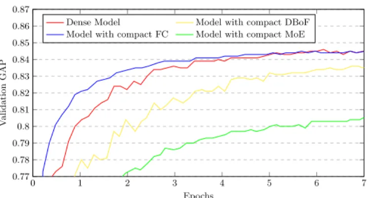
This series of experiments aims at understanding the effect on compactness over different layers. Table 2 shows the result in terms of number of weights, size of the model (MB) and GAP. We also compute the compression ratio with respect to the dense model. The compact fully connected layer achieves a compression rate of 9.5 while having a very similar performance, whereas the compact DBoF and MoE achieve a higher compression rate at the expense of accuracy. Figure 3 shows that the model with a compact FC converges faster than the dense model. The model with a compact DBoF shows a big variance over the validation GAP which can be associated with a difficulty to train. The model with a compact MoE is more stable but at the expense of its performance. Another
0 1 2 3 4 5 6 0.82 0.83 0.84 0.85 0.86 0.87 0.88 Epochs V alidation GAP
Comparison of polling methods used with DBoF embedding
Robust DBoF DBoF w/max pooling DboF w/average pooling
Fig. 2. This graphic shows the impact of robust DBoF (i.e. red line) with n = 10 and k = 15 on the Deep Bag-of-Frames embedding compared to max and average pooling.
series of experiments investigate the effect of adding factors of the compact matrix DC (i.e. the parameters m specified in section 4.3). Table 3 shows that there is no gain in accuracy even if the number of weights increases. It also shows that adding factors has an important effect on the speed of training. On the basis of this result, i.e. given the performance and compression ratio, we can consider that representing the fully connected layer of the base model in a compact fashion can be a good trade-off.
Baseline Model #Weights Size (MB) Compress.
Rate (%) GAP@20 Diff.
Dense Model 45 359 764 173 - 0.846
-Compact DBoF 36 987 540 141 18.4 0.838 -0.008
Compact FC 41 181 844 157 9.2 0.845 -0.001
Compact MoE 12 668 504 48 72.0 0.805 -0.041
Table 2. This table shows the effect of the compactness of different layers. In these experiments, for speeding-up the training phase, we did not use the audio features and exploited only the video information.
#factors #Examples/sec #parameters in FC Layer Compress. Rate of FC layer (%) GAP@20 1 1 052 12 288 99.8 0.861 3 858 73 728 98.8 0.861 6 568 147 456 97.6 0.859 Dense FC 1 007 6 291 456 - 0.861
Table 3. This table shows the evolution of the number of parameters and the accuracy according to the number of factors. Despite the addition of degrees of freedom for the weight matrix of the fully connected layer, the model does not improve in performance. The column #Examples/sec shows the evolution of images per sec processed during the training of the model with a compact FC according to the number of factors.
0 1 2 3 4 5 6 7 0.77 0.78 0.79 0.8 0.81 0.82 0.83 0.84 0.85 0.86 0.87 Epochs V alidation GAP
Comparison of the effect of compactness over different layers with the base model
Dense Model Model with compact DBoF Model with compact FC Model with compact MoE
Fig. 3. Validation GAP according to the number of epochs for different compact models.
5.4 Comparison with related works
Circulant matrices have been used in neural networks in [6]. They proposed to replace fully con-nected layers by a circulant and diagonal matrices where the circulant matrix is learned by a gradient based optimization algorithm and the diagonal matrix is random with values in {-1, 1}. We compare our more general framework with their approach. Figure 4 shows the validation GAP according to the number of epochs of the base model with a compact fully connected layer implemented with both approach. 0 1 2 3 4 5 6 7 8 9 10 0.79 0.8 0.81 0.82 0.83 0.84 0.85 0.86 0.87 0.88 Epochs V alidation GAP
GAP given the pooling method used with DBoF embedding
Compact FC w/general approach Compact FC w/CD and D ∈ {−1, 1}
Fig. 4. This figure shows the GAP difference between the CD approach proposed in [6] and the more generalized DC approach from section 4.3. Instead of having D ∈ {−1, +1} fixed, the generalized approach allows D to be learned.
5.5 Compact Baseline model with different embeddings
To compare the performance and the compression ratio we can expect, we consider different settings where the compact fully connected layer is used together with different embeddings. Figure 5 and Table 4 shows the performance of the base model with DBoF, NetVLAD and NetFV embeddings with a Dense and Compact fully connected layer. Notice that we can get a bigger compression rate with NetVLAD and NetFV due to the fact that the output of the embedding is in a higher dimensional space which implies a larger weight matrix for the fully connected layer. Although the compression rate is higher, it is at the expense of the accuracy.
0 1 2 3 4 5 6 7 8 9 10 0.81 0.82 0.83 0.84 0.85 0.86 0.87 0.88 Epochs V alidation GAP DBoF Compact Dense 0 1 2 3 4 5 6 7 8 9 10 0.81 0.82 0.83 0.84 0.85 0.86 0.87 0.88 Epochs V alidation GAP NetVLAD Compact Dense 0 1 2 3 4 5 6 7 8 9 10 0.81 0.82 0.83 0.84 0.85 0.86 0.87 0.88 Epochs V alidation GAP NetFV Compact Dense
Fig. 5. The figures above show the validation GAP of compact and Dense fully connected layer with different embeddings according to the number of epochs.
Method #Parameters Size (MB) Compress.
Rate (%) GAP@20 DBoF FC Dense 65 795 732 251 - 0.861 FC Circulant 59 528 852 227 9.56 0.861 NetVLAD FC Dense 86 333 460 330 - 0.864 FC Circulant 50 821 140 194 41.1 0.851 NetFisher FC Dense 122 054 676 466 - 0.860 FC Circulant 51 030 036 195 58.1 0.848
Table 4. This table shows the impact of the compression of the fully connected layer of the model archi-tecture shown in Figure 1 with Audio and Video features vector and different types of embeddings. The variable compression rate is due to the different width of the output of the embedding.
5.6 Leverage the diversity of an Ensemble
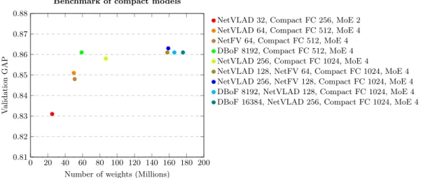
In order to capture the diversity of an Ensemble, we devised a single model architecture combining different embedding layers. As shown in Figure 6, video and audio frames are processed by sev-eral embeddings before being reduced by compact fully connected layers. The results of the fully connected layers are then averaged. The results from the video and audio FC layers are then con-catenated and classified by the MoE and the context Gating layers. Figure 7 shows the result of different models given the number of parameters. All models have compact fully connected layers. Some architectures with diversity manage to improve a little bit better while increasing the number of parameters. Video DBoF NetVLAD NetFV FC FC FC Audio DBoF NetVLAD NetFV FC FC FC average average
concat MoE ContextGating
Embedding Dim Reduction Classification
Fig. 6. This figure shows an evolution of the first architecture from figure 1 with several embeddings. This architecture is made to leverage the diversity of an Ensemble in a single model.
0 20 40 60 80 100 120 140 160 180 200 0.81 0.82 0.83 0.84 0.85 0.86 0.87 0.88
Number of weights (Millions)
V
alidation
GAP
Benchmark of compact models
NetVLAD 32, Compact FC 256, MoE 2 NetVLAD 64, Compact FC 512, MoE 4 NetFV 64, Compact FC 512, MoE 4 DBoF 8192, Compact FC 512, MoE 4 NetVLAD 256, Compact FC 1024, MoE 4
NetVLAD 128, NetFV 64, Compact FC 1024, MoE 4 NetVLAD 256, NetFV 128, Compact FC 1024, MoE 4 DBoF 8192, NetVLAD 128, Compact FC 1024, MoE 4 DBoF 16384, NetVLAD 256, Compact FC 1024, MoE 4
Fig. 7. Benchmark of different models with compact fully connected layers. The figure shows the accuracy according to the number of parameters.
6
Conclusion
In this paper, we demonstrated that circulant matrices can be a great tool to design compact neural network architectures for video classification tasks. We proposed a more general framework which improves the state of the art and conducted a series of experiments aiming at understanding the effect of compactness on different layers. We investigated a model with multiple embeddings to leverage the performance of an Ensemble but found it ineffective. The good performance of Ensemble models, i.e. why aggregating different distinct models performs better that incorporating all the diversity in a single architecture is still an open problem. Our future work will be devoted to address this challenging question and to pursue our effort to devise compact models achieving the same accuracy as larger one, and to study their theoretical properties.
7
Acknowledgement
This work was granted access to the OpenPOWER prototype from GENCI-IDRIS under the Preparatory Access AP010610510 made by GENCI. We would like to thank the staff of IDRIS who was really available for the duration of this work, Abdelmalek Lamine and Tahar Nguira, interns at Wavestone for their work on circulant matrices. Finally, we would also like to thank Wavestone to support this research.
References
1. Abadi, M., Agarwal, A., Barham, P., Brevdo, E., Chen, Z., Citro, C., Corrado, G.S., Davis, A., Dean, J., Devin, M., Ghemawat, S., Goodfellow, I., Harp, A., Irving, G., Isard, M., Jia, Y., Jozefowicz, R., Kaiser, L., Kudlur, M., Levenberg, J., Man´e, D., Monga, R., Moore, S., Murray, D., Olah, C., Schuster, M., Shlens, J., Steiner, B., Sutskever, I., Talwar, K., Tucker, P., Vanhoucke, V., Vasudevan, V., Vi´egas, F., Vinyals, O., Warden, P., Wattenberg, M., Wicke, M., Yu, Y., Zheng, X.: TensorFlow: Large-scale machine learning on heterogeneous systems (2015), https://www.tensorflow.org/, software available from tensorflow.org
2. Abu-El-Haija, S., Kothari, N., Lee, J., Natsev, A.P., Toderici, G., Varadarajan, B., Vijaya-narasimhan, S.: Youtube-8m: A large-scale video classification benchmark. In: arXiv:1609.08675 (2016), https://arxiv.org/pdf/1609.08675v1.pdf
3. Arandjelovi´c, R., Gronat, P., Torii, A., Pajdla, T., Sivic, J.: NetVLAD: CNN architecture for weakly supervised place recognition. In: IEEE Conference on Computer Vision and Pattern Recognition (2016) 4. Arandjelovi´c, R., Gronat, P., Torii, A., Pajdla, T., Sivic, J.: Netvlad: Cnn architecture for weakly supervised place recognition. IEEE Transactions on Pattern Analysis and Machine Intelligence 40(6), 1437–1451 (June 2018). https://doi.org/10.1109/TPAMI.2017.2711011
5. Buciluˇa, C., Caruana, R., Niculescu-Mizil, A.: Model compression. In: Proceedings of the 12th ACM SIGKDD international conference on Knowledge discovery and data mining. pp. 535–541. ACM (2006) 6. Cheng, Y., Yu, F.X., Feris, R.S., Kumar, S., Choudhary, A., Chang, S.F.: An exploration of parameter redundancy in deep networks with circulant projections. In: 2015 IEEE International Conference on Computer Vision (ICCV). pp. 2857–2865 (Dec 2015)
7. Courbariaux, M., Bengio, Y.: Binarynet: Training deep neural networks with weights and activations constrained to +1 or -1. CoRR abs/1602.02830 (2016)
8. Courbariaux, M., Bengio, Y., David, J.P.: Binaryconnect: Training deep neural networks with binary weights during propagations. In: Proceedings of the 28th International Conference on Neural Informa-tion Processing Systems - Volume 2. pp. 3123–3131. NIPS’15, MIT Press, Cambridge, MA, USA (2015), http://dl.acm.org/citation.cfm?id=2969442.2969588
9. Dai, B., Zhu, C., Guo, B., Wipf, D.: Compressing neural networks using the variational information bottleneck. In: Dy, J., Krause, A. (eds.) Proceedings of the 35th International Conference on Ma-chine Learning. Proceedings of MaMa-chine Learning Research, vol. 80, pp. 1143–1152. PMLR, Stock-holmsm¨assan, Stockholm Sweden (10–15 Jul 2018), http://proceedings.mlr.press/v80/dai18d.html 10. Dean, J., Patterson, D., Young, C.: A new golden age in computer architecture:
Empowering the machine-learning revolution. IEEE Micro 38(2), 21–29 (Mar 2018). https://doi.org/10.1109/MM.2018.112130030
11. Denil, M., Shakibi, B., Dinh, L., Ranzato, M.A., de Freitas, N.: Predicting parameters in deep learning. In: Burges, C.J.C., Bottou, L., Welling, M., Ghahramani, Z., Weinberger, K.Q. (eds.) Ad-vances in Neural Information Processing Systems 26, pp. 2148–2156. Curran Associates, Inc. (2013), http://papers.nips.cc/paper/5025-predicting-parameters-in-deep-learning.pdf
12. Gupta, S., Agrawal, A., Gopalakrishnan, K., Narayanan, P.: Deep learning with limited nu-merical precision. In: Proceedings of the 32Nd International Conference on International Con-ference on Machine Learning - Volume 37. pp. 1737–1746. ICML’15, JMLR.org (2015), http://dl.acm.org/citation.cfm?id=3045118.3045303
13. Han, S., Mao, H., Dally, W.J.: Deep compression: Compressing deep neural networks with pruning, trained quantization and huffman coding. International Conference on Learning Representations (ICLR) (2016)
14. Hinrichs, A., Vyb´ıral, J.: Johnson-lindenstrauss lemma for circulant matrices. Random Structures & Algorithms 39(3), 391–398 (2011)
15. Hinton, G., Vinyals, O., Dean, J.: Distilling the knowledge in a neural network. In: NIPS Deep Learning and Representation Learning Workshop (2015), http://arxiv.org/abs/1503.02531
16. Jaderberg, M., Vedaldi, A., Zisserman, A.: Speeding up convolutional neural networks with low rank expansions. CoRR abs/1405.3866 (2014)
17. J´egou, H., Douze, M., Schmid, C., P´erez, P.: Aggregating local descriptors into a compact im-age representation. In: CVPR 2010 - 23rd IEEE Conference on Computer Vision & Pattern Recognition. pp. 3304–3311. IEEE Computer Society, San Francisco, United States (Jun 2010). https://doi.org/10.1109/CVPR.2010.5540039, https://hal.inria.fr/inria-00548637
18. Jiang, Y.G., Wu, Z., Wang, J., Xue, X., Chang, S.F.: Exploiting feature and class relationships in video categorization with regularized deep neural networks. IEEE Transactions on Pattern Anal-ysis and Machine Intelligence 40(2), 352–364 (2018). https://doi.org/10.1109/TPAMI.2017.2670560, https://doi.org/10.1109/TPAMI.2017.2670560
19. Jordan, M.I., Jacobs, R.A.: Hierarchical mixtures of experts and the em algorithm. In: Proceedings of 1993 International Conference on Neural Networks (IJCNN-93-Nagoya, Japan). vol. 2, pp. 1339–1344 vol.2 (Oct 1993). https://doi.org/10.1109/IJCNN.1993.716791
20. Karpathy, A., Toderici, G., Shetty, S., Leung, T., Sukthankar, R., Fei-Fei, L.: Large-scale video classi-fication with convolutional neural networks. In: CVPR (2014)
21. Karpathy, A., Toderici, G., Shetty, S., Leung, T., Sukthankar, R., Fei-Fei, L.: Large-scale video classifi-cation with convolutional neural networks. In: Proceedings of the IEEE conference on Computer Vision and Pattern Recognition. pp. 1725–1732 (2014)
22. Li, F., Gan, C., Liu, X., Bian, Y., Long, X., Li, Y., Li, Z., Zhou, J., Wen, S.: Temporal modeling approaches for large-scale youtube-8m video understanding. CoRR abs/1707.04555 (2017)
23. Lin, J., Rao, Y., Lu, J., Zhou, J.: Runtime neural pruning. In: Guyon, I., Luxburg, U.V., Bengio, S., Wal-lach, H., Fergus, R., Vishwanathan, S., Garnett, R. (eds.) Advances in Neural Information Processing Systems 30, pp. 2181–2191. Curran Associates, Inc. (2017), http://papers.nips.cc/paper/6813-runtime-neural-pruning.pdf
24. Mellempudi, N., Kundu, A., Mudigere, D., Das, D., Kaul, B., Dubey, P.: Ternary neural networks with fine-grained quantization. CoRR abs/1705.01462 (2017)
25. Miech, A., Laptev, I., Sivic, J.: Learnable pooling with context gating for video classification. CoRR abs/1706.06905 (2017)
26. M¨uller-Quade, J., Aagedal, H., Beth, T., Schmid, M.: Algorithmic design of diffractive optical systems for information processing. Physica D: Nonlinear Phenomena 120(1-2), 196–205 (1998)
27. Perronnin, F., Dance, C.: Fisher kernels on visual vocabularies for image categorization. In: 2007 IEEE Conference on Computer Vision and Pattern Recognition. pp. 1–8 (June 2007). https://doi.org/10.1109/CVPR.2007.383266
28. Rastegari, M., Ordonez, V., Redmon, J., Farhadi, A.: Xnor-net: Imagenet classification using binary convolutional neural networks. In: ECCV (2016)
29. S´anchez, J., Perronnin, F., Mensink, T., Verbeek, J.: Image classification with the fisher vector: Theory and practice. Int. J. Comput. Vision 105(3), 222–245 (Dec 2013). https://doi.org/10.1007/s11263-013-0636-x, http://dx.doi.org/10.1007/s11263-013-0636-x
30. Schmid, M., Steinwandt, R., M¨uller-Quade, J., R¨otteler, M., Beth, T.: Decomposing a matrix into circulant and diagonal factors. Linear Algebra and its Applications 306(1-3), 131–143 (2000)
31. Sindhwani, V., Sainath, T., Kumar, S.: Structured transforms for small-footprint deep learn-ing. In: Cortes, C., Lawrence, N.D., Lee, D.D., Sugiyama, M., Garnett, R. (eds.) Advances in Neural Information Processing Systems 28, pp. 3088–3096. Curran Associates, Inc. (2015), http://papers.nips.cc/paper/5869-structured-transforms-for-small-footprint-deep-learning.pdf
32. Skalic, M., Pekalski, M., Pan, X.E.: Deep learning methods for efficient large scale video labeling. arXiv preprint arXiv:1706.04572 (2017)
33. Vyb´ıral, J.: A variant of the johnson–lindenstrauss lemma for circulant matrices. Journal of Func-tional Analysis 260(4), 1096 – 1105 (2011). https://doi.org/https://doi.org/10.1016/j.jfa.2010.11.014, http://www.sciencedirect.com/science/article/pii/S0022123610004507
34. Wang, H., Zhang, T., Wu, J.: The monkeytyping solution to the youtube-8m video understanding challenge. CoRR abs/1706.05150 (2017)
35. Yang, Z., Moczulski, M., Denil, M., d. Freitas, N., Smola, A., Song, L., Wang, Z.: Deep fried con-vnets. In: 2015 IEEE International Conference on Computer Vision (ICCV). pp. 1476–1483 (Dec 2015). https://doi.org/10.1109/ICCV.2015.173
36. Yu, X., Liu, T., Wang, X., Tao, D.: On compressing deep models by low rank and sparse decomposition. In: 2017 IEEE Conference on Computer Vision and Pattern Recognition (CVPR). pp. 67–76 (July 2017). https://doi.org/10.1109/CVPR.2017.15
37. Yue-Hei Ng, J., Hausknecht, M., Vijayanarasimhan, S., Vinyals, O., Monga, R., Toderici, G.: Beyond short snippets: Deep networks for video classification. In: Proceedings of the IEEE conference on com-puter vision and pattern recognition. pp. 4694–4702 (2015)